The Effects of Sample Size on the Estimation of Regression Mixture Models
Thomas Jaki
1Minjung Kim
2Andrea Lamont
3Melissa George
4Chi Chang
5Daniel Feaster
6M. Lee Van Horn
7This research was supported by grant number R01HD054736, M. Lee Van Horn (PI), funded by
the National Institute of Child Health and Human Development and grant MR/L010658/1 from
the Medical Research Council of the United Kingdom, Thomas Jaki (PI). Questions or comments
should be addressed to the senior and corresponding author, M. Lee Van Horn, [email protected].
1 Department of Mathematics and Statistics, Lancaster University, UK
2 Department of Educational Studies, Ohio State University
3 Department of Psychology, University of South Carolina, Columbia
4 Department of Human Development & Family Studies, Colorado State University
5 College of Human Medicine, Michigan State University
6 Department of Public Health Sciences, Division of Biostatistics, University of Miami
Abstract
Regression mixture models are a statistical approach used for estimating heterogeneity in effects.
This study investigates the impact of sample size on regression mixture’s ability to produce
‘stable’ results. Monte Carlo simulations and analysis of resamples from an application dataset
were used to illustrate the types of problems that may occur with small samples in real datasets.
The results
suggest: 1) when class separation is low very large sample sizes may be needed to
obtain stable results; 2) it may often be necessary to consider a preponderance of evidence in
latent class enumeration; 3) regression mixtures with ordinal outcomes result in even more
instability; and 4) with small samples it is possible to obtain spurious results without any clear
indication of there being a problem. indicate a substantial impact of small samples (relative to
class separation) on both the number of classes supported by the data and estimates of
differential effects in those classes. In some cases, there was no indication of invalid results, and
yet the reported effects were opposite to those that existed in reality. This concerning finding was
related to another: that dramatic differences sometimes appeared between multiple subsamples
from the same data as sample size decreased. Overall these results suggest that sample sizes
much larger than those typically considered large are needed to assure stable results (500 to 1000
subjects were needed for most analyses in this paper). Great caution is therefore urged in the use
of regression mixtures with small samples, and the results highlight the importance of model
validation. Because no one simulation can provide comprehensive guidelines for required sample
sizes, however, it is recommended that multiple simulations reflecting the structure of the dataset
of interest be conducted to understand model stability for a given result.
The Effects of Sample Size on the Estimation of Regression Mixture Models
The notion that individuals vary in their response to their environment has been
well-accepted across substantive fields. Leading theories in the behavioral, social, and health sciences
emphasize the synergistic role of environmental risk in individual development (Bronfenbrenner,
2005; Elder, 1998; Patterson, DeBaryshe, & Ramsey, 1989; Sampson & Laub, 1993) and
consequently the search for differential effects – i.e., individual differences in the relationship
between a predictor and an outcome – has become of increased salience to applied researchers.
Traditional approaches for assessing differential effects involve the inclusion of a multiplicative
interaction term into a regression equation. This method is intuitive and useful for testing
differential effects which have been hypothesized a priori and involve observed subgroups. An
alternative strategy, regression mixture modeling, utilizes a finite mixture model framework to
capture unobserved heterogeneity in the effects of predictors on outcomes (Desarbo, Jedidi, &
Sinha, 2001). In other words, regression mixture models are an exploratory approach to finding
differential effects that do not require their predictors to be measured (Dyer, Pleck, & McBride,
2012; Van Horn et al., 2009).
This paper uses simulations and resamples from applied data to show how sample size
impacts regression mixture results with the aim of providing users of this method with a starting
point for selecting their samples. As regression mixture modeling is a relatively new method,
further work is needed to understand the conditions under which models will provide unbiased
and stable estimates of differential effects. The question of what sample size is needed to achieve
requirements
depend
s
critically on class separation, with
both
regression-parameter estimation
and latent-class enumeration being a function of both sample size and class separation.
We
therefore hypothesize that, as sample size and/or class separation decrease the likelihood of
unstable solutions will increase.
Methodological Overview
Regression mixture models are a specific form of finite mixture model. The latter term
refers to a broad class of statistical models that estimate population heterogeneity through a finite
set of empirically derived latent classes. Regression mixture models typically aim to identify
discrete differences in the effect of a predictor on an outcome. This differs from other more
commonly known mixture approaches, such as growth mixture models (B. Muthen, 2006; B.
Muthén, Collins, & Sayer, 2001; B. O. Muthen et al., 2002) and semi-parametric models (D. S.
Nagin, 2005; Daniel S. Nagin, Farrington, & Moffitt, 1995), in that the latent classes in a
regression mixture are defined by bewteen-class differences in the associations between two
variables, rather than between-class differences in the means or variances of a single variable
(Desarbo et al., 2001; Van Horn et al., 2009; Wedel & Desarbo, 1994).
The formulation,
estimation, and details around the specification of regression mixtures are already well
established
(M. L. Van Horn et al., 2015)
. This paper focuses on helping users of regression
mixtures understand the role that sample size and class seperation plays in the stability of
regression mixture results.
Sample size in mixture models
parameters?
(It should be noted here that, if the hypothesis concerns latent-class enumeration, there is typically no alpha level associated with the test).
This is a question of obtaining the sampling distribution for a specific parameter,
and it can in principle be derived analytically. However, mixture models include many
parameters that impact power, and attempts at latent-class enumeration typically rely on
comparison of penalized information criteria, such as the Bayesian Information Criterion (BIC),
for which there is no known sampling distribution. Thus, power for regression mixtures is
typically estimated using Monte Carlo simulation.
This paper raises a The
second
perspective relates to the present paper’s hypothesis that that a second issue exists withrelated to
finite
mixture
s
in general, and
with
regression mixtures in particular. Because mixture models (Bauer &
Curran, 2003, 2004) and especially regression mixtures (George et al., 2011; Van Horn et al.,
2012) rely on strong distributional assumptions for parameter estimation, we
hypothesize aim to show
that
model results
will
be increasingly unstable with smaller samples to the point that – even under ideal
conditions – such models will yield more extreme results than expected – i.e. results
may be
far outside
of the confidence interval suggested by estimated standard errors.
Rather, this paper uses both simulations of selected scenarios and resampling of a real dataset to
raise researchers’ awareness of the types of problems that regression mixture modeling is likely
to encounter when small samples are use
d, we focus specifically on the interplay between class
separation and sample size while also looking at the proportion of subjects in each class.d.
Much work has looked at latent class enumeration, with some also looking at parameter
estimation, with mixture models in general. Of particular note is work which has looked at
differential effects, intercept differences may be small to nonexistent. It should also be noted that
Sarstedt and Schwaiger (2008) did not evaluate the precision or stability of parameter estimates.
One other study examined sample size requirements for regression mixtures, this time
using a negative binomial model. Park, Lord, and Hart (2010) incorporated design features
typically seen in highway crash data into their simulation, examining bias in parameter estimates,
and found large bias in the dispersion parameter in samples less than n=2,000 under realistic
conditions. They noted unstable solutions with small sample sizes and moderate or low effects,
but also found that under conditions of high class separation (i.e., large mean differences
between classes), their model was stable for samples as small as n=300. A reason for these
discrepant results has to do with how much classes differ; as Park, Lord, and Hart (2010) put it,
“the sample size need not be large for well-separated data, but it can be huge for a
poorly-separated case.” Class separation is at its lowest when differences between latent classes are
solely a function of differences in regression weights with no mean differences; and in this case,
the multivariate distributions of the data for the different classes overlap almost completely. This
is also the point at which regression mixtures fulfill their promise as a method for exploring for
differential effects, since they should be capable of finding discrete groups of respondents
distinguished primarily by differences in regression weights.
The Current Study
power, but rather parameter estimates which do not represent the population well. Based on the
results of previous applied research and simulations, we hypothesize that the use of small
samples in regression mixture models will increase the likelihood of extreme results, such that
estimates of regression parameters across classes will be biased away from each other, while the
confidence intervals of the estimates will be too narrow.
We also hypothesize that class
enumeration will become more difficult with small samples, and that there will be an increasing
number of convergence problems for the model.Additional analyses focus on the role of class
separation in this relationship.
Ordinal logistic regression mixture models have been found effective for evaluating
differential effects in the presence of skewed outcomes (Fagan, Van Horn, Hawkins, & Jaki,
2012; George, Yang, Van Horn, et al., 2013; Van Horn et al., 2012). Therefore, we
will
also test
the hypothesis that the effects of sample size will be stronger on the ordinal logistic model
than
on other models because they require additional parameters, and
because less information is
available for analyses with ordinal outcomes.
Methods: Simulation Study
Five Hundred The
Monte Carlo simulation
s
phase of our study included 500
relatively simple context.
The initial simulations used one predictor, X, and one outcome
variable, Y. The regression relationship for class 1 was Y = 0.70X + e, and for class 2, Y =
0.20X + e.
In both classes, tT
he predictor and the residuals, e, were drawn from a
standard
normal distribution with the residuals for Y scaled so that the standard deviation of Y is one.
Thus, the slope of the predictor is equal to the correlation of X and Y.
To answer our research questions, we examined 18Eighteen simulation
conditions
were
examined
. For the first 10 conditions, the total number of individuals in the data set
(6,000,
3,000, 1,000, 500, and 200)
as well as the proportion of the sample in each class
(50% in each
class and 75% in class 1 and 25% in class 2) was
varied
across conditions
.
Our five chosen levels
of overall sample size were 6,000, 3,000, 1,000, 500, and 200.
The largest case, 6,000
individuals in total was chosen based on prior studies (e.g., Van Horn et al., 2009; Van Horn et
al., 2012) that suggested this was a sufficient number of individuals to find expected results.
The
smallest total sample size examined was 200 cases. For each sample size, two different balance
designs for latent classes were examined: i.e., 50/50 and 75/25 splits of individuals in class 1 and
class 2, respectively.
mixture model, as these results differed across criteria. The percentage of
times for which
the two-class
model would have been selected over the one-class or the three-class model were reported to
better understand failures to select the true two-class model, we also calculated the percentage of
times the three-class model is chosen over the two-class model; but importantly, we considered
failure of the three-class model to converge as indicating support for the two-class result. This
decision was based on our previous experience that over-parameterized models frequently fail to
converge to a replicated loglikelihood (LL) value. This assumption changed results dramatically
only for the ordinal outcomes model, class enumeration tables without this assumption are
available from the authors upon request. Finally, the average size of the smallest class across
simulations was recorded for each condition; and when the smallest class is relatively small (e.g.,
lower than 10% of the overall sample size), it was necessary to give further consideration to
whether there was sufficient evidence to support a meaningful additional class, or if the apparent
presence of an additional class was due to outliers or violations of the distributional assumption.
We note that 10% is an arbitrary number and that it is possible to have true and meaningful
classes below this size, given enough information in the data to reliably detect these classes.
All study simulation conditions were evaluated for replicated convergence, model fit,
class enumeration and parameter estimation. Replicated-convergence is defined as a simulation
run in which 1) a solution was obtained and 2) the log-likelihood value was replicated to the next
integer in at least two of the 24 starting values.
for which the true parameter is contained in the 95% confidence interval. Lastly, we displayed
the distribution of slopes across simulations for conditions with smaller sample sizes. This serves
two purposes. First, it helps to identify the presence of outliers in the estimated slopes; and,
secondly, it helps to assess the robustness of the estimation and underlying sampling distribution.
To correct for the problem of label-switching in simulations, classes were sorted such that the
class with the stronger effect of X on Y was always class 1 (McLachlan & Peel, 2000; Sperrin,
Jaki, & Wit, 2010). In cases where the two classes were not distinct, as evidenced by the
distribution of the parameter estimates, average parameter estimates were somewhat biased in
favor of the correct solution because of this class sorting.
Results: Simulation Study
problem was largely due to model misspecification, i.e., resulted from estimating a
n incorrect
three-class model
when there were in fact two classes in the population
.
in the population - they do suggest that its performance when classifying individuals will be
poor.
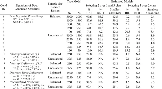
Our class-enumeration results are provided in Table 2. For the basic set-up, the BIC
criterion usually yielded the correct two-class solution when sample sizes were 3,000 or more
(conditions 1, 2, 6, and 7), but none of the criteria performed well when sample sizes were
smaller than that. These analyses also looked at the size of the smallest class for both the two-
and class solutions, and found that the average class size of the smallest class for the
three-class solution was always well below 10% of the overall sample size, whereas in all two-three-class
solutions it was over 10%. In practice
, it appears that small classes can be an indicator of a
spurious class. For these simulations, if an arbitrary criterion of 10% in the smallest class was
utilized to exclude a result,
the three-class solution would usually be excluded from
consideration
because of the size of the smallest class. ; a two-class solution would likely be
chosen over a one-class solution in cases where the smallest class was moderately large and the
other criteria for the one-class and two-class solutions were similar.
On the whole, these
simulations suggest that
for
samples of 1,000 or more
individuals researchers
are reasonably
likely to arrive at the correct two-class solution for this data generating scenario
, while smaller
samples are not if all information is used rather than any one criterion
.
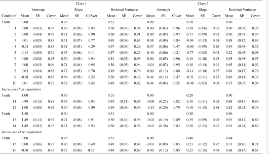
As shown in Table 3, average model parameters were reasonably well estimated for all
conditions in class 1 (with the larger regression weight). However, in class 2, bias in all
parameters increased as sample size or class separation decreased, with class means (intercepts)
showing an upward bias, and regression weights and variances showing a downward bias. While
some of the model-parameter estimates appeared reasonable even with small samples, the
coverage probabilities for the parameter estimates –defined as the percentage of simulations for
which the true value is inside the 95% confidence interval – revealed serious problems with
estimated confidence intervals as sample size decreased. Note that even in conditions with
sample sizes over 1000, coverage was slightly less than desirable for the slope parameters. This
suggests that estimated standard errors were too small. The very poor coverage estimates
observed for sample sizes of 200 and 500 - especially for class 2 - could be a function of model
instability as some simulations yielded extreme estimates (
It should be nN
ote
d here
that, for the
residual variances, the 95% confidence interval was not accurate
,
because variances do not
follow a t distribution).
We further investigated model instability by examining the distribution of regression
weights across simulations. Figure 1 presents histograms of the slopes for both classes mixed, for
the conditions with less than 3,000 observations. The conditions with 3,000 and 6,000
regression weights in each class. These peaks were evident in conditions 3 and 8, although both
conditions feature some extreme outliers. However, at sample sizes of 500 and 200, the two
peaks merge into one and there are many outliers, both above and below the true values.
As sample sizes decrease, we also expect wider confidence intervals and more variation
across simulations. However, the extreme results seen in some simulations are not just a function
of sampling variability, as the models’ estimated standard errors are still relatively low and some
of the parameter estimates are more than 15 standard errors from the true value. We then
examined individual results from the small samples that showed extreme values, and found that
many of the simulation results with extreme regression weights contained quite small classes that
in practice would probably not be considered strong evidence for differential effects. However, it
was also not uncommon to find results that featured: 1) strong effects in the opposite direction to
the true effects with reasonably large class sizes, 2) replicated LL values, and 3) no other
evidence that the result was erroneous. Small samples, in other words, could make it extremely
difficult to discover that there is a problem with a given finding.
[Figure 1]
simulations that correctly identified two latent classes
crashing
from 87.9% to just 4.2%. Finally, in
conditions 17 and
18, (not included in Table 3 because of the additional parameters) we
examined the impact of including more information in the regression mixture model by adding
an additional predictor. In this condition with a sample size of 500, the BIC found the correct
two class solution in more than 97% of the simulations. Parameter estimates from these models
were all reasonable, although coverage rates were somewhat less than .95 for the models with
strong class separation and far less than .95 for models with weaker class separation.
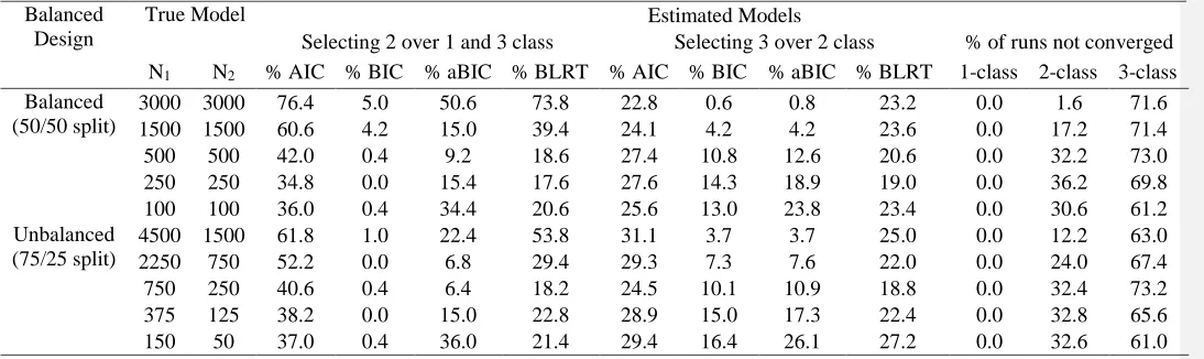
We also investigated the use of an ordinal logistic model for identifying the correct
number of classes (Table 4), which was recommended by Van Horn et al. (2012) and George et
al. (2013) as a method for addressing non-normal errors. As in the normally distributed model,
there were substantial issues with model convergence for the two-class ordinal logistic models
when the sample size fell below 3,000. Further, even with 6,000 observations (the same number
as in George et al., 2013), the BIC chose the correct two-class model in only 5% of the
simulation replications. The main difference between this result and the previously reported
results (George et al, 2013; Van Horn et al., 2012) is that
ours hadhere there was
no intercept
difference
s
. When we added a between-classes intercept difference of .5 standard deviations, we
replicated the previous results, choosing the correct two-class solution in 95% of the simulations.
With large sample sizes, the BLRT and aBIC had better, though still inadequate results; in the
best case scenario with a sample of 3,000 the BLRT found two classes in 74% of simulations.
Because the correct number of classes was rarely selected, parameter estimates are not reported.
[Table 4]
Our initial simulations examined the effects of sample size on regression mixture models
when the only feature defining latent classes was the heterogeneous effects of a predictor on an
outcome. We deliberately
choose chose
a simulation scenario that was ideal in terms of
distributional assumptions and the number of latent classes, but rendered more difficult by the
very weak class separation caused by the lack of mean differences between classes in the
outcome and no other predictors with which to separate the latent classes. We showed that, in
such circumstances, entropy in the true model is very low and that model convergence to a
replicated LL value becomes increasingly unlikely as sample sizes drop to 1,000 or less. None of
the model-selection criteria were effective in selecting the true model when samples were less
than 3000 although
when a preponderance of evidence was used the correct solution could be
found , and their performance was merely adequate
with samples of 1,000. The problem appears
to be not only a lack of power, but also the selection of solutions with superfluous, typically very
small, classes.
The problem is reduced if solutions with small classes are eliminated from
consideration, this leaves open the question of how to find true small classes. We suspect that in
this case either substantial class separation or very large sample sizes will be needed.
We found
that, with ordinal logistic regression model
, all the selection criteria were underpowered; and that
and no intercept differences
it was possible to arrive at the right number of classes
, but
only if a
preponderance of the evidence was used – an approach that implies never choosing solutions
with any classes that contain 10% or less of the respondents.
When there are no intercept
differences between classes, it is quite difficult to arrive at the correct number of classes using
the ordinal logistic regression mixtures.We note that a limitation of this study is that we only
classes without increasing class separation would increase required sample size because of the
need to estimate more parameters without having much additional information.
When the correct number of latent classes were found, model-parameter estimates were
on average reasonable, except for
the very small
class sizes of 500 and below. However, this
hide
s
an additional issue. With sample sizes this small, there were many cases in which multiple
classes were supported and apparently reasonable solutions found, but where the parameter
estimates were extreme, or even opposite of the true values.
In short, aA
lthough regression
mixture models work well with large samples, using such models with small samples appears to
be a dangerous proposition
, as it will never be completely clear that the results are correct, or
even how to identify that they are suspect
.
To better understand these results we further investigated the effects of class separation
on required sample size, showing that increasing class separation led to adequate results with
samples of 500 and decreasing class separation resulted in samples of 1000 being inadequate to
find differential effects (the correct number of classes). A promising result came from including
additional predictors in the model, in this case model performance improved dramatically.
This
final result calls for more research as we examined only two conditions. Finally, we examined
the implications of these results when using ordinal outcomes, finding that this case requires
additional class separation if the correct number of classes is to be found.
Applied Example: Introduction
one defined by low achievement (especially in reading but also in mathematics outcomes); one
defined by a strong effect of basic needs (e.g., housing, food, and clothing); and the last being
resilient to the effects of a lack of basic needs. Because the latter two classes had similar means
for achievement, the class separation between them was weak. Nevertheless, the three classes
appeared to be robust, especially with regards to the inclusion of covariates, and the study had a
reasonably large
sample size of 6,305. This data provides us with an opportunity for assessing
what would have happened if a smaller dataset had been used
with applied rather than simulated
data..
Applied Example: Methods
Analyses were run on the full dataset that includes 6,305 students. To assess the effects of
running regression mixtures on small samples we drew 500 replications without replacement
from the full dataset of the same four sizes used in the simulation study described above (i.e.,
n=200, 500, 1,000, and 3,000). For each sample-size condition, analyses were run for all 500
datasets to evaluate the effect of sample size on class enumeration and parameter estimates,
using the same methods as in our simulations. Given that the true population values for the
empirical data were not known, we assessed the differences in the model results between the full
dataset with 6,305 cases and the subsets of the data with smaller sample sizes. We were
especially interested in the between-subsample differences within each condition, as these would
indicate the range of results that might arise across many small samples.
Applied Example: Results
The first step in this phase of our analyses was to examine the regression mixture solution
for the full sample. The BIC chose a two-class solution in the full sample, the aBIC was more
equivocal: with the two and three-class solutions being about the same, but the latter’s third class
was small, with 8% of the students. We chose to retain the two-class solution.
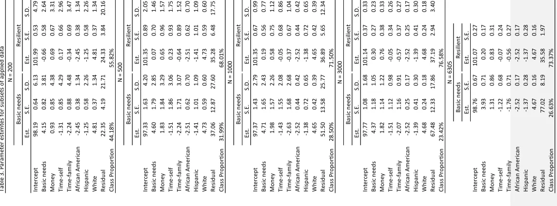
Its The
classes
were similar in substance to those already published; the first class containing 27% of the
students, and defined by a strong positive effect of basic needs (B = 3.93, SE =.71) and a weaker
negative effect of time spent with family (B = -1.76, SE = .71), and the second class with 73% of
the students, featuring a weak positive effect of money (B = .83, SE = .31) and a weak negative
effect of time spent with family (B = -.56, SE = .27). The intercepts for the two classes were
quite similar
, B = 98.74, SE = .67 in class one and B = 101.07, SE = .27 in Class 2
.
two-class model in about 30% of the simulations with sample sizes of 200, and convergence was a
problem in most simulations for the three-class model.
With the applied data, however,
convergence was rarely a problem with a sample of 200, the two-class model converged 96% of
the time, and the three-class model converged 94% of the time
, and convergence was even
higher in larger samples
. This is consistent with previous results in which convergence became a
problem when models were over-parameterized with simulated data that was perfectly behaved
(M. Lee Van Horn et al., 2015), but convergence is generally not a problem with applied data,
which never perfectly meets
researchers’
model assumptions. While convergence was not a
problem with the applied data, replicating the two-class solution was much more difficult. With a
sample size of 3,000, only 141 of the 500 replications
choose chose
the two-class over the
one-class and three-one-class models using the BIC. This fell to 73 out of 500 replications when the
sample size was reduced to 1,000, but then went back up again to 154 out of 500 replications
when the sample fell further, to 500; and edged up again, to 181 out of 500 replications, with the
very lowest sample size, 200. By this criterion alone, then, it appeared that a sample size of 200
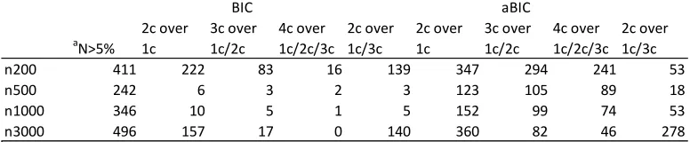
yielded the best model performance. We further explored these results by taking the size of the
smallest class into account. When classes that contained less than 5% of the students were
excluded from consideration, the two-class model was chosen 140 times with a sample of 3,000,
less than five times when the sample was 1,000 or 500, and 139 times when it was 200.
Using
the aBIC increased all these numbers somewhat: with the two-class model being chosen 280,
Finally, we examined parameter estimates across replications within each condition.
Here, we focused on the regression weight for the effects of students’ basic needs, looking only
at those cases where the smallest class contained over 5% of the sample, since cases with smaller
classes than that typically had extreme outliers. In other words, we assumed that the analyst
would have arrived at the two-class model even if the model-selection criteria did not clearly
indicated support for two classes. The number of 500 simulations for which the smallest class in
the two-class solution contained more than 5% of the students was 411 when the sample size was
200, 242 when it was 500, 346 when it was 1,000, and 496 when it was 3,000. Figure 2 presents
histograms
of each condition
of regression weights for the effects of basic needs
for each
condition
, and the full model results are included in Appendix A. Classes are not sorted here
(since it would clearly be problematic in the small-sample conditions),
and thus
if the solution
from is stable and matches
the full dataset
is stable
– we should see two relatively normal
distributions, with one centered on about 0.2 (the non-significant effect of basic needs in the
resilient class) and the other centered on about 3.9. When the sample size was 3,000, the results
were almost perfectmirrored this,
with nearly complete separation between the different classes.
Thus, any 2-class solution with a sample of 3000 would lead to similar results Neither the BIC
larger than would be suggested by
the
estimated standard error
; and in fact, the standard
deviation of the slopes for the largest class across all replications was 2.1, substantially larger
than the standard error that it supposedly represents
. Finally, the model results mostly break
down with samples of 500 and 200, which provided vague, general evidence for the existence of
the class with no basic-need effects, but rarely replicated the results from the full sample.
Applied Example: Conclusions
Examining small sample sizes by resampling a previously published example dataset
yielded some interesting results. First, it cc
onfirmed a previous antidotal finding that
however, using small samples would not only yield quite inaccurate results, but estimated
standard errors that give the researcher a false sense of confidence in such results.
Discussion
One of the most common questions asked at presentations on regression mixture models
concerns the sample size required to use this method.
Our purpose in this study was to help
applied researchers understand the interplay between class separation and sample size when
estimating regression mixture models with continuous and ordinal outcomes. Looking across all
results of this study suggests: 1) when class separation is low (as is typical in regression
mixtures), sample sizes as much as an order of magnitude greater than suggested by previous
research may be needed to obtain stable results; 2) there is a direct relationship between class
separation and required sample size such that increasing class separation would make most
results stable, although potentially at the cost of losing what made a regression mixture useful; 3)
regression mixtures with ordinal outcomes result in even more instability; 4) with small samples
it is possible to obtain spurious results without any clear indication of there being a problem; 5)
very small latent classes may be an indicator of a spurious result (it isn’t clear to us how truly
small classes can be reliably identified when class separation is low); 6) higher values of entropy
are not necessarily indicative of a correct model; and 7) at least within the range of a 25% to
75% split between classes, the effects of class size were less in our study than of sample size.
This study provides insight into that question. We specifically focused on cases with very
weak class separation, because it is in such cases that regression mixture models are truly defined
by differential effects. If there are large differences in the means of the outcomes between
This study found that when there were no mean differences between classes, even when data was
generated to be ideal (in the sense that distributional assumptions were met in every class),
sample size had a clear effect on both latent-class enumeration and parameter recovery. As
sample size decreased, penalized information criteria and the BLRT frequently failed to find the
true number of classes; and, when the true number of classes was found, these models struggled
to distinguish the true differences in parameters between classes. Classes with less residual error
were generally better estimated.
We conducted a series of additional simulations designed to make the point that sample
size requirements are a function of sample size, class separation, and available information. With
increased class separation, smaller samples will still lead to replicable results. With decreased
class separation, even larger samples are needed. And, when more information – such as
additional covariates – is brought into the model, results become more stable. The final point is
interesting because it is often fairly easy for investigators to add additional predictors into a
study.
T
ak
en
as a w
h
o
le, o
u
r resu
lts clearly
d
em
o
n
strate an
im
p
act o
f sam
p
le size o
n
reg
ressio
n
m
ix
tu
re m
o
d
els, w
ith
serio
u
s p
ro
b
lem
s arisin
g
in
sm
all sam
p
les. W
e are relu
ctant to provide specific “rules of thumb” for sample-size requirements, which will differ strongly from study to study, and maintain that using simulations that replicate the specific details of an applicatio
n is the best way to estimate that application’s stability. Ultimately, this paper verifies the hypothesis that regression mixture models are best thought of as a large-sample method (Van Horn et al., 2009) by demonstrating the potential negative impacts of small samples on both enumeration and parameter estimation. Crucially, this study also showed that when samples are relatively small, there is considerable variability between different samples; the estimated standard errors are often downward-biased; and it is possible to obtain results that do not reflect the true characteristics of the studied population (and may even in the wrong direction!), but which include no discernible evidence of such a problem. This is undoubtedly a major limitation of regression mixture modeling, and publication of the results of such modeling using only one small sample appears ill-advised unless class separation is very strong.
Akaike, H. (1973). Information theory and extension of the Maximum Likelihood Principle. In B. N. Petrov& F. Csaki (Eds.), Second International Symposium on Information Theory (pp. 267-281).
Budapest: Springer.
Bauer, D. J., & Curran, P. J. (2003). Distributional assumptions of growth mixture models: Implications
for overextraction of latent trajectory classes. Psychological Methods, 8, 338-363.
Bauer, D. J., & Curran, P. J. (2004). The integration of continuous and discrete latent variable models:
Bozdogan, H. (1994). Mixture-model cluster analysis using model selection criteria and a new
information measure of complexity Proceeding of the first US/Japan conference on frontiers of
statistical modeling”: And information approach (Vol. 2, pp. 69-113). Boston: Kluwer Academic Publishing.
Bronfenbrenner, U. (Ed.). (2005). Making human beings human: Bioecological perspectives on human
development. Thousand Oaks, CA: Sage Publications.
Desarbo, W. S., Jedidi, K., & Sinha, I. (2001). Customer value analysis in a heterogeneous market.
Strategic Management Journal, 22, 845-857.
Dunn, L. M., & Dunn, L. M. (1981). Peabody Picture Vocabulary Test-Revised. Circle Pines, MN: American
Guidance Service.
Dunst, C. J., & Leet, H. E. (1994). Measuring the adequacy of resources in households with young
children. In C. J. Dunst (Ed.), Supporting & strengthening families, Vol (pp. 105-114). Cambridge,
MA: Brookline Books Inc.
Dunst, C. J., Leet, H. E., & Trivette, C. M. (1988). Family resources, personal well-being, and early
intervention. Journal of Special Education, 22(1), 108-116.
Dyer, W. J., Pleck, J., & McBride, B. (2012). Using mixture regression to identify varying effects: A
demonstration with parental incarceration. Journal of Marriage and Family, 74, 1129-1148.
Elder, G. H. (1998). The Life Course Developmental Theory. Child Development, 69(1), 1-12.
Fagan, A. A., Van Horn, M. L., Hawkins, J., & Jaki, T. (2012). Differential effects of parental controls on
adolescent substance use: For whom is the family most important? Quantitative Criminology,
Published online Sept 4.
George, M. R. W., Yang, N., Jaki, T., Feaster, D., Smith, J., & Van Horn, M. L. (2013). Regression mixtures
for modeling differential effects and non-normal distributions. Multivariate Behavioral Research,
George, M. R. W., Yang, N., Van Horn, M. L., Smith, J., Jaki, T., Feaster, D., . . . Howe, G. (2011). Using
regression mixture models with non-normal data: Examining an ordered polytomous approach.
Journal of Statistical Compution and Simulation.
George, M. R. W., Yang, N., Van Horn, M. L., Smith, J., Jaki, T., Feaster, D. J., & Maysn, K. (2012). Using
regression mixture models with non-normal data: Examining an ordered polytomous approach. J
Stat Comput Simul, Published Online Before Print
George, M. R. W., Yang, N., Van Horn, M. L., Smith, J., Jaki, T., Feaster, D. J., & Maysn, K. (2013). Using
regression mixture models with non-normal data: Examining an ordered polytomous approach.
Journal of Statistical Computation and Simulation, 83(4), 757-770.
Kim, M., Vermunt, J., Bakk, Z., Jaki, T., & Van Horn, M. L. (2016). Modeling predictors of latent classes in
regression mixture models. Structural Equation Modeling, 23(601-614).
Liu, M., & Lin, T. I. (2014). A Skew-Normal Mixture Regression Model. Educational and Psychological
Measurement, 74(1), 139-162. doi: Doi 10.1177/0013164413498603
Lubke, G., & Muthen, B. O. (2007). Performance of Factor Mixture Models as a Function of Model Size,
Covariate Effects, and Class-Specific Parameters. Structural Equation Modeling, 14, 26-47.
Lubke, G. H., & Muthén, B. O. (2005). Investigating population heterogeneity with factor mixture
models. Psychological Methods, 10, 21-39.
MacCallum, R. C., Widaman, K. F., Zhang, S., & Hong, S. (1999). Sample size in factor analysis.
Psychological Methods, 4, 84-99.
Marcon, R. A. (1993). Socioemotional versus academic emphasis: Impact on kindergartners'
development and achievement. Early Child Development and Care, 96, 81-91.
McLoyd, V. C. (1998). Socioeconomic disadvantage and child development. American Psychologist, 53,
185-204.
Muthen, B. (2006). The Potential of Growth Mixture Modelling. Infant and Child Development, 15(6),
623-625.
Muthén, B., Collins, L. M., & Sayer, A. G. (2001). Second-generation structural equation modeling with a
combination of categorical and continuous latent variables: New opportunities for latent class-latent growth modeling. Washington, DC, US: American Psychological Association.
Muthen, B. O., Brown, C. H., Masyn, K., Jo, B., Khoo, S., Yang, C., . . . Liao, J. (2002). General growth
mixture modeling for randomized prevention trials. Biostatistics, 3, 459-475.
Muthén, L. K., & Muthén, B. O. (2008). Mplus (Version 5.2). Los Angeles: Muthén & Muthén.
Nagin, D. S. (2005). Group Based Modeling of Development. Cambridge, MA: Harvard University Press.
Nagin, D. S., Farrington, D. P., & Moffitt, T. E. (1995). Life-Course Trajectories of Different Types of
Offenders. Criminology, 33(1), 111-139.
Nylund, K. L., Asparauhov, T., & Muthen, B. O. (2007). Deciding on the number of classes in latent class
analysis and growth mixture modeling: A Monte Carlo simulation study. Structural Equation
Modeling, 14, 535-569.
Park, B. J., Lord, D., & Hart, J. (2010). Bias Properties of Bayesian Statistics in Finite Mixture of Negative
Regression Models for Crash Data Analysis. Accident Analysis & Prevention, 42, 741-749.
Patterson, G. R., DeBaryshe, B. D., & Ramsey, E. (1989). A developmental perspective on antisocial
behavior. American Psychologist, 44(2), 329-335.
R Core Team. (2016). R: A language and environment for statistical computing: R Foundation for
Ramaswamy, V., Desarbo, W. S., Reibstein, D. J., & Robinson, W. T. (1993). An empirical pooling
approach for estimating marketing mix elasticities with PIMS data. Marketing Science, 12(1),
103-124. doi: 10.1287/mksc.12.1.103
Ramey, C. T., Ramey, S. L., & Phillips, M. M. (1996). Head Start children's entry into public school: An
interim report on the National Head Start-Public School Early Childhood Transition
Demonstration Study. Washington, DC: Report prepared for the U.S. Department of Health and
Human Services, Head Start Bureau.
Ramey, S. L., Ramey, C. T., Phillips, M. M., Lanzi, R. G., Brezausek, C., Katholi, C. R., & Snyder, S. W.
(2001). Head Start children's entry into public school: A report on the National Head
Start/Public School Early Childhood Transition Demonstration Study. Washington, DC:
Department of Health and Human Services, Administration on Children, Youth, and Families.
Sampson, R. J., & Laub, J. H. (1993). Crime in the Making: Pathways and Turning Points Through Life.
Cambridge, MA: Harvard University Press.
Sarstedt, M., & Schwaiger, M. (2008). Model selection in mixture regression analysis–A monte carlo
simulation study. Studies in Classification, Data Analysis, and Knowledge Organization, 1, 61-68.
Sperrin, M., Jaki, T., & Wit, E. (2010). Probabilistic relabelling strategies for the label switching problem
in Bayesian mixture models. Statistics in Computing, 20, 357-366.
Van Horn, M. L., Bellis, J. M., & Snyder, S. W. (2001). Family resource scale revised: Psychometrics and
validation of a measure of family resources in a sample of low-income families. Journal of
Psychoeducational Assessment.
Van Horn, M. L., Jaki, T., Masyn, K., Howe, G., Feaster, D. J., Lamont, A. E., . . . Kim, M. (2015). Evaluating
differential effects using regression interactions and regression mixture models. Educational and
Van Horn, M. L., Jaki, T., Masyn, K., Howe, G., Feaster, D. J., Lamont, A. E., . . . George, M. R. W. (2015).
Evaluating differential effects using regression interactions and regression mixture models.
Educational and Psychological Measurement, 75, 677-714.
Van Horn, M. L., Jaki, T., Masyn, K., Ramey, S. L., Antaramian, S., & Lemanski, A. (2009). Assessing
Differential Effects: Applying Regression Mixture Models to Identify Variations in the Influence
of Family Resources on Academic Achievement. Developmental Psychology, 45, 1298-1313.
Van Horn, M. L., Smith, J., Fagan, A. A., Jaki, T., Feaster, D. J., Masyn, K., . . . Howe, G. (2012). Not quite
normal: Consequences of violating the assumption of normality in regression mixture models.
Structural Equation Modeling, 19(2), 227-249. doi: 10.1080/10705511.2012.659622
Wedel, M., & Desarbo, W. S. (1994). A review of recent developments in latent class regression models.
In R. P. Bagozzi (Ed.), Advanced Methods of Marketing Research (pp. 352-388). Cambridge:
Figure Legend:
Figure 1.
Histogram of estimated slopes for scenarios with 1,000 or fewer observations.
Table 1. Convergence and entropy for each simulation condition
Cond
ID
Sample Size
Balanced
Design
True Model
Sample Sizes
Estimated
Latent Class Model
2 Classes
1 Class
2 Classes
3 Classes
N
1N
2% Cnvrg
Entropy % Cnvrg
Entropy
% Cnvrg
1
Balanced
(50/50 split)
3000
3000
100.0
0.11
100.0
0.40
58.2
2
1500
1500
100.0
0.14
100.0
0.43
56.8
3
500
500
100.0
0.37
90.2
0.57
50.0
4
250
250
100.0
0.60
77.4
0.69
41.0
5
100
100
100.0
0.75
71.0
0.78
42.2
6
Unbalanced
(75/25 split)
4500
1500
99.6
0.27
100.0
0.50
57.4
7
2250
750
98.6
0.28
99.8
0.51
56.4
8
750
250
99.4
0.49
88.2
0.65
51.0
9
375
125
100.0
0.68
74.8
0.74
45.6
10
150
50
100.0
0.79
71.8
0.82
37.6
Note: N
1is the sample size within class 1 and N
2is the sample size in class 2. The mean entropy
across all simulations is reported. % Cnvrg is the percentage of 500 replications which
converged to a replicated solution.
Table 2. Latent class enumeration across simulations.
Cond
ID
Equations of
Data-Generated Scenarios
Sample size
Balance
Design
True Model
Estimated Models
Selecting 2 over 1 and 3 class
Selecting 3 over 2 class
N1
N2
%
BIC
%
BLRT
Smallest
Class Size
%
BIC
%
BLRT
Smallest
Class Size
1 Basic Regression Mixture Set-up: 𝐿𝐶 1: 𝑌 = 0.2𝑋 + 𝑒
𝐿𝐶 2: 𝑌 = 0.7𝑋 + 𝑒
Balanced
3000
3000
99.6
95.2
42.5
0.2
4.5
2.4
2
1500
1500
87.6
92.8
39.2
0.2
5.8
2.4
3
500
500
18.2
40.6
26.9
5.4
1.6
2.5
4
250
250
4.8
10.6
17.5
9.7
1.2
2.3
5
100
100
7.2
6.2
12.3
20.3
1.0
3.4
6
Unbalanced
4500
1500
96.8
94.6
25.8
0.6
5.4
1.9
7
2250
750
84.8
91.8
26.6
1.4
7.4
2.3
8
750
250
21.0
42.2
19.8
6.0
3.8
1.8
9
375
125
9.4
16.8
12.5
12.9
2.2
2.1
10
150
50
10.0
10.4
10.5
15.2
1.2
2.9
11
Intercept Difference of 1
𝐿𝐶 1: 𝑌 = 0 + 0.2𝑋 + 𝑒 𝐿𝐶 2: 𝑌 = 1 + 0.7𝑋 + 𝑒Balanced
250
250
72.8
NA
38.6
1.9
NA
6.5
12
Unbalanced
375
125
86.0
NA
24.7
2.1
NA
4.8
13
Intercept Difference of 1.5
𝐿𝐶 1: 𝑌 = 0 + 0.2𝑋 + 𝑒 𝐿𝐶 2: 𝑌 = 1.5 + 0.7𝑋 + 𝑒Balanced
250
250
97.9
NA
42.8
0.5
NA
7.0
14
Unbalanced
375
125
98.0
NA
25.6
1.8
NA
5.9
15
Decrease Slope Differences
𝐿𝐶 1: 𝑌 = 0.4𝑋 + 𝑒 𝐿𝐶 2: 𝑌 = 0.7𝑋 + 𝑒
Balanced
1500
1500
4.2
NA
25.0
6.7
NA
4.1
16
Unbalanced
2250
750
7.4
NA
20.6
0.4
NA
3.2
17
Uncorrelated Predictors
𝐿𝐶 1: 𝑌 = 0.2𝑋1+ 0.2𝑋2+ 𝑒 𝐿𝐶 2: 𝑌 = 0.7𝑋1+ 0.7𝑋2+ 𝑒
Balanced
250
250
98.5
NA
48.2
1.5
NA
8.3
18
Unbalanced
375
125
97.4
NA
25.1
2.6
NA
5.4
Table 3. Estimated parameter means, standards errors and coverage across all simulations.
Class 1 Class 2
Intercept Slope Residual Variance Intercept Slope Residual Variance
Condition Mean SE Cover Mean SE CoZver Mean SE Cover Mean SE Cover Mean SE Cover Mean SE Cover
Truth 0.00 0.70 0.51 0.00 0.20 0.96
1 0.00 (0.03) 0.95 0.70 (0.05) 0.93 0.50 (0.06) 0.94 0.00 (0.03) 0.96 0.20 (0.06) 0.93 0.96 (0.05) 0.92
2 0.00 (0.04) 0.96 0.71 (0.06) 0.90 0.50 (0.08) 0.91 0.00 (0.05) 0.97 0.17 (0.09) 0.93 0.96 (0.07) 0.93
3 0.01 (0.05) 0.89 0.71 (0.07) 0.77 0.49 (0.08) 0.67 0.08 (0.09) 0.84 -0.04 (0.13) 0.68 0.88 (0.12) 0.84
4 -0.11 (0.05) 0.85 0.61 (0.05) 0.29 0.57 (0.06) 0.26 0.37 (0.06) 0.47 -0.69 (0.09) 0.26 0.49 (0.08) 0.32
5 0.14 (0.05) 0.79 0.67 (0.06) 0.11 0.57 (0.06) 0.23 0.40 (0.06) 0.21 -0.77 (0.05) 0.08 0.22 (0.05) 0.08
6 0.00 (0.02) 0.95 0.70 (0.03) 0.94 0.51 (0.03) 0.93 0.00 (0.05) 0.96 0.19 (0.10) 0.93 0.95 (0.08) 0.93
7 0.00 (0.03) 0.96 0.71 (0.04) 0.95 0.50 (0.05) 0.94 -0.01 (0.07) 0.95 0.18 (0.14) 0.91 0.95 (0.11) 0.92
8 0.03 (0.04) 0.88 0.72 (0.05) 0.76 0.49 (0.06) 0.76 0.00 (0.13) 0.80 -0.14 (0.18) 0.67 0.84 (0.17) 0.76
9 -0.01 (0.04) 0.86 0.69 (0.05) 0.53 0.50 (0.05) 0.42 0.44 (0.11) 0.47 -0.31 (0.11) 0.23 0.49 (0.14) 0.37
10 0.01 (0.05) 0.79 0.72 (0.05) 0.62 0.49 (0.05) 0.62 0.44 (0.04) 0.25 -0.48 (0.03) 0.08 0.15 (0.03) 0.09
Increased class separation
Truth 1.00 0.70 0.51 0.00 0.20 0.96
11 0.99 (0.12) 0.88 0.69 (0.09) 0.84 0.49 (0.11) 0.86 -0.09 (0.21) 0.82 0.19 (0.11) 0.92 0.88 (0.16) 0.84
12 1.00 (0.08) 0.92 0.70 (0.06) 0.89 0.49 (0.08) 0.90 -0.13 (0.29) 0.79 0.19 (0.15) 0.88 0.82 (0.21) 0.78
Truth 1.50 0.70 0.51 0.00 0.20 0.96
13 1.49 (0.11) 0.92 0.71 (0.08) 0.91 0.50 (0.10) 0.90 -0.02 (0.19) 0.89 0.19 (0.09) 0.95 0.93 (0.17) 0.86
14 1.49 (0.07) 0.93 0.71 (0.05) 0.93 0.50 (0.07) 0.92 -0.02 (0.28) 0.83 0.20 (0.13) 0.92 0.91 (0.24) 0.82
Decreased class separation
Truth 0.00 0.70 0.51 0.00 0.40 0.84
15 0.00 (0.06) 0.93 0.70 (0.08) 0.69 0.49 (0.10) 0.68 -0.03 (0.09) 0.83 0.23 (0.12) 0.72 0.71 (0.10) 0.71
16 -0.01 (0.05) 0.93 0.72 (0.06) 0.72 0.48 (0.08) 0.69 0.00 (0.12) 0.85 0.22 (0.15) 0.68 0.68 (0.15) 0.67
Table 4. Latent class enumeration across simulations for the ordinal regression mixture model.
Balanced
Design
True Model
Estimated Models
Selecting 2 over 1 and 3 class
Selecting 3 over 2 class
% of runs not converged
N1
N2
% AIC % BIC % aBIC % BLRT % AIC % BIC % aBIC % BLRT
1-class 2-class 3-class
Balanced
(50/50 split)
3000 3000
76.4
5.0
50.6
73.8
22.8
0.6
0.8
23.2
0.0
1.6
71.6
1500 1500
60.6
4.2
15.0
39.4
24.1
4.2
4.2
23.6
0.0
17.2
71.4
500
500
42.0
0.4
9.2
18.6
27.4
10.8
12.6
20.6
0.0
32.2
73.0
250
250
34.8
0.0
15.4
17.6
27.6
14.3
18.9
19.0
0.0
36.2
69.8
100
100
36.0
0.4
34.4
20.6
25.6
13.0
23.8
23.4
0.0
30.6
61.2
Unbalanced
(75/25 split)
4500 1500
61.8
1.0
22.4
53.8
31.1
3.7
3.7
25.0
0.0
12.2
63.0
2250
750
52.2
0.0
6.8
29.4
29.3
7.3
7.6
22.0
0.0
24.0
67.4
750
250
40.6
0.4
6.4
18.2
24.5
10.1
10.9
18.8
0.0
32.4
73.2
375
125
38.2
0.0
15.0
22.8
28.9
15.0
17.3
22.4
0.0
32.8
65.6
Co
nd
iti
on 4
Co
nd
iti
on
8
Co
nd
iti
on
1
0
Co
nd
iti
on
3
Co
nd
iti
on
5
Co
nd
iti
on
Appendix A. Full results from applied regression mixture models.
Full results for the analyses of the applied dataset with different sample sizes are presented in this appendix. Table 1 presents the class
enumeration results using the BIC and aBIC for the full dataset.
We next examine latent class enumeration for the smaller subsamples of the applied data, meant to simulate what would happen across
many smaller subsamples of the data. Results in Table 2 indicate that even when the subsample size is 3000, neither the BIC nor the
aBIC do a great job of selecting the same 2-class solution found in the full dataset.
Finally, we examine the parameter estimates for the full dataset and each of the smaller subsamples. Results in Table 4 indicate that
the mean estimates tend to be quite close to those observed in the full sample, but that there is extensive variability across estimates.
Table 1. Class enumeration for the full dataset (n=6305)
1-class
2-class
3-class
4-class
1-class
2-class
3-class
4-class
42522.8
42478.5
42496.0
42505.2
42494.2
42427.7
42422.9
42409.9
BIC
ABIC
a
N>5%
2c over
1c
3c over
1c/2c
4c over
1c/2c/3c
2c over
1c/3c
2c over
1c
3c over
1c/2c
4c over
1c/2c/3c
2c over
1c/3c
n200
411
222
83
16
139
347
294
241
53
n500
242
6
3
2
3
123
105
89
18
n1000
346
10
5
1
5
152
99
74
53
n3000
496
157
17
0
140
360
82
46
278
a