An Effective Artificial Neural Network based Power Load
Prediction Algorithm
Shoeb Mohammad
Shahriar
Department of Computer Science and Engineering Ahsanullah University of Science and Technology,
Dhaka, Bangladesh
Md. Khairul Hasan
Department of Computer Science and Engineering Ahsanullah University of Science and Technology,
Dhaka, Bangladesh
Syed Refat Al Abrar
Department of Computer
Science and Engineering Ahsanullah University of Science and Technology,
Dhaka, Bangladesh
ABSTRACT
The advancement of modern technology and the speedy growth of human population has caused rapid expansion of energy consumptions. The necessity of efficient energy management and forecasting energy consumption know no bound. Developing large power system forecasting method using machine learning methods such as Artificial Neural Networks (ANN) is a prospective approach for such purpose. In recent years, load forecasting has become one of the major areas of research in Artificial Neural Network. This paper presents a model of time-series based short-term load forecasting for the dataset collected from Regional Power Control Center of a Saudi Electricity Company. Due to the potential of the architecture to take the advantages of both time series and regression methods, Artificial Neural Network performs better than other learning methods. The proposed architecture is explored by the clustering of datasets based on k-means clustering approaches and hence proved that it indeed works.
General Terms
Load Forecasting, Time Series, Machine Learning.
Keywords
Artificial Neural Network, Short Term Load Forecasting, Mean Average Percentage Error.
1.
INTRODUCTION
The advancement of countries around the globe is increasing in a rate that is never seen before in human history. The world population growth rate in 2017 is estimated to be about 1.12% [4]. The pattern of population rate around the globe is confirmed to have a growing rate each year, which is concerning. The growing pattern of human population indicates that the demand for accommodation, nation development, transportation and others will also keep increasing. Complementary to all these developments, excess energy is needed to drive the global demand; and at the same time, the environment needs to be kept safe. Furthermore, the rapid expansion of residential and commercial areas also contributes to the increase of building energy consumption, especially by the industrial growth. At the same time, environmental issues must be taken into account in the development bustle, in order to reduce pollution, carbon footprint and greenhouse effect.
Besides the geographical locations of a city also influence the electric energy consumption, and indirectly affects the forecasting analysis. This differentiation is related to several factors associated to the particular country, such as the weather condition, surrounding temperature where the country
is located, as well as the seasons. The electrical energy consumption generally increases about 2.6% during summer due to the rise of daily temperature. The use of air conditioning indeed consumes the most of electrical energy to provide comfort to the working space of the building. Cooling space will use a lot of energy if the environment is quite hot. In contrast to temperate regions, the cooling space takes more time and uses less electricity.
That’s why we need a technique to tell us about the demand of consumers and the exact capability to generate the power and this need load forecasting technique because electrical energy cannot be stored, it has to be generated whenever there is a demand for it. It is, therefore, imperative for the electric power utilities that the load on their systems should be estimated in advance. This estimation of load in advance is known as load forecasting.
Load forecasts can be divided into three categories: i) Short-term forecasts which are usually from one hour to one week, ii) Medium forecasts which are usually from a week to a year, and iii) Long-term forecasts which are longer than a year. The forecasts for different time horizons are important for different operations within a utility company. The natures of these forecasts are different as well.
For these three categories of load forecasting are depend on various factors like for: i) For Short-term load forecasting several factors should be considered, such as: Time factors, Weather data (Temperature and Humidity) and Customer classes and ii) For The medium- and long-term forecasts take into account: The historical load, Weather data (Temperature & Humidity), The number of customers in different categories, The appliances in the area and their characteristics including age, The economic and demographic data and their forecasts and The appliance sales data and other factors [10].
Short Term Load Forecasting (STLF) can be performed using many techniques such as similar day approach, various regression models, time series, statistical methods, fuzzy logic, artificial neural networks, expert systems, etc. But application of artificial neural network in the areas of forecasting has made it possible to overcome the limitations of the other methods mentioned above used for electrical load forecasting [8].
Neural networks attempt to learn by themselves the functional relationship between system inputs and outputs. A neural network is a machine that is designed to model the way in which the brain performs a particular task. The network is implemented by using electronic components or is simulated in software on a digital computer. ANN is a massively parallel distributed processor made up of simple processing units, which has a natural propensity for storing experimental knowledge and making it available for use. It resembles the brain in two respects: 1. knowledge is acquired by the network from its environment through a learning process, 2. Interneuron connection strengths, known as synaptic weights, are used to store the acquired knowledge. The procedure used to perform the learning process is called a learning algorithm, the function of which is to modify the synaptic weights of the network in an orderly fashion to attain a desired design objective.
This paper involves the design of an ANN short term load forecasting model for the dataset collected from Regional Power Control Center of a Saudi Electricity Company in order to obtain an accurate system that predicted one month load demand pattern. The daily load demand for the full day (24 hours) for the state and the daily temperature, humidity is taken into account as inputs and the outputs obtained are the predicted daily load demand for the next day. A 3 layers (an input, a hidden, and an output layer) neural network is used where the number of inputs and hidden layer neurons is varied for different performance of the network. The output layer consists of 24 neurons. The network is trained over 35 months and a convincing absolute Mean Average Percentage Error (MAPE) is achieved when the trained network is tested on one-month data.
Multiple layer perceptron is applied successfully to solve some difficult diverse problems by training them in a supervised manner with a highly popular algorithm known as the error back-propagation algorithm [1]. This algorithm is based on the error-correction learning rule. It is viewed as a generalization of an equally popular adaptive filtering algorithm, Least Mean Square (LMS) algorithm. This paper represents the implementation for the reduction of error percentages on a particular data set selecting same saved network structure for each case of experiment e. g. Neural Network, K-mean clustering methods [11-13]. Here the later approach recognizes that the load pattern is heavily dependent on weather variables [14,15]. By neural network implementation, best network structures are selected where initial weights and bias values are known. Clustering is done to classify the data into some classes and simulation is done with that saved network structure. Then comparing these with that same network structure and output shows clustering approach is better than the neural network approach as the absolute Mean Average Percentage Error (MAPE) is less and better than other cases. Here in this task the emphasis is given for the effectiveness of MAPE output.
2.
MOTIVATION
Load forecasting helps an electric utility to make important decisions including decisions on purchasing and generating electric power, load switching, and infrastructure development. Load forecasts are extremely important for energy suppliers, financial institutions, and other participants in electric energy generation, transmission, distribution, and markets [9]. Moreover, Load forecasting with load-times, from a few minutes to several days, helps the system operator to efficiently schedule spinning reserve allocation. In addition, load forecasting can provide information which is able to be
used for possible energy interchange with other utilities. In addition to these economic reasons, load forecasting is also useful for system security. If applied to the system security assessment problem, it can provide valuable information to detect many vulnerable situations in advance.
3.
RELATED WORK
Currently, nonlinear forecasting model is better than linear model for obtaining better accuracy and these nonlinear models are based on machine learning methods such as neural networks [16], support vector machines [17], and k-nearest neighbors approaches [18]. Neural networks have been used widely in load forecasting due to their ability to approximate complex nonlinear relationships. Hybridization of different techniques with ANN has been successfully applied for short term load forecasting [19].
Conventional back propagation algorithm is mostly used for the training of neural network for load forecasting problems [20]. To reduce the training time and to improve the convergence speed, neural network with back propagation momentum training algorithm is used [20]. Artificial Neural Network (ANN) trained by the Artificial Immune System (AIS) learning algorithm for short term load forecasting model has also been proposed for short term load forecasting model [21]. The major benefit of this algorithm over back propagation algorithm is in terms of improvement in Mean Average Percentage Error (MAPE). Moreover, it provides high accuracy, speed of convergence, economic and historical data requirement for training etc. Fuzzy logic load forecasting ANN model is developed for load forecasting to classify a large input dataset. This model is proposed to simplify system structure and upgrade forecasting precision [22]. Fuzzy logic model with extra degrees of freedom is an excellent tool for improving the prediction accuracy and handling different false uncertainties.
Genetic Algorithm (GA) is a heuristic search technique which is widely used to find the optimal solution. A hybridized model of ANN with GA is used to optimize the number of input neurons and the number of neurons in the hidden layer of the neural network architecture. Genetic Algorithms (GAs) using the method of evolution and survival of the fittest, also optimizes the weights between neurons of ANN. The genetic algorithm with the combination of some other such as Particle Swarm Optimization (PSO), fuzzy logic etc. to reduce the error in the prediction of load demand [23-25]. Particle Swarm Optimization (PSO) is a stochastic search based algorithm which is successfully applied to some real time optimization problem in different emerging fields [26, 27]. Tian Shu et al. has developed a new training method of Radial Basis Function (RBF) neural network, based on quantum behaved PSO [28]. Ning Lu et.al has proposed the PSO based RBF neural network model for load forecasting [29]. Yang Shang Dong et al. proposed a new PSO algorithm with adaptive inertia weight factor and incorporated Chaos with PSO [30]. They showed that the proposed PSO enhances the searching efficiency and greatly improves the searching quality for efficient load forecasting.
4.
ARTIFICIAL NEURAL NETWORK
implemented by using electronic components or is simulated in software on a digital computer.
The outputs of an artificial neural network are some linear or nonlinear mathematical function of its inputs. In practice network elements are arranged in a relatively small number of connected layers of elements between network inputs and outputs. Feedback paths are sometimes used.
In applying a neural network to electric load forecasting, one must select one of a number of architectures (e.g. Hopfield, back propagation, Boltzmann machine), the number and connectivity of layers and elements, use of bi-directional or unidirectional links, and the number format (e.g. binary or continuous) to be used by inputs and outputs, and internally. The most popular artificial neural network architecture for electric load forecasting is back propagation [2].
4.1
Mathematical Model of ANN
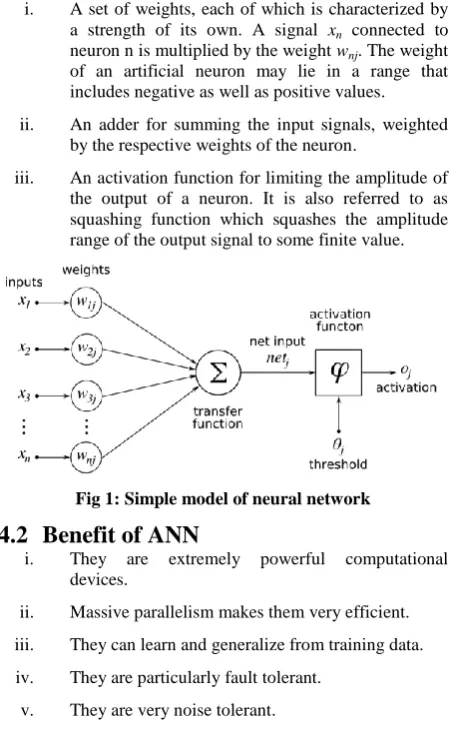
A neuron is an information processing unit that is fundamental to the operation of a neural network. The three basic elements of the neuron model are:
i. A set of weights, each of which is characterized by a strength of its own. A signal xn connected to neuron n is multiplied by the weight wnj. The weight of an artificial neuron may lie in a range that includes negative as well as positive values.
ii. An adder for summing the input signals, weighted by the respective weights of the neuron.
[image:3.595.55.281.297.665.2]iii. An activation function for limiting the amplitude of the output of a neuron. It is also referred to as squashing function which squashes the amplitude range of the output signal to some finite value.
Fig 1: Simple model of neural network
4.2
Benefit of ANN
i. They are extremely powerful computational devices.
ii. Massive parallelism makes them very efficient.
iii. They can learn and generalize from training data.
iv. They are particularly fault tolerant.
v. They are very noise tolerant.
4.3
Network Architecture
There are two fundamental different classes of network architectures:
i. Single layer feed forward network: It has only one layer of computational nodes (output layer). It is a feed forward network since it does not have any feedback. The single layer feed-forward network consists of a single layer of weights, where the inputs are directly connected to the outputs, via a
series of weights. The synaptic links carrying weights connect every input to every output, but no other way. The sum of products of the weights and the inputs is calculated in each neuron node, and if the value is above some threshold (typically 0) the neuron fires and takes the activated value (typically 1); otherwise it takes the deactivated value (typically -1). [3].
Fig 2: Single-layer feed forward network
[image:3.595.341.520.404.498.2]ii. Multi-layer feed forward network: It is a feed forward network with one or more hidden layers. The source nodes in the input layer supply inputs to the neurons of the first hidden layer. The outputs of the first hidden layer neurons are applied as inputs to the neurons of the second hidden layer and so on. If every node in each layer of the network is connected to every other node in the adjacent forward layer, then the network is called fully connected. If however some of the links are missing, the network is said to be partially connected. Recall is instantaneous in this type of network.
Fig 3: Multi-layer feed forward network
4.4
Learning Processes of ANN
By learning rule, we mean a procedure for modifying the weights and biases of a network. The purpose of learning rule is to train the network to perform some task. They fall into three broad categories:
i. Supervised learning: The learning rule is provided with a set of training data of proper network behavior. As the inputs are applied to the network, the network outputs are compared to the targets. The learning rule is then used to adjust the weights and biases of the network in order to move the network outputs closer to the targets.
ii. Reinforcement learning: It is similar to supervised learning, except that, instead of being provided with the correct output for each network input, the algorithm is only given a grade. The grade is a measure of the network performance over some sequence of inputs.
algorithms perform some kind of clustering operation. They learn to categorize the input patterns into a finite number of classes [6].
5.
PROPOSED METHOD
The back-propagation algorithm is used to find a local minimum of the error function. Error back-propagation learning consists of two passes through the different layers of the network: a forward pass and a backward pass. In the forward pass, an input vector is applied to the nodes of the network, and its effect propagates through the network layer by layer. Finally, a set of outputs is produced as the actual response of the network. During the forward pass the weights of the networks are all fixed. During the backward pass, the weights are all adjusted in accordance with an error correction rule. The actual response of the network is subtracted from a desired response to produce an error signal. This error signal is then propagated backward through the network, against the direction of synaptic connections. But before proceeding to the result we require several steps to complete.
5.1
Data Selection
We have used some real data which is representing the record of the power load of Western Part of Saudi Arabia from the year 2003 to 2007. But for our experimental purpose instead of using all the data we have just used three years data from January 2005 to December 2007. Out of which January 2005 to November 2007 is selected for training data and December 2007 is selected for test data. At our real data set we have separate column for the weekdays, but for our experimental ease we have preprocessed the data to count one single column instead of using all seven columns like Saturday is considered as 1, Sunday is 2 and so on.
5.2
Attribute Selection
By trial and error approach, the number of inputs is finalized which is fed to our neural network. At first, we have a separate column for the year, but it is not an important field for our experiment, so the column is been neglected. Similarly, out of total eleven input columns we tried separate combination of input by ignoring one or two columns and checking the test result we have found our best input combination. Dimensionality reduction is very much important for problem solving technique just like our experiment, but by our experiment we found that the best approach is to count all the input columns. The eleven input columns are- 1. Date of the month, 2. Month of the year, 3. Which day of the week, 4. School, 5. Exam, 6. Ramadan, 7. Eid, 8. Hajj, 9. Public holiday, 10. Max temp, 11. Min temp.
5.2.1
Preprocessing of Training Data
The data employed for training and testing the neural network were obtained from the western part of Saudi Arabia and they are real data. All the required input columns value is either 1 or 0 except the date, maximum temperature and minimum temperature column. For our experimental purpose we scaled (dividing by 10) the maximum and minimum temperature. We also tried the normalization technique during our research in order to get a better outcome but it wasn’t happened to be that’s why we neglected the approach of normalization.
5.3
Network Selection
To find a good network for our experiment is essential. As the number of input (11 attributes) and output (Power load) are fixed in the previous steps, so in this step we select the number of hidden layers with the number of neurons in each hidden layer of the individual network. In our approach we
select five networks and the best network which is evaluated based on the average MAPE after 10 runs of the program. In our experiment we use the following combination of network: (No of Input-hidden layers (no of neurons in that layer)-No of output)-> 11-5-1, 11-18-9-4-1, 11-18-7-1, 11-10-10-1, 11-8-1.
In our test we randomly pick the weight and bias of the network and then saved the network for further studies. Thus, each time we load the network it has all the fixed weight and bias which is our requirement. If the weight and bias for a network is fixed then each time the program runs, it will give the same result as it gives at earlier runs.
5.3.1
Train and Test the Network
As we have selected three years record as our dataset, we select our training set data for our experiment from January 2005 to November 2007 i.e. total thirty-five months of record is considered as the training set. Previously we used one-year data as our dataset where eleven months are used as the training set, but the outcome was not fulfilled our expected value. So, instead of taking one year we have taken three years data as our dataset as it is theoretically and practically proved that the classifier’s accuracy is increasing with the increase in the training sample. That is why, instead of taking eleven months we have taken thirty-five months record as our training sample thus a more accurate classification can be made.
Out of thirty-six months of selected dataset, we have used only one month as our test data. December 2007 is selected as our test dataset. When we test the network, we get a forecast set of the test sample which is compared with the actual output to get the result.
5.3.2
Finding MAPE
Mean Average Percentage Error (MAPE) is the final output of our experiment by which we can compare which network and which technique is best fitted for our experiment [7].
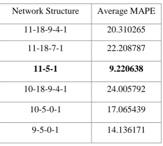
where At is the actual value and Ft is the forecast value. In this way by running the program for ten times for each network we get the network which has the lowest average MAPE. That network is selected for further experiment. Some of the networks are shown in the following Table 1.
The best neural network 11-5-1 is taken into account to obtain the forecast value and thus calculate the MAPE which is represented in Fig. 4.
5.4
Creating Clone Network
The network which is selected by trial and error approach of the previous steps are then taken to create ten versions of that similar network structures only the weight and bias are randomly generated. Still all the networks are saved for the coming experiment.
5.4.1
Train the Clone Network Individually
After loading the already saved clone network it is then trained by the train set as earlier i.e. thirty-five months records. These steps will operate for each ten cloned networks one by one and will ready to perform the next sequential steps. Just like the previous testing approach the cloned network is then tested by the test set.
While training the cloned version of the network its attributes are assigned with the values which is required to save for the further experiment. So, after the training all the data which are essential for the study are saved. These networks are then feed to the clustered data which is also a criterion for our experiment.
Table 1. Best network selection
Network Structure Average MAPE
11-18-9-4-1 20.310265
11-18-7-1 22.208787
11-5-1 9.220638
10-18-9-4-1 24.005792
10-5-0-1 17.065439
9-5-0-1 14.136171
5.4.3
Test the Clone Network
Just like the previous testing approach the cloned network is then tested by the test set.
5.4.4
Calculate MAPE
MAPE calculation for the selection of the best network as earlier is then used for the MAPE calculation of the cloned network. The new forecasted data which is collected after the testing are taken into account to compute the MAPE.
Fig 4: Forecasted value with absolute error of the NN approach
5.5
Cluster Selection
From our training dataset we have clustered the data into three groups. For our clustering we have chosen k-means clustering technique. Before the clustering to implement we have decided we will divide the training data into three cluster and then proceed for further analysis. We have chosen the centroid based built in k-means function of MATLAB to determine the clustered data. Only the maximum and minimum temperature are considered for the condition of clustering criteria. The training dataset are then grouped into three different cluster set checking the outcome of the k-means output.
Then the test set i.e. 31 data are then divided into three clustered on the basis of the three centroids which is found while the built-in k-means clustering function is called.
5.5.1
Load Each Cloned Network One-by-one
After the clustering has done then each cloned network is loaded one by one. As the weight and bias and other attributes are same as previous only the training and test set are different now.
5.5.2
Train the Network
The loaded network is tested separately by three test set which are divided based on cluster in the previous step. The training technique is same as the previous one.
5.5.3
Test the Network
Just like training of the three clustered set, three clustered test set is then simulated separately for the forecasted value which is then compared with the corresponding record of the actual output to compute the result.
5.5.4
Calculate MAPE
Just like the previous MAPE calculation the MAPE is calculated for the k-means clustering technique and record it into the excel sheet. All the processes are run ten times and then get the average MAPE. Combined forecasted value of the three clusters together with absolute error is shown in Fig. 5.
[image:5.595.314.543.297.473.2]Fig 5: Forecasted value with absolute error of the clustering approach
5.6
Experimental Results
In this paper, we try to find the best clustering method for grouping the load consumption data in order to improve the accuracy of load forecasting at the network level. Moreover, we introduce a new method for aggregating the forecast load for each cluster to derive a network level load forecast that is more accurate than previous methods. Fig 6 represents the visual representation of the actual load comparison and Fig 7 shows the percentage error of the two approaches. And we can easily understand that the clustering technique is the best approach which is suited ours experiment.
The result shows that our proposed model has a good performance and reasonable prediction accuracy can be achieved. Its forecasting reliabilities are evaluated by computing the mean absolute error between the exact and predicted values. We are able to obtain MAPE of 20.4138% which represents a reasonable degree of accuracy. Table 2. demonstrates the comparison among the three techniques in our entire research.
0 1000 2000 3000 4000 5000 6000 7000 8000
1 3 5 7 9 11 13 15 17 19 21 23 25 27 29 31
Lo
ad
Day
Actual Forecast Absolute Error
0 2000 4000 6000 8000 10000
1 3 5 7 9 11 13 15 17 19 21 23 25 27 29 31
Lo
ad
Day
[image:5.595.53.283.399.560.2]6.
CONCLUSION AND FUTURE WORK
[image:6.595.307.549.68.502.2]The results obtained from testing the trained neural network for one month data using ANN STLF model shows that the ANN Model has been given good performance and reasonable prediction accuracy was achieved. In addition, we show that by using an appropriate clustering method we can further improve forecasting accuracy. The results suggest that ANN model with the developed structure can perform good prediction with least error and finally this neural network with clustering. So, it can be an important tool for short term load forecasting.
[image:6.595.52.281.195.358.2]Fig 6: Actual load comparison of the two approaches
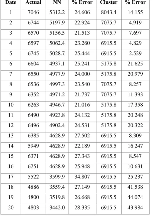
Table 2. Final forecasted value with respective MAPE of the two approaches
Date Actual NN % Error Cluster % Error
1 7046 5312.2 24.606 8043.4 14.155
2 6744 5197.9 22.924 7075.7 4.919
3 6570 5156.5 21.513 7075.7 7.697
4 6597 5062.4 23.260 6915.5 4.829
5 6745 5028.7 25.444 6915.5 2.529
6 6604 4937.1 25.241 5175.8 21.625
7 6550 4977.9 24.000 5175.8 20.979
8 6536 4997.3 23.540 7075.7 8.257
9 6352 4971.2 21.737 7075.7 11.393
10 6263 4946.7 21.016 5175.8 17.358
11 6490 4923.8 24.132 5175.8 20.248
12 6496 4902.4 24.531 5175.8 20.322
13 6385 4628.9 27.502 6915.5 8.309
14 5949 4628.9 22.189 6915.5 16.247
15 6371 4628.9 27.343 6915.5 8.547
16 6251 4628.9 25.948 6915.5 10.631
17 5522 3599.9 34.807 6915.5 25.237
18 4886 3559.4 27.149 6915.5 41.538
19 4800 3519.8 26.668 6915.5 44.074
20 4803 3442.0 28.335 6915.5 43.984
21 4565 3351.9 26.573 5175.8 13.381
22 4860 3812.5 21.552 6915.5 42.296
23 5124 4628.9 9.661 6915.5 34.964
24 5182 4628.9 10.672 6915.5 33.454
25 5230 4628.9 11.492 6915.5 32.229
26 5367 4628.9 13.751 6915.5 28.853
27 5402 4628.9 14.310 6915.5 28.019
28 5555 4435.8 20.147 6915.5 24.493
29 6040 4734.4 21.614 6915.5 14.496
30 6054 4743.9 21.639 6915.5 14.231
31 6092 4723.2 22.468 6915.5 13.519
MAP
E 22.446 20.4138
MIN 9.661 2.529
MAX 34.807 44.074
Fig 7: Percentage error comparison of two approaches
7.
REFERENCES
[1] Zhang, Mi & Xia, Changhao. (2017). A Loose Wavelet Nonlinear Regression Neural Network Load Forecasting Model and Error Analysis Based on SPSS. International Journal of Information Technology and Computer Science. 9. 24-30. 10.5815/ijitcs.2017.04.04.
[2] Yasser Al-Rashid and Larry D. Paarmann, “Short –Term Electric Load Forecasting Using Neural Network Models”, 0-7803-3636-4/97, 1997 IEEE.
[3] P. Fishwick, ”Neural network models in simulation: A comparison with traditional modeling approaches,” Working Paper, University of Florida, Gainesville, FL,1989.
[4] https://www.worldometers.info/world-population.
[5] Sannella, M. J. 1994 Constraint Satisfaction and Debugging for Interactive User Interfaces. Doctoral Thesis. UMI Order Number: UMI Order No. GAX95-09398., University of Washington.
[6] P. Werbos, “Generalization of backpropagation with application to recurrent gas market model”, Neural
0 2000 4000 6000 8000 10000
1 3 5 7 9 11 13 15 17 19 21 23 25 27 29 31
Lo
ad
Day
Actual NN Cluster
0 10 20 30 40 50
1 3 5 7 9 11 13 15 17 19 21 23 25 27 29 31
%
E
rro
r
Day
[image:6.595.46.291.411.760.2]Networks, vol.1,pp.339 – 356,1988.
[7] K.Y. Lee, Y.T. Cha and J.H. Park, “Short Term Load Forecasting Using an Artificial Neural Network”, IEEE Transactions on Power Systems, Vol 1, No 1, February 1992.
[8] Mohsen Hayati and Yazdan Shirvany, “Artificial Neural Network Approach for Short Term Load Forecasting for Illam Region”, International Journal of Electrical Computer and System Engineering Volume 1, Number 2, 2007 ISSN 1307-5179.
[9] “Load Forecasting” Chapter 12, E.A. Feinberg and Dora Genethlio, P 269–285, from links: www.ams.sunysb.edu and www.usda.gov.
[10] G.A. Adepoju, S.O.A. Ogunjuyigbe and K.O. Alawode, “Application of Neural Network to Load Forecasting in Nigerian Electrical Power System”, Volume 8, Number 1, May 2007 (Spring).
[11] Lru, K., Subbarayan, S., Shoults, R.R., Manry, M.T., Kwan, C., Lewis, F.L. and Naccarino, J., “Comparison of very short term load forecasting techniques,” IEEE Trans. Power Syst., 11(2): 877-882, May (1996).
[12] Ahmad A., Anderson T.N., Rehman S.U. (2018) Prediction of Electricity Consumption for Residential Houses in New Zealand. In: Chong P., Seet BC., Chai M., Rehman S. (eds) Smart Grid and Innovative Frontiers in Telecommunications. SmartGIFT 2018. Lecture Notes of the Institute for Computer Sciences, Social Informatics and Telecommunications Engineering, vol 245. Springer, Cham.
[13] Senjyu, T., Mandal, P., Uezato, K. and Funabashi, T., “Next day load curve forecasting using hybrid correction method”, IEEE Trans. Power Syst., 20(1), Feb. (2005). [14] Rahman, S. and Hazim, O., “A generalized
knowledge-based short term load forecasting technique”, IEEE Trans. Power Syst., 8(2): 508-514, May (1993).
[15] Ho, K.L., Hsu, Y.Y., Liang, C.C. and Lai, T.S., “Short-term load forecasting of Taiwan power system using a knowledge-based expert system”, IEEE Trans. Power Syst.,5(4), Nov. 1990.
[16] K.-H. Kim, J.-K. Park, K.-J. Hwang, and S.-H. Kim, “Implementation of hybrid short-term load forecasting system using artificial neural networks and fuzzy expert systems,” IEEE Transactions on Power Systems, vol. 10, no. 3, pp. 1534–1539, 1995.
[17] P.-F. Pai and W.-C. Hong, “Support vector machines with simulated annealing algorithms in electricity load forecasting, Energy Conversion and Management, vol. 46, no. 17, pp. 2669–2688, 2005.
[18] T. M. Cover and P. E. Hart, “Nearest neighbor pattern classification,” IEEE Transactions on Information Theory, vol. 13, no. 1, pp. 21–27, 1967.
[19] Baklrtzis, A.G., Petrldis, V., Klartzis, S.J., Alexiadls, M.C. and Malssis, A.H., “A neural network short term load forecasting model for the Greek power system,” IEEE Trans. Power Syst., 11(2): 858-863, May (1996).
[20] Yu-Jun He; You-Chan Zhu; Jian-Cheng GU; Cheng-Qun
Yin; Similar day selecting based neural network model and its application in short term Load forecasting, Proceedings of International Conference on Machine Learning and Cybernetics; Aug. 2005. vol. 8, p.4760-4763.
[21] M. B. Abdul Hamid and T. K. Abdul Rahman. Short Term Load Forecasting Using an Artificial Neural Network Trained by Artificial Immune System Learning Algorithm, 12th International Conference on Computer Modeling and Simulation (UKSim), 2010, p. 408-413.
[22] Hernández, Luis & Baladrón, Carlos & M Aguiar, Javier & Calavia, Lorena & Carro, Belén & Sánchez-Esguevillas, Antonio & Cook, Diane & Chinarro, David & Gómez-Sanz, Jorge. (2012). A Study of the Relationship between Weather Variables and Electric Power Demand inside a Smart Grid/Smart World Framework. Sensors (Basel, Switzerland). 12. 11571-91. 10.3390/s120911571.
[23] EI Desouky, A, Aggarwal, R., Elkateb, M., Li, F., Advanced hybrid Genetic algorithm for short-term generation scheduling. IEEE Proceedings Generation, Transmission and Distribution 2001. 148 (6), p. 511-517.
[24] Liao, G.-c., Tsao, I.-P., Application of a fuzzy neural network combined with a chaos genetic algorithm and simulated annealing to short-term load forecasting. IEEE Transactions on Evolutionary Computation 2006. (3), p.330-340.
[25] Heng, E.T.H.; Srinivasan, D.; Liew, A.C.;, Short term load forecasting using genetic algorithm and neural networks, Energy Management and Power Delivery, 1998. Proceedings of EMPD '98. 1998 International Conference on, 3-5 Mar 1998.Vol. 2, no., p. 576-581.
[26] Sudhansu Kumar Mishra, Ganapati Panda and SukadevMeher. “Multiobjective Particle Swarm Optimization Approach to Portfolio Optimization” IEEE, World Congress on Nature and Biologically Inspired Computing (NaBIC-2009), Coimbatore, India. 09-11 December 2009, pp.1612-1615.
[27] Sudhansu Kumar Mishra, Ganapati Panda and SukadevMeher, RitanjaliMajhi,“Comparative Performance Study of Multiobjective Algorithms for Financial Portfolio Design” International Journal of Computational Vision and Robotics, Inderscience publisher. Vol. 1, No.2, pp.236- 247, 2010.
[28] Tian Shu, Liu Tuanjie. Short Term Load Forecasting Based on RBFNN and QPSO,Power and Energy Conference, 27-31 March 2009.p. 1-4.
[29] Ning Lu; Jianzhong Zhou;, Particle Swarm Optimization-Based RBF Neural Network Load Forecasting Model, Power and Energy Engineering Conference, APPEEC 2009, 27-31 March 2009. Asia-Pacific, p. 1-4.