Experiments on the Self Organized Critical State of 4He

(1)

Thesis by

Andrew Rosenberg Chatto

In Partial Fulfillment of the Requirements

for the Degree of

Doctor of Philosophy

California Institute of Technology

Pasadena, California

2006

(2)

ii

c

2006

Andrew Rosenberg Chatto

(3)

Acknowledgements

There are a number of people I would like to thank for their contributions to this thesis. My advisor

David Goodstein was insightful, encouraging, and patient throughout the many challenges of

per-forming a low-temperature experiment. Our conversations were always helpful because David has

an extraordinary ability to make complicated concepts seem simple and intuitive. I had two mentors

in the lab, Peter Day and Richard Lee, who taught me everything I know about performing

exper-iments in low-temperature physics. My first lab experience was working with Peter. He provided

me with the cryostat I used throughout my graduate career, answered hundreds of questions, and

patiently showed me the techniques I needed. Richard returned to Caltech as my thesis experiment

was taking shape. He was also an excellent resource for the tricks and techniques of low-temperature

physics. (Plus, he made B.O.B.2, the electrical filtering system on this cryostat). However, what

helped me most was that he patientlyaskedhundreds of questions, which forced me to think through

all the details of my experiment. It is with his help that I avoided many pitfalls.

There are a number of other physicists who made significant contributions to this work.

Partic-ularly helpful were the members of the DYNAMX team from the University of New Mexico (Rob

Duncan, Dimitri Sergatskov, Alex Babkin, and Steve Boyd). They provided material help with the

cryo-valve system and the construction of the experimental cell. In addition, they provided a lot of

expertise on performing experiments on the SOC state of 4_{He. In particular, I would like to thank}

Rob Duncan, who served as a secondary thesis advisor during a critical time in the experiment as

David Goodstein recovered from an injury. Also helpful were discussions with two theorists, Peter

Weichman and Rudolf Haussmann, who helped give meaning to my results.

I would like to thank my parents for many many years of encouragement and support, and not

asking me too often when I was going to get my degree.

I would also like to thank my wife Avital, who provided an enormous amount of support and,

through an intricate dance of prodding and patience, helped guide me through this endeavor. Lastly,

I thank my son Jacob, whose arrival helped destroy the illusion that maybe, just maybe, I could be

(4)

iv

Abstract

When a heat flux is applied downwards through a sample of4_{He near the superfluid transition}

tem-peratureTλ, the gradient in the temperature self-organizes to the gradient inTλcaused by gravity.

This creates the Self-Organized Critical (SOC) state. Previous experiments have observed the state,

measured the self-organization temperatureTSOC vs. heat flux, and investigated a remarkable wave

that only travels upwards against the flow of the heat flux [1, 2, 3].

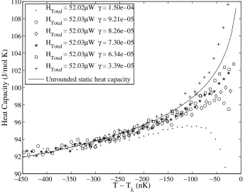
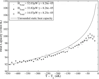
We report the first results of the heat capacity of the SOC state,C∇_T, for heat fluxes 60nW/cm2<

Q <13µW/cm2_{and corresponding temperatures 9 nK}_{> T}

SOC−Tλ>−1.1µK. We find thatC∇_T

tracks the static (i.e., zero heat flux) unrounded (i.e., in zero gravity) heat capacity C0 with two

exceptions. The first is that within 250 nK ofTλ,C∇T is depressed relative toC0 and the maximum

inC∇T is shifted to 50 nK belowTλ. The second difference is that at high heat flux,C∇T is again

depressed relative toC0with the departure starting at about 650 nK belowTλ.

We present the most extensive measurements of the speed and attenuation of the SOC wave to

date. We report wave speed measurements taken over our full experimental range 30 nW/cm2 <

Q <13µW/cm2_{and attenuation results over the limited range that produced enough attenuation}

(5)

List of Tables

3.1 Resistances of the thermal network . . . 21

3.2 Heater calibrations . . . 22

3.3 Heat capacities of the endplates . . . 23

3.4 HRT calibrations . . . 27

3.5 HRT noise . . . 29

3.6 Kapitza resistances . . . 31

3.7 Moles in helium sample . . . 41

4.1 Parameters for SOC heat capacity runs . . . 58

(9)

List of Figures

1.1 Profiles of the SOC state . . . 2

1.2 Schematic of the staircase SOC state profile . . . 3

1.3 Haussmann’s prediction forC∇T compared to the static heat capacity . . . 4

2.1 Schematic of the cryostat . . . 10

2.2 Schematic detail of the stages . . . 12

2.3 Mounting platform schematic . . . 13

2.4 Schematic of the heater control . . . 17

3.1 Top endplate response to heat pulse . . . 22

3.2 Bottom endplate response to heat pulse . . . 23

3.3 Cell temperature profiles when the bubble is inside the cell . . . 26

3.4 Calibration of HRTT. . . 27

3.5 Calibration of HRTM . . . 28

3.6 Calibration of HRTB . . . 28

3.7 Noise of HRTT . . . 29

3.8 Noise of HRTM . . . 30

3.9 Noise of HRTB . . . 30

3.10 Heater response time . . . 32

3.11 Measurement of cell heater response time . . . 34

3.12 Dependence of GRT bottom on heat flux . . . 35

3.13 Midplane temperature offset . . . 37

3.14 Pulse heat capacity results . . . 38

3.15 Temperature step oscillation . . . 39

3.16 Heat capacity results with a 3.98µJ pulse size . . . 40

3.17 Volume calibration schematic . . . 40

4.1 Schematic of the temperature profiles during the SOC state heat capacity measurement 44 4.2 SOC heat capacity time series data . . . 44

(10)

x

4.4 SOC heat capacity results for different foil heats . . . 51

4.5 SOC heat capacity results to determine the foil heat factorγ . . . 52

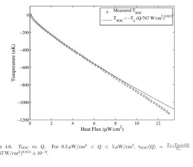
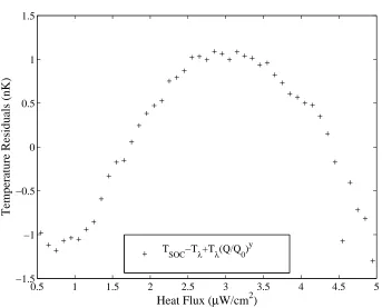
4.6 TSOC vs.Q . . . 53

4.7 TSOC vs.Qfit residuals . . . 54

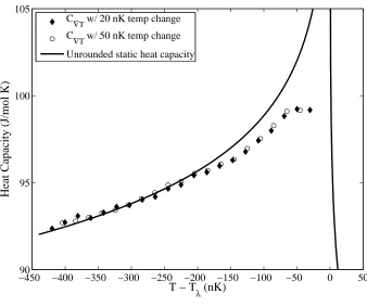
4.8 SOC heat capacity with different temperature steps ∆TSOC . . . 55

4.9 SOC heat capacity with different ramping heatsδH . . . 56

4.10 The effect of imbalance on the SOC heat capacity . . . 57

4.11 SOC heat capacity . . . 59

4.12 Log-log plot of SOC heat capacity . . . 60

4.13 SOC heat capacity results compared to Haussmann’s prediction . . . 61

4.14 Log-log plot of SOC heat capacity results compared to Haussmann’s prediction . . . . 62

5.1 Comparison of HRTTto a reference sine wave . . . 64

5.2 Amplitude vs. reference sine wave phase shift . . . 65

5.3 HRTTphase delay and HRTM phase delay vs. HRTT . . . 66

5.4 Second sound correction of HRTTphase delay . . . 68

5.5 Attenuation of the SOC wave amplitude . . . 69

5.6 Wave speed vs. heat flux . . . 70

5.7 TSOC vs.Qfit residuals using a fourth-degree polynomial . . . 71

5.8 Wave speed vs. heat flux results compared to theory . . . 72

5.9 Attenuation . . . 73

5.10 Extracting thermal conductivity fromTSOC vs.Qfit residuals . . . 74

5.11 Scaled attenuation length vs. heat flux . . . 76

5.12 Scaled attenuation length vs. the attenuation length . . . 77

5.13 Incorrectly scaled attenuation length vs. heat flux . . . 78

6.1 TSOC vs.Q . . . 80

6.2 TSOC vs.Qfit residuals . . . 80

6.3 SOC heat capacity . . . 81

6.4 Wave speed vs. heat flux . . . 82

6.5 Scaled attenuation length vs. attenuation length . . . 83

A.1 A photo of the cell stage . . . 88

A.2 A CAD rendering of the cell stage . . . 89

A.3 The bottom endplate . . . 90

A.4 The top endplate . . . 91

(11)

A.6 The middle piece of the Vespel sidewall . . . 93

A.7 The top piece of the Vespel sidewall . . . 94

A.8 The sidewall foil . . . 95

A.9 The cap for attaching the fill line to the sidewall . . . 96

A.10 The titanium mounting plate . . . 97

A.11 The heat sinking foil . . . 98

A.12 The heat conduction foil . . . 99

A.13 The bubble chamber . . . 100

A.14 The cap for the bubble chamber . . . 101

A.15 Vespel thermal standoff for the bubble chamber and cryo-valve . . . 102

A.16 Vespel mount for the bubble chamber and cryo-valve . . . 103

(12)

(13)

Chapter 1

Introduction

The Self-Organized Critical (SOC) state in4_{He is a peculiar phenomenon arising when a heat flux}

is applied downwards through a sample of helium near the superfluid phase transition. Below the

superfluid transition, helium has virtually no gradient under an applied heat flux as long as the

heat flux does not exceed some critical value. Above the transition, the helium conducts heat as a

typical fluid, although near the transition the thermal conductivity is significantly enhanced. Under

certain conditions, when a heat flux is applied downwards, the helium self-organizes to a gradient

of 1.273µK/cm independent of the heat flux. This state is phenomenally robust; it has been seen

over more than 2 orders of magnitude in heat flux (from 40 nW/cm2_{to 6}_.₅_µ_W_/_cm2_{) [1].}

1.1

The SOC State

The superfluid transition temperature,Tλ, is depressed from its value at SVP by an imposed pressure.

Therefore, a sample of helium on the surface of the Earth always has a gradient in the transition

temperature ofdTλ/dz= 1.273µK/cm. AboveTλbut near the transition, the thermal conductivity

is determined by the proximity to Tλ [4]. Therefore, if we define the reduced temperature t(z) = T−Tλ(z)

Tλ , regions with the same reduced temperature will have the same conductivity.

Suppose we have a heat flux flowing downwards through a sample of helium. While in the

superfluid, there will be no thermal gradient as in profileAof fig. 1.1. If we allow the entire sample

to slowly warm, eventually the temperature at the bottom of the sample will passTλ(z = 0) and

will begin to form a gradient.1 _{As the sample warms, the gradient will continue to get larger until}

it matches the gradient inTλ as shown by profileB. The region of the helium where the gradient

matches the gradient inTλis in the SOC state. As the sample continues to warm, more helium will

transition into the SOC state and profileCwill be reached. When profile Dis reached, the entire

sample is in the SOC state and has the same reduced temperaturet. As the sample warms further,

a region of high gradient normal fluid will be created at the top of the sample as in profileE. The

1_{Actually, the gradient starts to form when the temperature passes}_T

C(Q, z)≃Tλ(z)−Tλ Q/784 W/cm2

0.813

(14)

[image:14.612.188.387.53.254.2]

2

Figure 1.1. Profiles of the SOC state.

process continues as less and less helium remains in the SOC state and the high gradient normal

fluid occupies more and more of the sample. Eventually, if we allow the sample to continue to warm,

the arrangement will become unstable as the very warm helium at the top of the sample becomes

more dense than the helium in the SOC state and convection disturbs our quasi-equilibrium.

The SOC state for normal He-I as described above was predicted by Onuki in 1987 [5].

Exper-iments to observe the state were conducted at the University of New Mexico by Moeur et al. and

published in 1997 [1]. They saw the expected self-organization at low heat fluxes, but continued to

see the SOC state for higher heat fluxes, with a self-organization temperature belowTλ. They

pre-sented a phenomenological model that treated the SOC state helium both above and belowTλas a

normal fluid with a thermal conductivity that diverged not atTλbut at a temperatureTC(Q)< Tλ.

They gave the thermal conductivityκas

κ(T, Q) =κ0

_T

−TC(Q)

Tλ

−x

(1.1)

withTC(Q) =Tλ−Tλ(Q/Q0)0.813. In the SOC state, the temperature gradient equals the gradient in Tλ, giving κ = ∇Tλ/Q. They used this to extract the following values for the parameters:

κ0 = 294 nW/cm K, x= 0.664, and Q0 = 638 W/cm2. One can make an extrapolative leap and

propose that thisTC(Q) is actually a depressedTλ(Q) and a true critical point. As we go to larger

and larger heat flux, we need a higher thermal conductivity so the SOC temperature moves closer

and closer to this critical point. We already have evidence that the conductivityκis diverging here.2

2

In this instance, we have actually definedTC(Q) as the temperature whereκ diverges. A previous experiment

(15)

Figure 1.2. Schematic of the staircase SOC state profile in the Weichman and Miller model [7].

If we could examine other quantities as we approachedTC(Q), such as the heat capacity, we could

test the hypothesis thatTC(Q) is a critical point.

Following these interesting experimental results, Weissman and Miller examined the SOC state

below Tλ through a one-dimensional mean-field model [7]. They calculated that it was possible to

have an superfluid SOC state below Tλ through a regular series of slips of the phase of the order

parameter. These phase slips lead to a staircase-like temperature profile that, when viewed on a

macroscopic scale, appears as a smooth temperature gradient. This is represented schematically in

fig. 1.2. The main difference of this model contrasted with the proposal of a depressedTλ(Q) is that

the helium is essentially a superfluid. Viewed as a whole, the helium appears as normal fluid with a

uniform gradient. However, viewed on small length scales, the majority of the helium is a superfluid

with no gradient.

1.2

The SOC Heat Capacity

Near the superfluid phase transition temperatureTλ, the static heat capacity (i.e., the heat capacity

without a heat flux, SOC inducing or not) is dominated by the energy contribution of the random

fluctuations between the two phases of helium, He-II (superfluid) and He-I (normal fluid).3 _Since

there is no latent heat for the phase transition, the free energy difference between the two phases

goes to zero as one approachesTλand the fluctuations between them get larger and more numerous.

These fluctuations give rise to a singularity in the heat capacity ofC∼t−α_where_α_{≃ −}₀_._13.

Rudolf Haussmann used dynamic renormalization group theory to calculate the heat capacity of

the SOC state, C∇T [9]. A plot of his results close to Tλ are given in fig. 1.3. More than 100 nK

3_{For more details on the critical point phenomena near}_T

(16)

4

−600

75

−500

−400

−300

−200

−100

0

100

80

85

90

95

100

105

110

T − T

_λ

(nK)

Heat Capacity (J/mol K)

Unrounded static heat capacity

Haussmann C

_∇

T

Figure 1.3. Haussmann’s prediction forC∇_T compared to the zero-gravity static heat capacity.

away from Tλ, the heat capacity is the same as in the zero-gravity static case. Very close to Tλ,

however, the heat capacity is significantly depressed and the maximum is shifted to 50 nK below

Tλ.

Another prediction forC∇T comes from the suggestion thatTC(Q) might be the depressed critical

point Tλ(Q) with a thermal conductivity of the form given in eq. (1.1). Under this assumption,

TSOC(Q) for low Qis far from the critical point. As Q is increased, however,TSOC(Q) gets closer

and closer to TC(Q). Therefore, as we approach the critical point TC(Q) from above, we would

expect the heat capacity to diverge as in the static case.

It is also possible that dynamic effects of the two-fluid model could play a role in the heat capacity.

In traditional helium under a heat flux, there is predicted a contribution to the heat capacity from

the kinetic energy of the flow of the superfluid [10], which has been observed experimentally in a

“heat-from-below” configuration [11]. However, it is unclear whether this mechanism would apply

(17)

1.3

The SOC State Wave

In investigating the SOC state for temperatures aboveTλ, Weichman and Miller also predicted the

existence of a thermal wave that would travel only upstream against the flow of the heat flux [7].

However, this wave has been seen experimentally by Sergatskov et al. both above and belowTλ [2].

To understand the nature of this wave, we will treat the helium as a normal fluid with a conductivity

κthat is a function of both the temperature and the heat flux. This appears to be in contradiction

to the work of Weichman and Miller who treated the high heat flux SOC state as a superfluid with

a regular occurrence of phase slips. Nevertheless, we will press on and defer judgment as to the

validity of this approach until its predictions are compared with experimental measurements. This

calculation roughly follows the calculation that Sergatskov et al. provided with their experimental

paper [2].

We start with the regular heat transfer equations,

C∂T

∂t =−∇ ·~ Q~ (1.2)

and

~

Q=−κ~∇T. (1.3)

Since the wave travels upwards and the nominal heat flux is downwards, we restrict ourselves to the

z axis. We define the heat flux to be positive by settingQ~ =−Qzˆand defineQSOC as the nominal heat flux of the SOC state. We combine eqs. (1.2) and (1.3) to get

C∂T ∂t = ∂ ∂z κ∂T ∂z . (1.4)

Next, we transform to the reduced temperatureǫ= (T−Tλ)/Tλ. First, we compute the derivative

∂T ∂z =Tλ

∂ǫ

∂z+α (1.5)

whereα= dTλ

dz = 1.273µK/cm. Then we convert eq. (1.4) to get

CTλ∂ǫ

∂t = ∂ ∂z κ

Tλ∂ǫ

∂z +α

(1.6)

At this point, we will avoid making the assumption thatκis of the form given in eq. (1.1). We

will, however, assume that the thermal conductivity is a function of onlyǫandǫ′

= _∂z∂ǫ. This leads

to

CTλ∂ǫ

∂t = ∂κ ∂ǫ ∂ǫ ∂z + ∂κ ∂ǫ′ ∂ǫ′ ∂z Tλ

∂ǫ ∂z+α

+κTλ∂

2_ǫ

∂z2. (1.7)

(18)

6

are squared to get

CTλ

∂ǫ ∂t =α

∂κ ∂ǫ ∂ǫ ∂z+ α∂κ ∂ǫ′ +κTλ

_∂2_ǫ

∂z2. (1.8)

We guess that there is a wave of the form

ǫ(z, t) = ǫ0+δ(z, t) (1.9)

= ǫ0+δ0e

−Dk2

t_eik(z−vt)_. _(1.10)

Putting in the trial solution gives

CTλ −Dk2−ikv=α∂κ

∂ǫ(ik) +

α∂κ ∂ǫ′ +κTλ

(ik)2. (1.11)

From the real parts, the attenuation is given by

D= κ

C + α CTλ

∂κ

∂ǫ′. (1.12)

(Note, if we had ignored theǫ′

dependence ofκwe would have gottenD= _Cκ.) From the imaginary

parts, the velocity is given by

v=−_CTα

λ

∂κ

∂ǫ. (1.13)

It is important to note that since ∂κ_∂ǫ <0, v is positive and the wave travels upstream against the

heat flux that maintains the SOC state.

We can transform the expression for the velocity into a more easily measured quantity by using

the simple expression for the SOC state thermal conductivity,κ= QSOC

α , whereQSOCis the nominal

heat flux of the SOC state. This is, of course, not strictly true in the case where there is a traveling

wave, but any correction will be small becauseTλ_∂z∂ǫ ≪α. Taking the derivative gives

∂κ ∂ǫ =

Tλ

α

∂QSOC

∂T , (1.14)

where ∂QSOC

∂T is easily extracted by measuringTSOC as a function ofQ. Substituting into eq. (1.13) gives an alternate expression for the velocity

v=−_C1 ∂Q_∂TSOC. (1.15)

We cannot explore the thermal conductivity as a function of the temperature gradient because

the gradient is fixed by gravity. Instead, we will need to make additional assumptions to make any

(19)

assume the thermal conductivity is of the form

κ=κ0θ−x (1.16)

where

θ=ǫ+ (Q/Q0)y. (1.17)

Remembering that the heat flux is given by

Q=κ∂T ∂z =κ

α+Tλ∂ǫ

∂z

, (1.18)

we take the derivative with respect toǫ′

to get

∂κ

∂ǫ′ = − xκ

θ ∂θ

∂ǫ′ (1.19)

= −xκ_θ _Qy

Q Q0

y

∂Q

∂ǫ′ (1.20)

= −_θαxy

Q Q0

y

α∂κ ∂ǫ′ +Tλ

∂ǫ ∂z

∂κ ∂ǫ′ +Tλκ

. (1.21)

We drop the second term in the rightmost grouping because it is much smaller than the first, given

Tλ_∂z∂ǫ ≪α. This gives us

∂κ ∂ǫ′ =−

xy θ Q Q0 y ∂κ ∂ǫ′ +

Tλκ

α

. (1.22)

We solve for ∂κ ∂ǫ′ to get

∂κ ∂ǫ′ =−

Tλκ

α

1 + θ xy

Q Q0

−y. (1.23)

This give us a model-dependent expression for the attenuation of

D= κ

C



 1−

1

1 + θ xy Q Q0 −y  

. (1.24)

It is worth exploring both the low and highQlimits before we have the data to plug in actual values

forx,y, and θ(Q). In the lowQlimit,Q−_y

grows very large and we obtain

lim

Q→0D=

κ C ≃

Q

αC. (1.25)

In the highQlimit,κbecomes large and thereforeθis small, giving

lim

(20)

8

It is not immediately apparent whether this grows or shrinks as Q becomes large. Therefore, we

substituteθ= (κ/κ0)−1/xandκ=Q/αto get

lim

Q→∞D = Q αC 1 xy Q ακ0

−1/x

Q Q0

−y

(1.27)

= (ακ0) 1/x_Q

0y

αCxy Q

(1−₁_/x−_y₎

. (1.28)

Therefore, ify+ 1/x >1, the dissipation of the SOC wave will go to zero for high heat flux. Since

a previous experiment gavey= 0.813 andx= 0.663 [1], we expect little to no attenuation for high

heat flux. If, instead, we had ignored the dependence ofκon the temperature gradient, we would

have predicted thatD= _αCQ and that the dissipation would grow larger with heat flux.

Our answers differ from those of the calculation by Sergatskov et al. for two reasons. First,

they modeledκas we did in eqs. (1.16) and (1.17). However, they computed ∂κ ∂ǫ

Q, treatingQas

constant. This gave them a wave speed v ∼Q3.3_{. However, a change in} _κ _{results in a change in} heat flux. Therefore, the derivative cannot be taken keeping the heat flux constant. We avoided

this problem by transforming our derivative from ∂κ_∂ǫ to Tλ

α ∂QSOC

∂T . If we assume, as they did, that

ǫSOC∼Q0.813, we getv∼Q0.167. Second, in the Sergatskov paper, they ignored the dependence of the thermal conductivityκon the gradient in reduced temperature. As noted above, this causes an

overestimate in the dissipation, especially for high heat flux. With these modifications, we calculate

a very different velocity and attenuation for the SOC wave at all but the lowest heat fluxes.

1.4

Summary

Some of the questions brought up in this introduction are the following:

• Is TSOC(Q) a true critical point?

• Is Haussmann’s calculation of C∇T accurate?

• Can a treatment of the SOC state thermal conductivity as a function of reduced temperature and its derivative accurately predict the speed and attenuation of the SOC wave?

In order to answer these questions, we have measured C∇T, TSOC vs. heat flux Q, and the speed

and attenuation of the SOC wave. Before discussing those measurements, it is necessary to describe

(21)

Chapter 2

Apparatus

The requirements for doing experiments on the SOC state are similar to those of most other 4_He

lambda point experiments. We need an experimental platform with a very stable temperature and

heat flux at the lambda point. We want to investigate heat fluxes in the range of 30 nW/cm2 _to

10µW/cm2_{. The range in SOC state temperatures of these heat fluxes is only 1}_µ_{K. We therefore}

need subnanokelvin temperature measurement precision and subnanowatt heat flux stability.

2.1

Cryogenic System

A schematic of the dewar and probe insert is presented in Fig 2.1. It is a typical cryostat for this

application. The dewar has a waist to give a long hold time between transfers of approximately six

days for a relatively short dewar only four feet tall. It is surrounded by aµ-metal shield to screen out

magnetic fields. The dewar is attached at the top to an aluminum platform (not pictured), which is

supported from the floor by three air legs to reduce vibration. Ironically, the aluminum plate that

is so carefully isolated from vibration has three large cavities that act as organ pipes and vibrate

sympathetically with the noises in the lab. It was not until my ear happened to be close to one end,

and I heard the clear tone, that I discovered the source of some of our vibrational noise. Once the

cavities were filled with foam, this vibration was significantly reduced.

The probe insert is composed of a brass top plate, stainless steel support tubes and an aluminum

vacuum can. There are copper baffles to limit radiative and convective warming. Just inside the

vacuum can there is a 1 K pot to provide cooling of the experiment below 4 K. It has a

high-impedance inlet that passes through a filter. In addition, there is a pump line for the vacuum can,

a pump line for the 1 K pot and conduits for the four SQUID leads.

The probe has 56 manganin wires arranged in twisted pairs. At the top of the probe, these

wires pass through a custom filter box. This box has two chambers with commercial pi-filters (3 dB

cutoff at 0.8 MHz) mounted on the dividing wall. This prevents the RF electromagnetic noise from

(22)

10

(23)

from the filter box down the probe to a glass-sealed connector at the top of the vacuum can. All

inlets to the vacuum can are hermetically sealed with indium. From there, the wires go down to

their respective stages, getting heat-sunk at each stage they pass. In order to reduce the heat load,

the wires are switched to CuNi-clad superconducting NbTi wire as they travel from stage 3 to the

experiment stage.

2.2

Thermometry

Two types of thermometers are used in this experiment: Germanium Resistance Thermometers

(GRTs) and High Resolution Thermometers (HRTs). The GRTs are used for coarse measurements

as well as for a calibrated measure of temperature. We use the calibration charts provided with the

GRTs by LakeShore.

An HRT is formed with a paramagnetic material, operating very close to its Curie temperature,

that is inductively coupled to a superconducting loop that is attached to a SQUID. The

paramag-netic material is subjected to a very stable magparamag-netic field and shielded from any external magparamag-netic

disturbances by a superconducting shield. The SQUID then measures the magnetization of the

material, which is strongly temperature dependent. The noise of these thermometers is frequently

better than 1 nK/√Hz [12].

Our HRTs are inherited prototypes from the MISTE project [13]. The paramagnetic material

for at least one of the HRTs is PdMn, but the specifics of the materials and concentration ratios

are not known to us. The sensor is composed of the sensing material wrapped with approximately

20 loops of NbTi wire, sandwiched between two permanent magnets, and shielded by a Nb housing.

The superconducting leads, shielded by a NbTi capillary, travel from the sensor to the SQUID that

is mounted on the SQUID stage, shown in fig. 2.2. We have three RF SQUIDs and one DC SQUID

providing a total of four HRTs.

2.3

Auxiliary Stages

A schematic of the thermal stages inside the vacuum can is shown in fig. 2.2. Stages 1, 2, and 3 serve

to provide a stable temperature platform for the experiment. The thermal resistance between the

stages and the heat capacity of each stage provide a passive filter to temperature oscillations and

thermal noise. Stages 2 and 3 each have a thermal ballast of compressed helium to increase their

heat capacity and improve the filtering. In addition, each of these stages was actively controlled

with PID control algorithms. The SQUID stage serves as the mounting location for the four SQUIDs

that control the HRTs. While this stage has a GRT and heater, it was not temperature controlled.

(24)

12

(25)

Figure 2.3. Schematic of the mounting platform and the placement of the copper foils, HRTs, and cell.

an HRT in addition to the GRT and heater. During all data runs, the stage was thermally controlled

with the HRT to a temperature precision of better than 100 nK. The gold-plated aluminum radiation

stage is mounted and thermally anchored to this stage. A more sophisticated experiment would have

the shield stage outside of the thermal path so that it could be maintained at the same temperature

as the experiment. In our setup, the radiation stage was usually regulated approximately 10 mK

colder than the experiment.

2.4

Cell Stage

The cell stage, which houses the experimental sample of 4_{He, is thermally isolated from stage 3}

by a large (>1000 K/W) thermal resistance and shielded from thermal radiation by a gold-plated

aluminum radiation shield.

2.4.1

Mounting Platform

The mounting platform for the experiment stage is a titanium plate. Titanium was chosen for its

strength and low heat capacity relative to stainless steel. Annealed copper foils are attached to the

top of the mounting plate to increase the thermal conductivity. They are drawn schematically in

fig. 2.3. There are two types of foils, each intended to serve a different purpose. There are three foils

to conduct the heat flux from the cell bottom plate to the mounting legs where the heat is extracted.

Three other foils are used to create heat sinking points that are at the same temperature as the cell

bottom plate. Unfortunately, as will be seen in the next chapter, too much of the heat goes through

(26)

14

The mounting platform is attached to stage 3 by three titanium legs. The titanium tubing wall

thickness was 0.025”, but the half of the tubing closer to the cell was reamed to approximately

0.012”. To ensure the proper thermal resistance between stage 3 and the cell stage, approximately

4000 K/W, each leg is coiled with 30 cm of 0.012” copper wire.

All nuts and bolts on the mounting platform are titanium to reduce the heat capacity. Dow

Corning 340 silicone heat sinking compound was used to reduce the thermal contact resistance of

all joints.

2.4.2

Cell Construction

The experimental cell is composed of two Oxygen-Free High-Conductivity (OFHC) copper endplates

with an insulating Vespel sidewall. The copper endplates are 2.286 cm in diameter at their face and

are 2 cm and 3.3 cm tall for the bottom and top endplates, respectively. The endplates were annealed

to further increase their thermal conductivity. The faces were polished to a mirror finish with 0.3µm

alumina powder and the entire endplate was gold plated. The drawings for the two endplates and

the rest of the experiment stage are included in App. A.

The sidewall was made from three 0.64 mm thick Vespel sleeves with 2.301 cm inner diameter

(ID) and two OFHC copper foils with holes of the same ID. The sleeves and foils were assembled on

a Teflon mandril with a copper foil between each pair of sleeves. One copper foil is 165µm thick and

the other is 90µm thick. The assembly was glued together using TraCon epoxy (TraBond BA-2151)

to form one sleeve with two penetrating foils. A Dremel tool was used to remove excess epoxy that

prevented the copper foils from penetrating all the way inside.

The copper endplates were epoxied into the Vespel sidewall sleeve. Care was taken to ensure

that the gap between the top endplate and the sidewall was filled with epoxy, since there is a heat

flux dependent Kapitza resistance when helium is allowed to penetrate between the endplate and

the sidewall [14, 15]. However, because the bottom endplate was epoxied last, we were unable to

examine its gap.

From caliper measurements, there is an interior cell height of 2.585±0.005 cm at room temper-ature. From the cell drawings, the interior diameter of the cell is 2.301±0.005 cm. This gives an interior volume of 10.75±0.05 cm. The differential contraction of Vespel from room temperature to experimental temperatures is ∆L/L= 5.1×10−3 _{[16]. This gives a cryogenic volume of}

(27)

2.4.3

Fill Line and Bubble Chamber

A 0.005” ID capillary fill line is epoxied into the hole on the Vespel sidewall. The hole in the Vespel

starts at a larger diameter, 0.2 cm, in the hopes of maintaining a superfluid link between the main cell

volume and the bubble chamber, despite the thin capillary. The capillary then connects to the bubble

chamber, which is mounted higher than the main volume of helium in order to gravitationally aid

bubble cavitation. The bubble chamber, with an internal height of 1.35 cm and diameter of 0.318 cm,

has a volume of 0.107 cm3_{. This was designed to accommodate up to a 1% helium vapor bubble in}

order to maintain the helium sample at SVP. The bubble chamber is attached to a high thermal

resistance,≈106_K_/_{W, Vespel holder, which is attached to a heat-sinking foil on the mounting plate.}

2.4.4

Cryo-Valve and

3

He Actuation System

The cryo-valve in this experiment was designed by the University of New Mexico for the now canceled

NASA flight experiment DYNAMX. Its advantages are that it has a very small mass, has a tiny dead

volume, and is available for purchase fully assembled from EMD Machining. Its major disadvantage

is that it is a normally open valve that requires a very large closing pressure, on the order of 600 psi.

At such high pressures,4_{He is a solid at our experimental temperatures, so this valve is designed to}

use3_{He as the actuating medium.}

The3_{He was concentrated in a charcoal trap cooled in a dewar of}4_{He. Upon warming, the proper}

pressure to close the valve was reached, and the actuation line was isolated. Unfortunately, with

each transfer of helium to cool our experiment, the actuation line near the top of the probe insert

would cool sufficiently to cause the total actuator pressure to fall from its nominal value of 580 psi to

420 psi; this is despite having a 4 cm3_{ballast volume that we included on the room temperature end}

of the actuator line. We recommend a larger ballast volume or thinner actuator line to reduce this

effect. However, due to the hysteretic nature of these valve’s opening and closing, the low pressure

was not sufficient to cause our valve to open, but it may have contributed to the small fill-line leak

we experienced.

The cryo-valve is mounted on the same Vespel holder as the bubble chamber. The fill line and

actuator capillaries first travel down to the heat sinking foil on the mounting platform where they

are heat sunk. Here, the fill line has a filter to ensure that no foreign matter gets into the

cryo-valve. The two capillaries then go up, being heat sunk on each stage before heading up to room

temperature.

2.4.5

HRT Mounting

The three HRTs on the experiment stage are mounted in Vespel holders. These holders have very

(28)

16

low heat leak. Each Vespel holder is mounted on the heat sinking foil of the mounting platform

-see fig. 2.3. The NbTi capillary leaving each HRT is also heat sunk to the same foil, as well as to

stage 3, before heading up to the SQUID stage.

Each of the self-contained HRTs has a copper protrusion for thermal anchoring. These tabs are

indium soldered to an annealed OFHC copper bar. Each bar travels to its thermal mounting point

(either a sidewall foil or copper endplate) where an indium to indium pressure joint is formed. The

HRT that is attached to the DC SQUID is mounted to the top endplate. Two RF SQUIDS are used

for the HRTs on the bottom endplate and the lower of the two penetrating sidewall foils.

2.4.6

GRT Mounting

The GRTs, which are cylindrical, were slid into holes in copper mounts with G.E. Varnish to ensure

good thermal contact. One GRT is attached to the cell top plate and the other is attached to one of

the heat sinking foils on the mounting plate. Again, Dow Corning heat sinking compound was used

for good thermal contact.

2.4.7

Heaters

Commercial surface-mount metallic-film resistors are used as heaters on the cell. A small piece of

cigarette paper was stuck to the heater location with GE Varnish for electrical isolation. The heater

was then stuck to the paper with GE varnish and held down with a small pressure until it dried.

Two four-wire heaters are mounted on the top endplate, and one four-wire heater is attached to

the bottom endplate. A two-wire heater is mounted on the bubble chamber to aid bubble nucleation,

and another one is placed on the copper bar connecting the HRT to the penetrating sidewall foil

for sidewall heating diagnosis. All heaters, whether they are two- or four-wire heaters at the room

temperature end, have two superconducting leads from stage 3 down to the cell. The leads are heat

sunk to the heater location, as well as to a heat sinking foil on the mounting plate.

2.5

Data Acquisition and Experiment Control

2.5.1

Cryo-Probe Inputs and Outputs

A shielded cable of twisted pairs connects the filter box at the top of the cryo-probe to a breakout

box. This breakout box has connectors for each of the heaters and GRTs. The only other outputs

from the probe are the leads for the four HRTs. Three of the HRTs are connected to RF SQUIDs

and are read with Quantum Design RF SQUID controllers. The last HRT is connected to a DC

SQUID, which is read by a Star Cryo Controller. This SQUID was manufactured by Quantum

(29)

Figure 2.4. Schematic of the heater control.

Design controller was slightly nonlinear for reasons we could not determine and the Star Cryo is

immune to this effect. Therefore, the Star Cryo is used in this experiment.

2.5.2

Data Acquisition and Control

The heaters and GRTs on stage 1 and 2 are controlled with a bridge, lock-in amplifier and a

temperature controller. The resistances are measured with the combination of a Stanford SR510

lock-in amplifier and custom resistance bridge. A resistance decade box is placed opposite the sensor

GRT in the bridge, so that any resistance could be dialed up. The voltage across the bridge is input

to a Linear Research LR-130 temperature controller whose output is fed to a heater.

A Linear Research LR-700 Resistance Bridge is used to read the GRT resistance of whichever

sensor is of interest for a particular experiment. During normal procedures, the LR-700 monitors

either the cell top or cell bottom GRT in order to make sure the cell does not get warm enough to

rupture. If the cell were to warm past a preset limit, then the experimental control programs would

turn off all heating to the cell.

The HRT controllers output a voltage proportional to the flux. The RF controllers have two

outputs, one filtered and one unfiltered. The filter is set to 100Hz and both outputs are input into

an ADC connected to the computer. The DC controller has no internal filter so the output is split

and one end is run through a simple RC low-pass filter with a 3 dB point of 100Hz. Again, both the

filtered and unfiltered inputs are input into the ADC.

(30)

18

computer. The voltage is applied through a large series resistor to limit the current. The heaters

on the experiment stage, however, need to be powered in a careful fashion to precisely account for

the heat applied. The schematic for this setup is shown in fig. 2.4. The DAC output is input into

a Howland current source circuit. We have two different types of channels available. The first uses

precision resistor valuesR1=R2= 500 kΩ andR3=R4= 50 kΩ and gives 20µA at 10 volts. The

second uses precision resistor valuesR1=R2= 100 kΩ and R3 =R4= 10 kΩ and gives 100µA at

10 volts. The current is given byI=VIn/R2and can be set by applying the appropriate voltage using

the DAC. The output from the current source is passed through a series 10 kΩ precision resistor to

the appropriate heater. A Fluke 8802 Multimeter measures the voltage across the precision resistor

to measure the actual current applied.

In addition we have a Keithley 263 Calibrator/Source that we use for some experiments to apply

a fixed current to a heater.

2.5.3

Computer Inputs and Outputs

The computer for this experiment uses three National Instruments (NI) cards for input and output.

There is a GPIB card, a 64-channel Analog to Digital Converter (ADC) card with two Digital

to Analog Converts (DACs) with waveform output capabilities, and a 6 channel DAC card with

(unused) digital IO.

The GPIB card is used to retrieve the voltage measurements from the Fluke Multimeters as well

as the resistance from the LR-700. The calibration from LakeShore is then used to convert this

resistance into a temperature. We also use the GPIB to set the output current of our Keithley

Calibrator.

The ADC samples only one channel at a time and rapidly scans over the total number of channels.

The ADC reads both the unfiltered and filtered outputs of the four SQUIDS, and perhaps two other

voltages, depending on the experiment being performed. It should be noted that the voltage sensed

by the ADC exponentially relaxes from the previously sampled channel’s voltage to the new channel’s

voltage. Therefore, depending on how long the ADC samples each channel, there can be a settling

time error. We sample each of the ten channels 500 times a second. We find this to be a nice

compromise for exceeding the Nyquist frequency of the filtered channel while being slow enough

that the settling time does not cause any additional noise in the data.

2.5.4

Computer Software

2.5.4.1 General Overview

The experimental software used to run this experiment was written in Java. The algorithms for flux

(31)

a small bit of code written in C to communicate with the NI cards, as there are no Java drivers. The

core component of the software runs on the same computer that has these cards. It is responsible

for data acquisition, controlling the DACs, logging the data and doing simple PID control. However,

most of the code makes use of the Java’s Remote Method Invocation (RMI), so algorithms to run

specific experiments are often run remotely.

2.5.4.2 Flux Counting

We use a simple flux counting algorithm done entirely in software. The computer takes in 500

samples a second for both the filtered and unfiltered value for each HRT. All flux counting is done

on the unfiltered channel because we do not want to smooth over the sharp sawtooth when the

SQUID controller resets. Each reset results in the output changing by some integral number of Φ0,

the voltage of one flux. A sample that falls outside of 0.2 Φ0 of the previous sample is considered

“bad” and not included in any averaging. However, if a “good” point (i.e., one that fell within

0.2 Φ0 of the previous sample) is more than 0.5 Φ0 away from a previous “good” point, then the

flux count is adjusted as necessary so that the final value is within 0.5 Φ0. This reconstructs the

HRT controller output, with its discontinuities resulting from the resets, into a continuous curve.

The filtered value for all “good” points are averaged together to give the required experimental

samples per second. This is 2 Hz during typical time insensitive runs, while for more time critical

(32)

(33)

Chapter 3

Calibration

3.1

Thermal Network

Before introducing any helium into the fill and actuator lines, the thermal network as drawn in

fig. 2.2 was measured. We thermally controlled stage 1 as described in sec. 2.5.2. We applied heat

to the cell top heater and measured the temperatures of all the stages using the LR-700 once the

system reached equilibrium. We did this for a few different heats between 20 and 40µW and found

a moderate temperature dependence on the resistances. The values listed below, therefore, represent

estimates for the resistance at the temperatures used in the experiment. This gave a total thermal

resistance of 7800 K/W between the cell and stage 1, which allowed us to apply a maximum heat

flux of 13µW/cm2 _{through the cell and still thermally control all of the stages.} _R

Sidewall is the

thermal resistance from the top endplate to the bottom endplate through the Vespel sidewall.

Table 3.1. Resistances of the thermal network

RSidewall 15000 K/W

R3,4 4300 K/W

R2,3 2900 K/W

R1,2 560 K/W

3.2

Heater Calibrations

The three heaters that were used for precision work on the cell stage, HT,1, HT,2, and HB, are

all wired with four wires. During the calibration, the current sources were attached as shown in

fig. 2.4. However, the two other wires of the heater were also attached to another Fluke multimeter.

Therefore, we had independent measurements ofIandV. We took a table of measurements over the

entire range of heats used in the experiment for each heater and fitV vs.Iwith a cubic polynomial.1

1_{Our measurements in sec. 3.9 make us suspect that the heaters were not well thermally anchored to the cell. This}

(34)

22

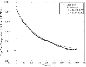
−50 0 50 100 150 200 250 300 350 400 450 −200

0 200 400 600 800 1000

Time (s)

Top Plate Temperature (

µ

K from 2.13215K)

GRT Top Fit to decay R = 14,000 K/W C = 10.34 mJ/K

Figure 3.1. Top endplate response to heat pulse.

[image:34.612.120.458.73.339.2]

In table 3.2 we show the calibration values used to computeV = aI3_{+ b}_I2_{+ R}_I_{+ d.}

Table 3.2. Heater calibrations

a b R d

HT,1 0 −1.1052 106 10192 −2.2135 10−6 HT,2 3.4857 109 −1.0018 106 10154 2.7235 10−5 HB 3.153 109 −8.0146 105 10161 1.6587 10−5

3.3

Endplate Heat Capacity

Since we are doing a high-fidelity heat capacity measurement of the liquid helium in our cell, we

need to measure the heat capacity of the empty cell in case we have to subtract it to get the true

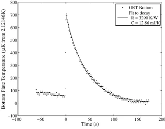
value for the helium. We measured the heat capacity of each endplate separately. We applied a 9µJ

pulse to the endplate while measuring the temperature with a GRT. We used the initial temperature

step to determine the heat capacity and then monitored the decay back to the original temperature.

The results for the cell top are shown in fig. 3.1 and those for the cell bottom in fig. 3.2.

The exponential decays were fit using the just measured end plate heat capacity and the

previ-ously measured thermal resistances. For the cell top, we needed to use a sidewall thermal resistance

(35)

combi-−100 −50 0 50 100 150 200 −100

0 100 200 300 400 500 600 700 800

Time (s)

Bottom Plate Temperature (

µ

K from 2.12146K)

[image:35.612.154.494.76.342.2]

GRT Bottom Fit to decay R = 3290 K/W C = 12.86 mJ/K

Figure 3.2. Bottom endplate response to heat pulse.

nation ofR3,4= 4300 K/W and RSidewall= 14000 K/W. The good agreement between fit and data

confirms that we have properly measured the heat capacities and thermal resistances. The final

results for the heat capacities are given in table 3.3.

Table 3.3. Heat capacities of the endplates CT 10.3 mJ/K

CB 12.9 mJ/K

3.4

Filling the Cell

While the cell bottom endplate was thermally controlled to 2.7 K, we applied 915 torr of isotopically

pure4_{He (with a}3_{He concentration of less than one part in 10}7_{) to the cell fill line and waited for}

the cell to fill. We then closed the cryo-valve by applying 580 psi of3_{He to the actuator line using}

the concentrator described in sec. 2.4.4.

We removed the remaining helium in the fill line and then pumped on the line with a leak

detector to achieve a good vacuum and therefore good thermal isolation. The leak rate settled to

approximately 10−7_{atm cm}3_/_{s. Given our 4 month cooldown, the estimated total volume of liquid}

(36)

24

safely ignored. In order to maintain a good vacuum, we attached a charcoal cryo-pump to the line,

which we periodically cleaned. During transfers, it is possible that, when the actuator pressure fell

to 420 psi, the leak rate could have increased. However, the total time that the valve was at the

reduced pressure over the lifetime of the cooldown was not more than 10 hours.

3.5

Cavitating the Bubble

Once the cell was full, we cooled it to the lambda transition. As the helium contracted, we estimate

that 0.2% of the sample was vapor. The molar volume at SVP and 2.7 K is 27.860 cm3_/_{mol, and}

at Tλ it is 27.386 cm3/mol [17]. The compressibility at 2.7 K is 1.87×10−5torr−1 [18]. Finally, at

2.7 K, SVP is 111 torr [19]. From this we compute the bubble size as

Vgas

Vliq =

27.86 cm3/mol 1−(915 torr−111 torr) 1.87×10−5_torr−1

−27.386 cm3/mol

27.386 cm3_/_mol (3.1)

= 0.002. (3.2)

We can use the cell and bubble chamber volumes computed in sec. 2.4.2, the molar volume of helium,

and the size of the bubble to compute the number of moles in our sample.

n = 0.998 V/Vm= 0.998 10.59 cm3+ 0.107 cm3/(27.386 cm3/mol)

= 0.390±0.002 mol (3.3)

Unfortunately, we could not be sure that the bubble would form inside the bubble chamber. We

cooled down to 1.8 K in order to collapse the bubble and then warmed the cell with the heater

attached to the bubble chamber to encourage the bubble to nucleate there. We carefully monitored

the temperature during this procedure, hoping to see evidence of bubble collapse or formation as

seen by others [20]. However, due to our large volume of helium and lack of thermometer on the

bubble chamber, we never saw such a signature.

We do have circumstantial evidence of when the bubble was inside the bubble chamber. On

a couple of occasions, we accidentally applied too large a heat to the cell top, causing the cell to

warm well past the lambda point. Upon cooling back to the lambda point, and investigating the

SOC state, we noticed that the SOC temperature now seemed to be dependent on the temperature

at the top of the cell. A set of data showing this effect is shown in fig. 3.3. At t = 0, the SOC

state is established in the bottom of the cell, and a small amount of superfluid still exists at the top

(as in profile A of fig. 1.1). Then, the heat added to the cell top heater is increased and the top

warms until normal fluid forms and the SOC/normal interface slowly moves down the cell. When

(37)

In fig. 3.3(b), however, we can see the SOC temperature falling as the cell top warms. Each time

normal fluid enters at the top of the cell (between 100 and 155 s and between 185 and 220 s), the

temperature recorded by the bottom thermometer drops. The midplane thermometer (not shown)

shows the same drop in temperature.

When a small bubble is at the top of the cell and the liquid helium is in the superfluid phase,

the heat flows around the bubble through the superfluid liquid, preventing any temperature or

pressure gradient in the bubble. When superflow breaks down, the top endplate warms quickly

and evaporates some of the helium which increases the pressure in the bubble. Using the SVP fit

from Donnelly [19], the 35000 nK temperature rise that we see in fig. 3.3(a) increases the pressure

in the bubble by 0.442 Pa. Given the 1.273µK/cm gradient in Tλ and the liquid helium density

of 0.14 g/cm3_{, the pressure increase causes a 41 nK drop in}_T

λ. Of course, there is a pressure and

temperature gradient across the bubble because the warm helium gas is condensing at the bottom

of the bubble which is colder. Therefore, the pressure at the bottom surface of the bubble will be

less than the full 0.442 Pa and the drop in Tλ will be less than 41 nK. We see a drop of 22 nK in

fig. 3.3(b).

On the occasions where we observed this phenomenon, we repeated the procedure of cooling

down to 1.8 K and warming with the bubble heater. We then confirmed that the SOC temperature

was once again independent of the cell top temperature and therefore assumed that the bubble was

(38)

26

0 50 100 150 200 250 300 −0.5

0 0.5 1 1.5 2 2.5 3 3.5

4x 10

4

Time (s)

Top Temperature (nK, arbitray org.)

(a) Cell top temperature as heat is added and removed.

0 50 100 150 200 250 300 −25

−20 −15 −10 −5 0 5

Time (s)

Bottom Temperature (nK, arbitray org.)

(b) Cell bottom temperature shows the effect onTλof warming and cooling the bubble at the top of the cell.

(39)

−4000 −3000 −2000 −1000 0 1000 2000 2.1747

2.1748 2.1749 2.175 2.1751 2.1752 2.1753 2.1754 2.1755 2.1756

GRT Top Temperature (K)

HRT Top (flux)

Slope: 1.8055e−07

Figure 3.4. Calibration of the top HRT to the top GRT during a ramp down of 1 mK from just below the superfluid transition.

3.6

HRT Calibration

With the entire cell just below the superfluid transition, we slowly ramped (150 nK/s) the cell

downwards in temperature about 1 mK while recording the cell top HRT and GRT. The results are

shown in fig. 3.4. We fit the top HRT flux to the top GRT temperature to get a calibration for the

cell top HRT.

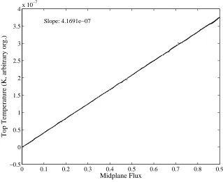
To get calibrations for the other two cell HRTs, we did a slow drift (0.1 nK/s) of about 350 nK

close to Tλ, and calibrated each of these thermometers to the cell top HRT. The results are shown

in fig. 3.5 and fig. 3.6. On a previous cooldown, we had calibrated the HRT on stage 3 near Tλ.

However, since this HRT now operates over a different temperature range, the calibration is only

approximate for the current cooldown. Each HRT does not necessarily have the same paramagnetic

material nor permanent magnets of the same strength. Therefore, the calibrations vary widely

among the HRTs. The results are summarized in table 3.4.

Table 3.4. HRT calibrations HRTT 180.6±0.9 nK/Φ0 HRTM 416.9±2.1 nK/Φ0 HRTB 81.85±0.41 nK/Φ0

(40)

28

0 0.1 0.2 0.3 0.4 0.5 0.6 0.7 0.8 0.9 −0.5

0 0.5 1 1.5 2 2.5 3 3.5

4x 10

−7

Slope: 4.1691e−07

Midplane Flux

Top Temperature (K, arbitrary org.)

Figure 3.5. Calibration of the midplane HRT to the top HRT during a drift of 350 nK.

0 0.5 1 1.5 2 2.5 3 3.5 4 4.5 5 0

0.5 1 1.5 2 2.5 3 3.5

4x 10 −7

Slope: 8.1845e−08

Bottom Flux

[image:40.612.128.447.85.346.2]

Top Temperature (K, arbitrary org.)

(41)

150 155 160 165 170 175 180 185 190 195 200 −0.3

−0.2 −0.1 0 0.1 0.2 0.3 0.4

Time (s)

Top Temperature (nK)

Noise: 0.13 nK/√Hz

Figure 3.7. Noise of the top HRT.

3.7

HRT Noise and Drift

To obtain a value for the HRT noise, we measured each HRT while the helium sample was in

the superfluid state with minimal temperature drift. The results, averaged to 1 Hz, are shown in

Figs. 3.7, 3.8, and 3.9. The standard deviation from the three data sets was used to compute the

thermometer noise given in table 3.5.

Table 3.5. HRT noise HRTT 0.13 nK/

√

Hz HRTM 0.18 nK/

√

Hz HRTB 0.11 nK/

√

Hz

In analyzing our longer data files, we matched measurements of TSOC(Q) for the same heat

flux Qthat were taken many hours apart and found we had a thermometer drift of approximately

(42)

30

150 155 160 165 170 175 180 185 190 195 200

−0.3 −0.2 −0.1 0 0.1 0.2 0.3 0.4

Time (s)

Midplane Temperature (nK)

Figure 3.8. Noise of the midplane HRT.

150 155 160 165 170 175 180 185 190 195 200 −0.25

−0.2 −0.15 −0.1 −0.05 0 0.05 0.1 0.15 0.2 0.25

Time (s)

Bottom Temperature (nK)

[image:42.612.119.456.86.352.2]

(43)

3.8

Kapitza Resistance

Well into the superfluid (20µK or so) we took a quick measurement of the regular Kapitza resistance.

This is the thermal boundary resistance that arises due to a phonon mismatch across a boundary

between two different materials. We lowered the applied heat on the top endplate by about 2µW

and increased the heat on the bottom to compensate. The helium temperature stayed roughly the

same (see sec. 3.9 for the caveat to this), but the top and bottom endplates changed temperature,

allowing us to compute Kapitza resistances across these endplates. They are presented in table 3.6.

Table 3.6. Kapitza resistances

RK,T 0.31 K/W

RK,B 0.25 K/W

There is another component to the thermal boundary resistance from the endplate into the

helium. The superfluid portion of the helium is suppressed near a boundary. Near Tλ, the region

over which the superfluid is suppressed gets large and causes a significant increase in the thermal

boundary resistance. This has been measured previously in “heat-from-below” configurations [21]

and we attempted to measure this singular component of the Kapitza resistance in our

“heat-from-above” configuration. Unfortunately, we measured a heat-flux-dependent resistance. This is

caused by having helium in the gap between the endplate and the sidewall [14, 15]. As discussed in

sec. 2.4.2, we suspected this might be the case during cell construction. Also, the fact that we see a

lower regular Kapitza resistance for the bottom endplate, despite a surface preparation identical to

the top, suggests there may be a sidewall gap.2

3.9

Heater Response Times

Our heat capacity measurements, which will be described in the next chapter, are very sensitive to

any lag time between applying a voltage to the current source and heat being deposited into the

experiment. At one moment in the experiment, the power dissipated in one heater is decreased by

the same amount as the increase in another cell heater. If there is no significant lag in the response,

or if the lag is equal for both heaters, then no energy will be gained or lost by the helium as this

switch between the heaters occurs.

3.9.1

The Problem

By measuring the voltage across two wires of the 4-wire heater when a pulse of current was applied,

we found that any lag was less than one millisecond. This means there are no problems with the

(44)

32

−400 −200 0 200 400 600 800 1000 1200 1400

−40 −35 −30 −25 −20 −15 −10 −5 0

Time (ms)

Temperature (nK, arbitrary org.)

Figure 3.10. Temperature response of the top endplate HRT caused by swapping heat from one heater to another heater with a different time constant.

DAC or current source. However, with the sample entirely in the superfluid, swapping heat from

HT,2 to HB resulted in a small but noticeable change in the helium temperature. The small cell

temperature drift was the same before and after the swap.

To confirm that this effect was due to a time lag problem and not some exotic properties of the

helium, we repeated the same experiment, except we swapped heat from HT,2to HT,1, heaters that

are on the same endplate. In fig. 3.10, we see the temperature response of HRTT to the swap at

t= 0 with very little data averaging. Obviously, the heater that was reduced responded faster than

the heater that was increased. The output is complicated by both the time constant of the copper

endplate relaxing to the thermal bath of the helium sample and the time constant of the HRT coming

into equilibrium with the endplate. The end result, only seen with more data averaging for lower

noise, is that the helium cooled about 1 nK. When we reverse the swap, the response is identical,

but in the reverse direction. Since we are swapping between two heaters on the same endplate, there

is no change in heat flux through the sample, so no helium properties could cause this effect.

We hypothesize that this time constant is caused by the heaters being poorly attached to their

locations resulting in an appreciable thermal contact resistance. When a voltage is applied, the

heater responds immediately. However, the heater, with its heat capacity and thermal resistance

(45)

resistance, so the time constant is different for each one. A further complication is that this time

constant appears to change with heat flux. This could be due to either the heater’s heat capacity

or thermal contact resistances changing as the heater changes temperature.

3.9.2

The Solution

Our solution was to calibrate and quantify the size of this error by performing the same experiment

where we first saw the effect. We cool well below the superfluid transition and swap the heat from

the top heater to the bottom and observe the temperature change of the helium. Using the heat

capacity of the helium, it is possible to extract how much energy was lost or gained in the swap. We

need to perform this experiment with the same pair of heaters for the same heat fluxes that we use

in our heat capacity measurements for the calibrations to be helpful.

To improve the calibrations, the actual procedure worked as follows. For each pair of heat flux

values, we swapped back and forth while intentionally delaying the change of the faster heater by a

time, τ. We started with small delays and then gradually increased their length. We then plotted

the temperature change of the helium vs. the delay. Fig. 3.11 is an example of this. We fit the

results to a line. The zero crossing of this line tells us how much time delay is necessary so that no

energy is gained or lost. If the faster heater was changed by an amount of heatA∆Q, whereA is

the cell cross-sectional area, then the energy ∆E gained for no delay is ∆E=τ A∆Q. We did not

perform this experiment for every pair of heat flux values, but instead changed the heat flux through

the cell from 0 to 1 µW/cm2_{, from 1 to 2} _µ_W_/_cm2_{, from 2 to 3}_µ_W_/_cm2_{, and so on. We then fit}

the resulting curve to a parabola (or a line if there were fewer than four points) which allowed us to

scale ∆E for any heat flux swap.

3.10

Heat Leaks

Unfortunately, in the design and construction of the experimental cell, we made a miscalculation

of the size and arrangement of the copper foils that are placed on the mounting plate. One set

of foils was intended to conduct away the heat flux, and the other set of foils was to maintain a

heat sinking location close in temperature to the cell bottom endplate. Either through high contact

resistance, higher than expected conductivity of titanium, or some other unexpected reason, the

temperature of the heat-sinking foils was significantly different from the cell bottom endplate. This

gave us relatively large heat leaks (a few nanowatts) through the HRTs and their Vespel mounts

(46)

34

0 5 10 15 20 25 30 35 40 45 50

−2 −1 0 1 2 3 4 5

Time (ms)

Helium Temperature Change (nK)

(47)

10 15 20 25 30 35 40 2.1715

2.172 2.1725 2.173 2.1735 2.174 2.1745 2.175

Bottom Plate Servo Power (µW)

Bottom GRT Temperature (k)

Figure 3.12. Dependence of GRT bottom on heat flux.

3.10.1

The Problem

To quantify the effect, we performed a simple experiment. We controlled the cell bottom HRT with

a servo to a set flux value and then ramped the stage 3 temperature up and down. Since the heat

flux extracted from the cell is determined by the temperature difference between the cell and stage 3,

the servo power went down and up to compensate. In fig. 3.12, we plot the cell bottom GRT versus

the servo power. Since the cell bottom GRT is mounted on the heat sinking foil and not on the cell

bottom endplate itself, we can see the magnitude of the problem. Despite the cell bottom endplate

remaining constant in temperature, the heat-sinking foil is changing in temperature by over 1 mK.

Therefore the foils which we had hoped would be at the cell bottom temperature are actually offset

in temperature due to a resistance of over 100 K/W.

With just a couple of exceptions, all the experiments we performed in this cooldown kept the

temperature difference between the cell and stage 3 nearly constant. When that is the case, the heat

leaks will be constant during the experiment. The first exception is HRT calibration, where we were

careful and used the top HRT and top GRT, which are immune from this type of heat leak. The

second exception is the experiments described in this section.

In a typical configuration, the total power flowing from the cell to stage 3 was 20µW. Given an

(48)

36

A heat leak causes two problems. The first is the leak could reduce or distort the heat flux.

Our experiments are not particularly sensitive to these effects since our heat fluxes are relatively

large. Only at our smallest heat fluxes, 30 nW/cm2_{, will leaks on the order of 1 nW be noticeable.}

The second effect is caused by the heat leak flowing across a thermal resistance through the HRT

and out the HRT support. This causes the HRT to read a temperature that is offset from the

true temperature. As long as the thermal resistance remains the same, however, the offset will be

constant. Therefore, the heat leak through HRTT and HRTB can be ignored. However, the heat

leak through the foil HRT flows across a helium/copper boundary which has a Kapitza resistance.

The singular component of the Kapitza resistance is strongly dependent on the helium temperature

close toTλand therefore HRTMhas a variable temperature error that prevents it from reading the true helium sample temperature.

3.10.2

The Solution

Luckily, we mounted a heater on the copper bar connecting HRTMwith the penetrating sidewall foil.

Therefore, if we could properly compute how large the heat leak was, we could apply exactly the

Experiments on the Self Organized Critical State of 4He

Andrew Rosenberg Chatto

Abstract

Contents

List of Tables

Chapter 1

The SOC State

The SOC Heat Capacity

0

Heat Capacity (J/mol K)

The SOC State Wave

Summary

Chapter 2

Cryogenic System

Thermometry

Auxiliary Stages

Cell Stage

Cell Construction

Fill Line and Bubble Chamber

Cryo-Valve and

HRT Mounting

GRT Mounting

Heaters

Data Acquisition and Experiment Control

Data Acquisition and Control

Computer Inputs and Outputs

Computer Software

Chapter 3

Heater Calibrations

Endplate Heat Capacity

Filling the Cell

Cavitating the Bubble

HRT Calibration

Time (s)

Time (s)

Heater Response Times

The Problem

The Solution

Heat Leaks

The Problem

The Solution