(will be inserted by the editor)
The TPS Direct Transport: a new method for transporting
deformations in the Size-and-shape Space.
Valerio Varano1 · Stefano Gabriele1 · Luciano Teresi2 · Ian Dryden3 ·
Paolo E. Puddu4 · Concetta Torromeo4 · Paolo Piras4,5
Received: date / Accepted: date
Abstract Modern shape analysis allows the fine com-parison of shape changes occurring between different objects. Very often the classic machineries of Gener-alized Procrustes Analysis and Principal Component Analysis are used in order to contrast the shape change occurring among configurations represented by homol-ogous landmarks. However, if size and shape data are structured in different groups thus constituting differ-ent morphological trajectories, a data cdiffer-entering is needed if one wants to compare solely the deformation rep-resenting the trajectories. To do that, inter-individual variation must be filtered out. This maneuver is rarely applied in studies using simulated or real data. A geo-metrical procedure named Parallel Transport, that can be based on various connection types, is necessary to perform such kind of data centering. Usually, the Levi Civita connection is used for interpolation of curves in a Riemannian space. It can also be used to transport a deformation. We demonstrate that this procedure does not preserve some important characters of the deforma-tion, even in the affine case. We propose a novel pro-cedure called ‘TPS Direct Transport’ which is able to perfectly transport deformation in the affine case and to better approximate non affine deformation in compar-ison to existing tools. We recommend to center shape
Valerio Varano
E-mail: [email protected]
1 Department of Architecture, Roma Tre University, Roma, Italy.
2Department of Mathematics & Physics, Roma Tre Univer-sity, Roma, Italy.
3School of Mathematical Sciences, University of Nottingham, Nottingham, UK.
4 Department of Cardiovascular, Respiratory, Nephrological and Geriatric Sciences, Sapienza University, Rome, Italy. 5 Department of Structural Engineering and Geotechnics, Sapienza University, Roma, Italy.
data using the methods described here when the dif-ferences in deformation rather than in shape are under study.
Keywords Geometric Morphometrics·Shape Analy-sis·Inter-individual difference·Riemannian Manifold·
Deformation cycle· Parallel Transport · Trajectory Analysis·Thin Plate Spline.
1 Introduction 1.1 State of the Art
Shape theory became central in many fields from com-puter vision to biological and medical applications; ac-cording to [41], it can be split in at least two prin-cipal frameworks: i) shape optimization, that is, the search for the best shape according to a criterion; ex-amples include image segmentation and object track-ing; and ii) shape analysis, consisting in the study of families of shapes for statistics, (automatic) cataloging, probabilistic modeling, etc. The former is more used in computer vision, and relies on continuum formula-tions (diffeomorphisms, active contours, parametrized surfaces etc.); the latter is more used in biological appli-cations, and is based on the discrete sampling of shapes by means of homologous landmarks, which are carefully selected according to anatomical features. Recently, the field of computational anatomy translated the contin-uum approaches in medicine and biology.
embodied in two notions: i) the metric, measuring the distance between points (that is, shapes); ii) the con-nection, yielding the geodesic connecting two points. It is worth noting that a connection has to be compati-ble with the metric, and can be built upon a Parallel Transport (PT), a rule for transporting vectors along geodesics.
Moreover, a PT is compatible with the metric when it does not change the length of vectors and the an-gles between them. For a given a metric, there exists a unique PT compatible with it, and having vanishing torsion: the Levi Civita (LC) PT. (The torsion of the connection is a slightly technical notion that we will discuss in the following).
According to [48], PT can be used in Shape theory for many purposes, such as defining geodesics between shapes, transporting a deformation from one shape to another, creating random sampling for statistical shape models. In the case of shapes sampled by homologous landmarks, the LC connection is often used to define the geodesic between two shapes, and to transport de-formations [19]. However, it can be proved [47] that this approach does not preserve some important fea-tures of the deformation. [44] discusses the problem of comparing the deformations occurring between pairs of shapes and groups of shapes (in particular they for-malize the concept of correspondence). The LV PT in the Kendall’s Shape Space has been used in the past for 2D configurations [14, 18] with explicit formulas; re-cently, [47] proposed a new 2D explicit formula for LC PT in the Kendall’s Size-and-Shape Space.
Many efforts have been done in recent years in order to unify shape metrics with deformation metrics, see [7,27,28,34,48], whose complete review is far beyond the scope of the present paper. In particular, new metrics have been proposed together with the corresponding connections.
A morphometric approach based on diffeomorphisms (namely ’diffeomorphometry’) has been recently patented for surfaces (not necessarily identified by homologous landmarks) acquired by CT scan [29]. For example, [42](fig.1) proposed a strategy that is similar in aim to the one presented here. [28, 31] revise the theory be-hind this attractive approach that traces back to [46] and [45]. It stems from the computation of geodesics by means of the Large Diffeomorphic Deformation Metric Mapping (LDDMM) approach for which we refer the reader to [13, 28] and references therein.
In classic Geometric Morphometrics, [2], [9], the de-formation between two shapes is evaluated using the Thin Plate Spline (TPS) method, that is a function that minimizes the bending energy [1].
TPS, however, is a non-bijective interpolating func-tion, and has no inherent restrictions to prevent folding, even if some efforts have been made to tackle this is-sue [11]. Moreover, given two shapes, a target and a source, TPS is ‘source dependent’ and swapping tar-get with source yields a different deformation path. In Geometric Morphometrics it is a consolidated prac-tice to decompose the whole deformation in affine and non affine components. The same is done in other con-texts such as in the “deformotion” approach proposed by [49]. [41] proposed a tri-partite decomposition of the deformation (translation, scaling, all the rest) in the framework of the active contour approach, while [32] did the same in the context of LDDMM, in order to manage the non scale-invariance of LDDMM transfor-mations. None of the aforementioned methods yield a PT compatible with the affine/non affine decomposi-tion and do not consider the PT of the affine part of the deformation toward a target shape. When a PT is built upon the above mentioned methods, the LC con-nection is the main tool for transporting deformation. This PT, based on the LC connection, is dependent from the path, and some efforts have been done to pro-pose path-independent strategies [12, 25].
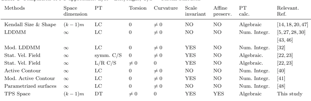
Table 1 (far to be exhaustive) summarizes the prin-cipal features of the most common approaches proposed in the last years.
In the present paper we propose a PT that has two properties: i) it is independent from the path; ii) it is compatible with the affine/non affine decomposition. We couple this strategy with a data-centering aimed at eliminating inter-individual differences and with a trajectory analysis aimed at recovering the original de-formational series, once shapes have been transported. In the present article we focus on the landmark-based shape theory, i.e. Geometric Morphometrics.
ordina-Table 1 Comparison of PT approaches. L/R= Left/Right; C/S = Cartan-Schouten
Methods Space PT Torsion Curvature Scale Affine PT Relevant.
dimension invariant preserv. calc. Ref.
Kendall Size & Shape (k−1)m LC 0 6= 0 NO NO Algebraic [14, 18, 20, 47]
[image:3.595.41.556.99.267.2]LDDMM ∞ LC 0 6= 0 NO NO Num. Integr. [5, 27, 28, 30]
[43, 46]
Mod. LDDMM ∞ LC 0 6= 0 YES NO Num. Integr. [32]
Stat. Vel. Field ∞ symm. C/S 0 6= 0 YES NO Algebraic. [22, 23]
Stat. Vel. Field ∞ L/R C/S 6= 0 0 YES NO Algebraic. [22, 23]
Active Contour ∞ LC 0 6= 0 NO NO Num. Integr. [40]
Mod. Active Contour ∞ LC 0 6= 0 YES NO Num. Integr. [41]
Parametrized surfaces ∞ LC 0 6= 0 NO NO Num. Integr. [48]
TPS Space (k−1)m DT 6= 0 0 YES YES Algebraic This study
tion methods, such as Principal Component Analysis (PCA) for further analysis. If one is interested also in the size variation, the appropriate space is the Size-and-shape Space, where only translations and rotations are eliminated by obtaining the so calledforms.
1.2 The contributions of the present paper
In this paper we deal withtrajectory of forms, defined as ordered sequence of forms, and we investigate the differences among trajectories, irrespective of the dif-ferences of the forms they contain.
We show that shape analysis of trajectories should be performed only after a proper representation of each shape of a trajectory has been obtained, and before ap-plying ordination methods. In fact, studying the form of a trajectory means studying how the deformation changes along each path irrespectively of the actual form to which these deformations apply. The indepen-dence of the deformation from the form to which it is applied is critical: it implies that any form variation between individuals at the beginning of each trajecto-ries must be completely filtered out. Often, in statis-tics, inter-group differences are eliminated by apply-ing a group-mean centerapply-ing, optionally followed by the Grand Mean addition.
A problem arises if the data are shape or form data. Very frequently the LC connection on the Shape Space is used to compute the geodesics between two shapes [18, 20]. Sometimes it is also used to transport a mation along this geodesic, in order to apply a defor-mation from one shape to the another shape [14,19,48], where the torsion of the connection is zero. Formally, this procedure could be applied in order to center data in the Shape Space, but it is revealed to be inadequate in some cases because it does not preserve the physical meaning of the deformation during the path.
Many efforts have been done in recent years in or-der to unify shape metrics with deformation metrics [4,21,27,30,32,34,44,48]; in general, independently from the used description (landmarks based, parametric, dif-feomorphism based), new metrics have been proposed together with the corresponding induced LC connec-tions. Because LC connection can be written in terms of the metric, PTs are determined uniquely by metric issues.
Here we show how a new connection that we call ‘TPS Connection’ allows, by means of a ‘TPS DT’, to compare different form trajectories by performing a data centering which maintains the nature of the de-formations. In particular the DT is compatible with the decomposition of the deformation to affine and non affine components. The adjective ‘Direct’ means that PT does not depend on the path, then the Riemannian curvature of the connection is zero. Moreover the DT is compatible with an introduced new Riemannian metric (TPS metric) but is different from the LC transport, as the torsion of the connection is different from zero. Despite all the technicalities related to the landmarks based description, the idea to give up the symmetry of the connection to obtain a connection flat and com-patible with a significant decomposition of the tangent spaces could be exported to other contexts.
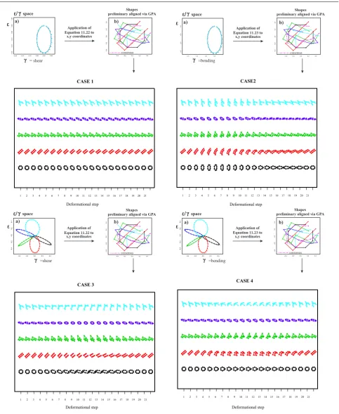
We used simulated datasets and an a priori known set of affine and non affine parametrized deformations in order to build properly pre-processed form trajec-tories to be used in standard ordination methods such as PCA. As far as we know there are few or no con-tributions aimed at performing such ”reverse engineer-ing” strategy. This allows to control the properties of final result and to perform specific performance anal-yses allowing to appreciate if the original deformation trajectories are properly transported toward the target shape. In addition, we illustrate the methodology with an application in cardiology, which motivates the work. To summarize, the main contributions of the present work are:
– Trajectory Analysis via Data Centering in Riemannian Manifold
While PCA on centered data is used in many pa-pers (e.g. the concept of atlas in functional anatomy [5, 28]), as well as trajectory analysis via the use of different kinds of PT ( [10, 24, 33, 36, 50, 51]). How-ever, the idea of performing a shape analysis on the shapes of trajectorythemselves, evaluated at physi-ological homologous times in order to assess the bi-ological function has been introduced the first time in [35] and formalized in [47]. In that papers, has been widely shown as this procedure leads to better disease classification.
– TPS Metric
In both LDDMM and active contour frameworks, it has been proposed a decomposition of the de-formation (together with a compatible metric), [32] and [41]; this decomposition only uncouples scaling from the rest of the deformation, without distin-guishing between global affine deformations (size, aspect ratio and shear), and local ones (non affine component). Such a recognition of the difference be-tween these two features of a deformation is instead present in the original formulation of TPS by Book-stein, but the decomposition is not accompanied by a Riemannian metric, being the bending energy only a singular metric which vanishes on all the affine de-formations.
– TPS Direct Transport
The main features of the DT are: 1) it is compat-ible with the above mentioned TPS metric, 2) it is compatible with the given decomposition, 3) it is path independent, i.e. it induces a flat space. In particular the first feature means that the DT is an isometry with respect to the TPS metric. The sec-ond feature means that the transported vector of the original affine component coincides with the affine component of the transported vector and the same holds for the non affine component. The third
fea-ture makes the whole procedure very simple from a conceptual point of view and computationally very cheap as it does not require any integration proce-dure: no calculation of the geodesics, no calculation of the PT along geodesics, only a closed form ex-pression.
Moreover, the peculiarity of the DT, with re-spect to the most common PT used in shape analy-sis is the way it is built. It is not defined in terms of a given covariant derivative (e.g. in terms of Christof-fel symbols), by integrating ODEs. It is directly for-mulated in terms of a givenrule, by checking that it respects some abstract requirements characterizing any PT that represents a connection on a mani-fold [8]. This procedure is common in classical dif-ferential geometry. In fact, as stated above, the DT is a type of Weitzenbock connection.
– Reverse Engineering Experiments
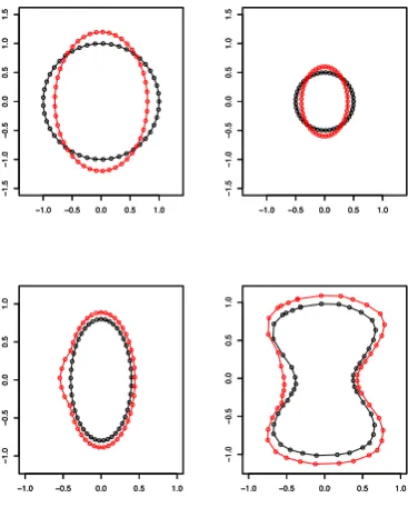
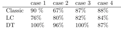
The performance of PT here proposed, together with the whole procedure of data centering, is assessed by means of shape analysis on ad hoc shape data: we generate sequences of shapes by using parametrized deformation; our goal is to recover the values of the parameters used to generate the data set. This ap-proach is rarely found in related literature.
All the following examples and analyses were per-formed in R using the package ‘deformetrics’ avail-able on github. It can be installed using the in-stall github() function in ‘devtools’ R package by typing the following command line:
install github(‘deformetrics/deformetrics’,local=FALSE).
2 The geometrical structure of the shape space A bodyB is an open subset of the m-dimensional Eu-clidean ambient space Em; the positions x ∈ Em of k points, called landmarks, define aconfiguration of the body, which can be represented as a k×m matrix
X = (x1, . . . , xk)T; we denote with Cmk the
Configura-tion Space, that is, the set of all possible configurations. The Shape Space Σk
m can be defined as the quo-tient ofCk
m under the action of the groupS(m) of the Euclidean similarity transformations inEm. S(m) can be decomposed in three subgroups: translationsT(m); rotations SO(m); homothety or dilatation H(m). The Shape Space can be conveniently generated by remov-ing similarity transformations one by one; the first step is to remove location, translating each configuration in such a way that the centroid lies on the originoof the Euclidean space. This brings us to the Centered Con-figuration Space CCk
The successive filtering can be done by removing rotations–thus obtaining theSize-and-Shape SpaceSΣk m; eventually, by removing size, we obtain the Shape Space as Σk
m = SΣkm/H(m) [9]. To summarize, we consider the following spaces:
Cmk ,Configuration Space;
CCmk ,Centered Configuration Space;
SΣmk =CCmk/SO(m),Size-and-Shape Space;
Σk
m=SΣmk/H(m),Shape Space;
For each of the aforementioned spaces a suitable parametrization is needed. Here the Centered Config-uration Space CCk
m is parametrized in two complemen-tary ways:centered landmarksorHelmertized landmarks. The first is a redundant parametrization while the sec-ond is a strict one. Both the parametrizations are ob-tained by pre-multiplying the coordinates matrixX by a suitable matrix.
We define thecentered configurationXCas thek×m matrix:
XC=CX
whereC=Ik−k11k1Tk, Ik is thek×kidentity matrix and 1k is a k×1 column of ones.
We define the Helmertized landmarks XH as the (k−1)×mmatrix:
XH=HX
whereH is the so called Helmert sub-matrix. Thej−th
row of the Helmert sub-matrixH is given by
(hj, ..., hj,−jhj,0, ...,0), hj=−(j(j+ 1))−1/2
and so the j−th row consists ofhj repeated j times, followed byjhjand thenk−j−1 zeros,j= 1, ..., k−1. One can switch from one parametrization to the other by using the properties:
HTH =C ,
and then
XC=HTXH, XH=HXC.
Theform (otherwise calledsize-and-shape) of a config-uration X is the equivalence class [X]S ∈ SΣmk repre-sented by:
[X]S ={XCQ:Q∈SOm}.
Finally, theshape of a configurationX is the equiv-alence class [X]∈ Σk
m defined as:
[X] = [X]S/||XC||
where||XC||= (trace(XCTXC) )1/2is the Centroid Size (CS) ofXC, the most used measure of size in Geometric Morphometrics. We call anicona particular member of the shape set [X] which is taken as being representative of the shape. To summarize, we consider the following elements:
Configuration: X ∈ Ck
m;
Centered Configuration: XC,orXH ∈ CCmk ; Form or Size-and-Shape: [X]S ∈ SΣmk ;
Shape: [X]∈Σk
m.
Let us note that the procedure described above de-fines implicitly an atlas for the shape space, which in-herits a manifold structure. Actually, the Shape Space by Kendall has a richer geometric structure, being en-dowed with: i) a Riemannian structure, defined by a metric (gΣ) on the tangent bundle; ii) a distance (dΣ) on the manifold; iii) a connection, defined by a covariant derivative (∇Σ) on the tangent bundle. It is important to stress that, in principle, these definitions are inde-pendent of each other, and the richness of the resulting geometric structure is overshadowed by both the ele-gance of the Kendall’s construction, and by the tacit identification CCk
m ≡ R(k−1)m ≡ E(k−1)m of the cen-tered configuration space CCk
m with the (k−1)×m Euclidean SpaceE(k−1)m; in particular, it is assumed that this identification holds for each level of the geo-metrical structure. The meaning and the consequences of this assumption will be discussed below.
Once accepted that the entire geometrical structure ofE(k−1)m is inherited by CCk
m, one observes that the regular part of the shape space Σmk is built by a se-quence of Riemannian isometric maps: a quotient map
π(submersion) followed by an hortogonal projection$
(immersion):
CCmk ≡ E(k−1)m quotientπ
−−−−−−→
submersion SΣ
k m
orthogonal projection$
−−−−−−−−−−−−−→
immersion Σ
k m.
This sequence induces isometrically all the geometric structure from the configuration spaceCk
mto the shape spaceΣk
m; details can be found in [16], [20].
Here, it is useful to recall that in the Euclidean space
Ek m, the tangent spaces at any point can be identi-fied with a global vector spaceRk m, i.e. the translation
space ofEk m. Thus, to each pair of points (Y, X) there corresponds a vectorV =Y −X ∈ Rk m. Vectors be-longing toRk mare calleddeformation vectors; the
Eu-clidean metric tensor corresponding to the dot product
U·V = trace(UTV) is then naturally used to define an Euclidean distance:
d(Y, X) =||Y −X||=p(Y −X)·(Y −X).
Euclidean space structure by recalling that the connec-tion onEk m, in particular the LC connection, gives rise to parallel transports that are simple translations.
The induced distance on the size-and-shape space
SΣk
mis:
dS([Y]S,[X]S) = inf
Q∈SO(m)d(Y Q, X) (2.1)
= inf
Q∈SO(m)||Y Q−X||.
This definition allows us to give a procedure to align a configuration Y onto a configuration X. In particular thealigned configuration Yˆ is obtained by means of an optimal rotation Qˆ minimizing the Euclidean distance
||Y Q−X||.
ˆ
Y =YQ ,ˆ Qˆ = argminQ∈SO(m)||Y Q−X||.
It is possible to prove that ˆQ is the rotational com-ponent coming from a polar decomposition of YTX (see [9]). That is, YTX = ˆQ U with U ∈ Sym(
Rm m)
and ˆQ∈SO(m). It follows,
ˆ
QTYTX = (YQˆ)TX= ˆYTX=U .
As a consequence, we can say that two configurations ˆ
Y , X are optimally aligned if and only if the matrix
ˆ
YTX is symmetric, i.e ˆYTX∈Sym(
Rm m). This
pair-wise alignment is called Ordinary Procrustes Analysis (OPA) without scaling. When one deals with several configurations Xi a technique called Generalized Pro-crustes Analysis (GPA), allows, by means of an itera-tive algorithm, to define an average configurationXGM, called the Grand Mean (GM), and, simultaneusy, to align everyXitoXGM. In other words, at the end of a GPA, one obtains a set of configurations ˆXi, such that for eachi, ˆXT
i XGM ∈Sym(Rm m)
Each tangent spaceTX(CCmk) at the centered con-figuration XC ∈ CCmk can be identified with the global vector space R(k−1)m; moreover, with respect to the
quotient mapπ: CCk
m → SΣmk,TX(CCmk) splits into a vertical and a horizontal subspace:
TX(CCmk) =VX⊕ HX,
characterized as follows:
VX ={V ∈ TX(CCk m) :V =XW ,withW =−WT},
HX={V ∈ TX(CCk m) : withVTX = (VTX)T},
In practice, a vertical vector at X is an infinitesimal rotation of the configurationX, while a horizontal vec-tor is a vecvec-tor that, added toX, yields a configuration
Y =X+V aligned withX. Conversely, given a config-urationY aligned withX, their difference is horizontal.
The key feature of the horizontal subspace HX is that it is isometric toT[X]S(SΣmk), the tangent space of
SΣk
mat the form [X]S. This feature allows us to repre-sent vectors inT[X]S(SΣmk) through their corresponding vectors inHX, which are easier to handle.
3 Deformation maps and Form trajectories One basic notion that will be crucial in the following is that of adeformation map, a smooth, interpolant map
Φ : Em → Em. Given a pair of configurations X, Y ∈
Ck
m, we shall write
Y =Φ(X)
to say thatY is a deformation ofX, that is
yi=Φ(xi), ∀xi∈X , yi∈Y .
Here X is the source and Y is the target. Note that the deformation acts on the whole space Em, rather than just on a set of landmarks. A bijective deforma-tionΦ is a diffeomorphism fromEm to itself. Further-more, note that the deformation is a notion pertaining to the Configuration Space rather than to the Shape Space or Size-and-Shape Space. A family of deforma-tionsΦt:Em→ Em, smoothly parametrised by a scalar
t, is called a motion. Given a motionΦt, we define the discrete trajectory of the configurationXunder the ac-tion ofΦt as the sequence:
TΦ(X) = (Xt1, . . . , Xtn), withXti=Φti(X).
We shall tackle two main examples:
1. Different motions of the same body: given different motions Φjt, and a single configuration X, we can generate many different discrete trajectories:
TΦj(X) = (Xtj
1, . . . , X
j
tn), withX j ti =Φ
j ti(X) ;
2. Same motion of different bodies: given a motionΦt and different configurations X`, we generate many different discrete trajectories:
TΦ(X`) = (Xt`1, . . . , X
`
tn), withXti` =Φti(X`).
Please, note that the apex inXtji orX `
ti can refer both to a motionΦjt, as in the first item, or to a configuration
X`, as in the second one.
The same notion of discrete trajectory applies also to a sequence of forms; thus, we define the trajectory of the form [X]S under the action ofΦt as the sequence:
Our goal is the development of a procedure to compare forms’ discrete trajectories, and be able to discriminate between intra- and inter-form variations.
If the displacements between the forms of a discrete trajectory are small enough, they can be considered as vectors belonging to a same tangent space of SΣk
m; in this case form differences can be efficiently assessed by ordination analyses such as PCA performed on the co-variance matrix. The problem arises when two or more forms’ discrete trajectories span different and distant neighborhoods of the Size-and-Shape Space. In such a case, even if the deformations within each discrete trajectory are small, they cannot be compared: defor-mation vectors belong to very different tangent spaces. In differential geometry the tool for comparing vec-tors on different tangent spaces is Parallel Transport (PT) [8, 26, 39].
4 Parallel Transports and Riemannian Connections
The PT on a manifold is related to the connection de-fined on its tangent bundle. To be more precise, accord-ing to [8], we begin by specifyaccord-ing therule that any PT
τb,a along a path fromatob has to fulfill:
τb,a:TaM →TbM,is linear, and non-singular.
Va 7→Vb;
moreover, for any pointcon the path
τb,c◦τc,a =τb,a (4.2)
It follows from this that τa,a is the identity on TaM, andτa,b= (τb,a)−1.
Aparallel vector field is a vector field generated by parallel transporting a given vector along a path; thus,
W is a parallel field if Wb = τb,a(Wa) for each b and someaon the path. A connection is compatible with a metricgif the PT is an isometry, that is
ga(Va, Wa) =gb(τb,a(Va), τb,a(Wa)) (4.3)
for each pair of vectorVa, Wa, see [17].
Usually, a PT is defined by means of a covariant derivative ∇ along a curve γ. A vector field V is said to be parallel alongγif:
∇γ˙V = 0. (4.4)
As shown in [39], the PT is usually defined in terms of the covariant derivative∇, but one can also reverse the process: assume a parallel transport τ, and define the covariant derivative by a limit:
∇VpU = lim h→0
τh,0−1Uγ(h)−Uγ(0)
h (4.5)
Thetorsionof the connection∇is the tensor field:
∇VW− ∇WV −[V, W],
with [·,·] the Lie bracket. A connection is called sym-metric when the torsion is null, for allV, W. A funda-mental result of Riemannian Geometry is the existence of a unique symmetric connection compatible with the metric g, named the LC connection. The uniqueness of the LC connection allows us to transfer easily a con-nection from a Riemannian manifold to another one via isometric maps.
Since the work of [16], the LC connections on the Shape SpaceΣk
mand on the Size-and-Shape SpaceSΣkm have been widely studied. As outlined in the previous Section, the regular part of the Shape Space can be de-fined by means of a sequence of Riemannian immersions and submersions starting from the Centered Configura-tion SpaceCCk
m, so that the LC connection on the Shape Space can be isometrically inherited from that onCCk
m:
Connection onCCmk −−−−−−−→isometric
inheritance Connection onΣ k m.
Form= 2, PT has an explicit representation, while for
m = 3 PT can be evaluated by integrating the ordi-nary differential system (4.4). In both cases, the pro-cedure has been used to interpolate curves on Shape Space [20], [18]. On the other hand, in [14] and [48] the LC parallel transport has been used to transfer a de-formation from a shape to a different one. In [47] an explicit representation form = 2 has been introduced also for the Size-and-Shape Space, and used to compare form-discrete trajectories. In order to evaluate the util-ity of such a procedure, we need to better explain how the deformation can be defined and described.
5 Describing Deformations: the Centered Thin Plate Spline
In the previous sections we introduced two different no-tions of deformation: the deformation vector VX, and the deformation map Φ. Both are meant to transform a given configurationX onto a deformed configuration
Y: we haveY =X+VX or, alternatively,Y =Φ(X). The differences between these two notions are:
– VX represents the displacements of the landmarks, whileΦis a map defined on the whole space. – Given two close configurationsX andY, the
defor-mation vector from X to Y is unique, while there exist infinitely many mapsΦsuch thatΦ(X) =Y.
Thin Plate Spline (TPS), introduced in [1] and devel-oped in successive papers as [3, 37]. The major draw-back of the TPS is that it cannot prevent folding and cannot guaranty a diffeomorphism. For this reason it is not the mostly used regularization kernels in Computer Vision. Nevertheless it is the most used in Geometric Morphometrics, were the considered deformations are usually not so large to induce appreciable foldings. As stated above here we are considering the deformation occurring, within a single trajectory, between near con-figurations, then we will consider TPS as an acceptable representation.
The TPS representation of the deformation is often used due to the following advantages:
– The TPS interpolation has an explicit representa-tion
– it decomposes the deformation into a globalaffine transformationand a set oflocal deformationswhich highlight changes at progressively smaller scales. – it is based on the minimization of a cost-function,
called thebending energy,
– the bending energy gauges the non-affine part of the deformation as a pseudo-distance between configu-rations.
The TPS representation allows us to obtain a very mean-ingful analysis of the deformation. On the other hand there are some drawbacks in the original formulation:
– The TPS is defined in the Configuration Space rather than in the Centered Configuration Space. This in-troduces an annoying term which represents a trans-lation, even when two centered configurations are compared.
– The bending energy is a pseudo-distance, in fact it vanishes in the affine part of the deformation, so it cannot gauge the distance between two configura-tion related by a linear transformaconfigura-tion (for example a simple shear).
– The bending energy is a pseudo-distance because it is not symmetric: the bending energy in deforming
X ontoY is different from the one in deformingY
ontoX.
– The affine and non affine components, as coming from the TPS analysis, are not orthogonal in the Euclidean metric.
By following the notation of [9] we summarize the con-struction of the TPS, and we refer to [1, 9] for fur-ther details. In the Euclidean space Em, the m-tuple of interpolating TPS is a functionΨ represented by the triple (c, A, W), where: c ∈ Em is a point represented by (m×1) matrix;Ais a linear transformation ofEm, represented by a (m×m) matrix;W is a (k×m) matrix.
Given a pointx∈ Em, and a configurationX ∈ Ck m, we have
y=Ψ(x) =c+Ax+WTs(x), (5.6)
where s(x) = (σ(x−x1), ..., σ(x−xk))T a is (k×1) matrix, xi ∈ X is the position of the i-th landmark, and
σ(h) =
||h||2log(||h||) if||h||>0;
0 if||h||= 0. form= 2
σ(h) =
−||h||if||h||>0;
0 if||h||= 0. form= 3
Given a source configuration X, and a target configu-ration Y, we can apply equation (5.6) landmark-wise, yielding to
Y = 1kcT+XAT+SW , withSij =σ(xi−xj). (5.7)
There are 2kinterpolation constraints in equation (5.7), and we introducem×(m+ 1) more constraints on W
in order to uncouple the affine and non affine parts:
1TkW = 0, XTW = 0. (5.8)
For a given pair (X, Y) there exists a unique set of
m(1 +m+k) =m+m2+mkparameters for the triplet
(c, A, W) that solve the problem (5.7), constrained with
(5.8); the explicit solution can be found in the refer-ences.
Now we introduce some small changes to the original procedure in order to calculate everything directly in the Centered Configuration SpaceCCk
m. By multiplying (5.7) by C, and exploiting the following properties of the operatorC:
C=HTH , C1
kcT = 0, C W =W , (the last equation is a consequence of the constraint (5.8)) we can write
YH =XHAT +SHWH,
withYH =HY,XH =HX, andWH =HW (k−1)×m matrices, and SH = HSHT a (k−1)×(k−1) ma-trix. Everything is expresses in Helmertized coordinates that, as previously noted, is a strict parametrization of
CCk
m. The constrained interpolation problem (5.7) can then be re-written as:
YH
0
=
SH XH
XT
H 0
WH
AT
.
This linear system, provided thatSHis invertible, yields the unique solution [9], [1]:
WH
AT
=
SH XH
XT
H 0
−1
YH
0
=
Γ11Γ21T
Γ21 0
YH
0
where
Γ21 = XHTSH−1XH
−1
XHTSH−1 (5.9)
Γ11 =SH−1−S
−1
H XHΓ21 (5.10)
are am×(k−1) and a (k−1)×(k−1) matrices, respec-tively, which only depend on the source configuration
X. Finally
AT =Γ21YH, WH=Γ11YH, (5.11)
so that the following decomposition holds:
YH=XHΓ21YH+SHΓ11YH =XHAT+SHWH. (5.12)
The centered coordinates can be recovered simply by pre-multiplying withHT. The quantity
J(Ψ) =νπtrace WHTSHWH=νπtrace YHTΓ11YH (5.13)
(where ν = 16 for m = 2 and is ν = 8 for m = 3 (see appendix)) is called the bending energy. It can be proved that this corresponds to the integral:
J(Ψ) =
n
X
i=1 n
X
j=1 n
X
k=1
Z
Rm
∂2Ψ
i
∂xj∂xk
2
(5.14)
representing a mean elastic energy stored by the body as effect of the non-affine part of the deformationΨ [1]. It is woth noting that in the past literature it has been always used, to the best of our knowledge, a different value forν (e.g. in [3] eq.(5)). We provide, in appendix, the derivation of the right coefficient. The symmetric (k−1)×(k−1) matrix Γ11 is named bending energy
matrix.
It is important to note that the kernel ofΓ11 com-prises the affine transformations ofXHdefined byXH 7→
XHA:
Γ11XHA= 0,∀X ,
and for all m×m matrices A. This property follows directly by the definition (5.9) that impliesΓ21XH =I, and, once put in (5.10) impliesΓ11XH = 0.
6 Gauging Deformations: The TPS Riemannian metric and the Γ Energy
In this section we will try to unify the two different no-tions of deformation introduced up to now, deformation vector and deformation map, and to overcome the main drawbacks of the original TPS tool.
This unification will be made by endowing the space
CCk
m with a new Riemannian structure based on the TPS. It is important to note thatCCk
mis a linear space,
and any tangent space TX(CCmk) atXC can be identi-fied with the global vector spaceR(k−1)m; on the other hand, if a Riemannian metric is introduced, the afore-mentioned identification is not canonical, and depends on the chosen point. Consequently,CCk
mwould then be actually a linear space, but its structure not Euclidean; for example, geodesics may be different from straight lines, and parallel transports different from the identity (a typical example of this situation is the hyperbolic plane [48]).
In other words, if we take two centered configu-rations XC, YC, we can always define their difference
V =YC−XCwithV ∈R(k−1)m. But only ifXCandYC are near enough, does it makes sense to consider this difference as a vector belonging to the tangent space
TXC(CCmk).
From now on, deformation vectors will have a sub-script denoting the starting point, that is, the source configuration; moreover, we assume all the configura-tions to be centered, and represented by the Helmer-tized landmarks, and we shall drop the subscript ()H; if no otherwise specified, each matrix is a (k−1)×m
matrix.
Given a configurationX, and a deformation vector
VX ∈ TX(CCmk), we may define a deformed configura-tionY by:
Y =X+VX. (6.15)
According to the TPS decomposition, we can represent (6.15) by using (5.12):
Y =XΓ21(X+VX) +S Γ11(X+VX)
=X+XΓ21VX+S Γ11VX =X+X AT −I
+SW,
NoteΓ21X =I, Γ11X = 0. It follows that, by means of TPS analysis, the deformation vectorVXis decomposed into two summands:
VX =VXU+VXB,with:
VU
X =XΓ21VX =X(AT −I),a uniform deformation ofX;
VB
X =SΓ11VX=SW,a non-uniform deformation ofX. We note that in the following, as standard in GM, we will use the term uniform deformation as a synony-mous oflinear deformation. In fact, removing transla-tions from affine deformatransla-tions, we obtain linear mations. Uniform means that the gradient of the defor-mation (the local strain) is constant. At the same time we will usenon-uniformas a synonymous ofnon-linear. In this way the notion of deformation map yields a useful decomposition of the deformation vector. It is important to note thatVU
with respect to the Euclidean metric, that is, in general, trace[ VU
X
T
VB
X]6= 0.
We can define a different metricgX at anyX, such that gX VXU, VXB
= 0; the metricgX can be naturally induced by the TPS parameter by defining the matrix
GX, such that:
gX(U, V) = trace UTGXV,∀U, V ∈TX(CCmk). (6.16)
The matrixGX can be decomposed into two symmet-ric summands, representing, respectively, the uniform metric and thebending metric:
GX=GU+GB (6.17)
Those two terms can be defined by using the TPS pa-rametersΓ21andΓ11, both depending onX, as follows:
GU =µ1Γ21TΓ21, GB=µ2Γ11,
withµ1 and µ2two positive scalars. It is easy to show that
rank(GU) =m , rank(GB) = (k−1)−m ,
and that the corresponding eigenspaces are linearly in-dependent, so that rank(G)=k−1, that is, full. Given (6.16, 6.17), the metric gX splits into two summands,
gX =gU+gB, and its action on vectors is rewritten as follows:
gX(U, V) =gU(U, V) +gB(U, V)
=µ1trace UTΓ21TΓ21V
+µ2trace UTΓ11V
.
By means of the TPS metric tensor gX, the tangent spaceTX can be decomposed as the direct sum
TX=UX⊕gBX (6.18)
whereUXis the subspace ofuniforminfinitesimal trans-formations ofX, BX is the subspace of those transfor-mations that are infinitesimalpure bendingofXand⊕g is the direct sum between subspaces that are orthogonal with respect to g.
Given the geometrical role of the TPS metric, one could ask what is the physical meaning ofgX. This can be made clear by evaluating separately gU and gB on the pair (V, V). The uniform partgU gives:
gU(V, V) =µ1trace VTΓ21TΓ21V =µ1trace (Γ21V)TΓ21V
By using (5.11) and (6.15) we obtain:
gU(V, V) =µ1trace (A−I)T(A−I)=µ1||(A−I)||2
where||.||is the Frobenius norm of the space ofm×m
matrices. Then, if we considerµ1as an elastic stiffness,
gU(V, V) is a quadratic elastic energy gauging the uni-form deuni-formation (A−I). The non-uniform part gB gives:
gB(V, V) =µ2trace VTΓ11V
By using (6.15) and the propertyΓ11X = 0 we obtain:
gB(V, V) =µ2trace YTΓ11Y=µ2J(Φ)
Then, gB(V, V) is proportional to the previously in-troduced bending energy, andµ2 is an elastic bending stiffness. Finally, the value ofgX(V, V) is called theΓ
-energyassociated with the deformation vectorV. To be precise the values of µ1 and µ2 should depend on the elastic properties of the material of the considered body. However, as the two sub metrics act on orthogonal sub-spaces, the values ofµ1andµ2will be immaterial in the present considerations concerning parallel transports.
7 Transporting Deformations in the Centered Configuration Space: the TPS Direct Transport In the previous section we equipped the Centered Con-figuration Space CCk
M with a new Riemannian metric: the TPS metricgX. The obtained Riemannian space is a (k−1)×mdimensional linear space; following (6.18) on each point the tangent space splits in am×m di-mensional subspace UX of the uniform deformations and a (k−1−m)×mdimensional subspaceBX of the
non-uniform deformations, mutually orthogonal with respect to the TPS metric. As previously seen,UX can be parametrized by the linear spaceMm×mof them×m matrices. Let ei (i, j = 1...m) the standard orthonor-mal basis of Em, η
ij = ei ⊗ej the standard basis of
Mm×m, we assumeηUij=Xηij as a basis forUX. The eigenvalue analysis of Γ11 yields the principal
warp eigenvectorsγi, associated with the non vanishing eigenvalues λi, (i = 1...(k−1−m)). By construction
γi constitute an orthonormal basis with respect to the Euclidean metric. AnyVXB∈ BX can then be expressed as:
VXB=S Γ11S W =
k−1−m
X
i=1
SγiλiγiTS W
= k−1−m
X
i=1 m
X
j=1
ηijB ηBij
T
W
where we introduce theprincipal warps,ηB
ij =λ
1 2
iSγi⊗ ej, a basis of BX orthogonal (not orthonormal) with respect to the TPS metric. The corresponding compo-nents ηB
ij
T
W are calledpartial warp scores.
– Perform a TPS analysis onX and findS andΓ11, – Perform an eigenvalue analysis on Γ11 and obtain
Γ11=Γ ΛΓT whereΓ is the (k−1)×(k−1) matrix containing, in column, the eigenvectorsγi, andΛis the diagonal (k−1)×(k−1) matrix of the eigenvalues
λ1, . . . , λk−1, ordered by increasing magnitude. The
firstm eigenvalues will be equal to 0,
– Drop the firstmcolumns fromΓ, by obtaining the (k−1)×(k−1−m) matrix ¯Γ, containing the prin-cipal warp eigenvectors by column,
– Drop the firstmrows and the firstmcolumns from
Λ, by obtaining the (k−1−m)×(k−1−m) matrix ¯
Λ,
– Define the (k−1)×(k−1−m) matrixEX=SΓ¯Λ¯1/2 Normalizing the bases of each subspace by using (µ1, µ2, λi), we obtain, for the whole tangent space, the followingorthonormal basis that we callstandard basis:
ηij=
( 1
√
µ1η
U
ij if 1≤i≤m; 1
λi√µ2η
B
(i−m)jifm+ 1≤i≤k−1.
withi= 1...k−1, j= 1..m.
After building the standard basis we can complete the introduced Riemannian structure by defining a par-allel transport. A parpar-allel transport can be defined by assigning a correspondence between the basis of the tangent spaces, but the choice of this correspondence is not canonical, and depends on our goal. The require-ment that a connection be compatible with the metric determines univocally only the symmetric components of the connection. The symmetric part is unique, coin-cides with the LC connection, and the geodesic equa-tions only depend on such components; but in general, the PT of a vector along a path is also affected by the skew symmetric components of the connection, which are proportional to the torsion [39].
Our goal is to probe the deformation between a pair (source, target) of configurations, and then apply the samedeformation to a different source. The key point is in the definition of the notion ofsame deformation. We want to formalize this notion as an equivalence relation, i.e a binary relation reflexive, symmetric and transitive. We propose the following definition:Two deforma-tion vectors are equivalent if they can be described by the same TPS parameters.In particular, their uniform parts share the same linear transformationA. Concern-ing the non uniform parts, we recall thatW is a redun-dant representation of this part, its rank being deter-mined by the constraint (5.8), i.e. it is different for each tangent space. Thus, our minimal requirement that two deformation vectors must fulfill in order to be equiva-lent, is that they store the same bending energy.
In terms of geometrical structure, the proposed equiv-alence between two vectors can be represented by a no-tion of parallelism determined by a PT that:
R.1 is compatible with the TPS metric,
R.2 is compatible with the decomposition (6.18), R.3 preserves the uniform component,
R.4 is independent of the path.
Let Xa be a source configurations, andVa, Ub two associated deformation vectors: The first item requires the PT to be an isometry with respect to the TPS met-ric.
ga(Ua, Va) =gb(τb,a(Ua), τb,a(Va)) (7.19)
The second means:
VbU = (τb,a(Va))U=τb,a VaU
VbB = (τb,a(Va))B=τb,a VaB
The third requirement is illustrated by Fig. 1 in which it is clearly shown that the LC transports do not preserve the uniform component. The last require-ment follows by the consideration that only a notion of absolute (global) parallelism can characterize an equiv-alence relation. In fact an absolute parallelism induces an equipollence relation [38]. In our construction two equipollent vectors represent the same deformation, ap-plied to different starting configurations. In general, a relation between vectors, based on a path dependent connection, will not be reflexive, symmetric and tran-sitive. For example, for a path dependent connection a vector is not parallel to itself if it is transported along a loop. In geometrical terms, independence of the path implies a vanishing Riemannian curvature and a non vanishing torsion. In the following, we propose a possi-ble PT rule, compatipossi-ble with the given requirements. In general, an absolute parallelism (also called a Weitzen-boch connection) on a manifold can be built, when the manifold is parallelizable, by choosing a basis on each tangent space (the so-called Weitzenbock frame). Two vectors will be parallel if they have the same compo-nents on that basis. Furthermore, if the Weitzenbock frame, on each point of the manifold, is orthonormal with respect to a riemannian metricg, then the abso-lute parallelism will be compatible with g. Above we introduced, for eachX, the orthonormal (with respect to TPS metric) standard basisηij. Starting from that basis it is possible to build any possible Weitzenbock frameWij by a suitable change of basis matrixQ:
Wij=Qipηpj
par-ticular the first requirement imply that Qmust be or-thogonal (rotation or reflection):
R.1↔QTQ=I,
The second requirement imply thatQmust be a block matrix:
R.2↔Q=
QU 0
0 QB
,
whereQUis am×morthogonal matrix (i.e. (QU)TQU=
I), which rotatesηU
ij withinUandQBis a (k−1−m)× (k−1−m) orthogonal matrix ((QB)TQB=I), which rotatesηB
ij withinB. The third requirement setQU =I
R.3↔Q=
I 0
0QB
While the above restrictions are important ingredients of the theory, the choice ofQB (provided it is orthogo-nal) can depend on the applications.
In particular, for QB = I, the proposed PT clas-sifies two deformations as equivalent when they share the same uniform component, and the same, ordered partial-warp scores. Let us note that, given two differ-ent configurationsXaandXb, thej−thprincipal warp ofXa may represent adeformation mode very different from the correspondingj−thwarp ofXb. As principal-warps represent the standard basis of the subspaceBX, we can introduce a criterion to rotate such a basis in order to obtain a more convenient correspondence be-tween tangent spaces. One possible algorithm is:
– Assume a configurationP as pole for the space; – Assemble the (k−1−m)×(k−1) matrix of the
principal warps forP, ¯ΓP,
– For each configuration X, define QB
X as the rota-tional component of the polar decomposition of the (k−1−m)×(k−1−m) matrixET
PEX.
For anyX, this procedure minimizes the Euclidean dis-tance kEXQBX −EPk between the rotated principal warps of X, and the corresponding basis on the pole
P. As a consequence, the corresponding non uniform deformation modes are made as similar as possible, al-beit they will never coincide, being attached to different source configurations. Note that, in applications, the Pole can be conveniently chosen coincident with the Grand Mean of the considered dataset.
Once defined this Weitzenbock frame, we describe, in the following, how we can use it to transport a de-formation from a point to another.
Let Xa and Xb be two source configurations, and
Va, Vb the two associated deformation vectors, given by:
Va=Xa(AaT−I) +SaWa, Vb=Xb(ATb −I) +SbWb.
We say thatVb is the parallel transport of a given Va, that is,Vb=τb,a(Va), if and only if the uniform part of
Vbequals that ofVa:
Ab=Aa;
and the non uniform part Wb of Vb solves the linear systems:
XbTWb=XaTWa= 0 QBbEbTWb=QBaEaTWa,
(7.20)
The first equation of (7.20) constrainsWb to be or-thogonal to the affine part, while the second define the isometry in the subspaceB. This last requirement im-plies the conservation of the bending energy. The sys-tem (7.20) can be written as:
XT
b
QB
bEbT
Wb =
XT
a
QB
aEaT
Wa.
The solution is given by
Wb =
XT
b
QB
bEbT
−1
XT
a
QB
aEaT
Wa.
That can be re-written as:
Wb=Mb−1MaWa
And so:
Vb= XbΓ21a+SbMb−1MaΓ11aVa, (7.21)
whereΓ21a andΓ11a are calculated assumingXH =Xa andSH=Sain (5.9). The equation (7.21) characterizes
Vb as the parallel transport of Va. It is immediate to verify that (7.21) is linear, invertible (for each pair of regular points Xa and Xb) and independent from the path. It is also possible to prove that (7.21) is respectful of the general rule (4.2).
In fact, given a third pointXc, equation (7.21) writes:
Vc=τc,a(Va) = XcΓ21a+ScMc−1MaΓ11aVa; (7.22)
performing a successive PT towardXb, one obtains
Vb=τb,c(Vc) = XbΓ21c+SbMb−1McΓ11cVc.
Inserting (7.22) in the last equation, using the proper-ties Γ21cVB = 0, ∀VB ∈ BXc and Γ11cVU = 0,∀VU ∈
UXc, and observing that, by construction,XcΓ21aVa ∈
UXc andScMc−1MaΓ11aVa∈ BXc, one obtains:
Vb=XbΓ21cXcΓ21a+SbMb−1McΓ11cScMc−1MaΓ11aVa
=XbΓ21a+SbMb−1MaΓ11aVa =τb,a(Va),
where we used the propertiesΓ21cXc =I, andΓ11cVB=
S−1
Once checked that these abstract requirements are fulfilled by the DT, we can be sure that DT is, for-mally, a PT, inducing on the manifold aconnection. In this work we are not interested in calculating the coef-ficients of this connection (i.e. the Christoffel symbols). This could be done by choosing a basis for vectors and using (4.5) to calculate covariant derivatives directly as limits [39] of a difference between near vectors. Be-cause the DT does not depend on paths we don’t need (in order to perform our data centering) to calculate geodesics and solve the differential equation (4.4). How-ever, also without calculating coefficients of the con-nection, we are able to infer some important features of it directly from the PT: the connection is flat (zero Riemannian curvature) because the PT is independent from the path; the skew symmetric components of the connection (proportional the Torsion) will be different from zero, because the DT is different from the Levi Civita Connection.
We name the introduced connection theTPS con-nection and the related parallel transport TPS Direct Transport (because it is independent of the path). The Centered Configuration Space, equipped with the TPS metric and the TPS connection is named TPS Space.
8 Transporting Deformations in the Size and Shape Space
Once the Centered Configuration Space has been en-dowed with the TPS Riemannian structure, a further step is needed to complete the tools for comparing forms’ discrete trajectories: we need to endow with such a structure to the Size-and-Shape Space.
As previously seen, the classical Size-and-Shape Space inherits by isometry the LC connection from the Cen-tered Configuration Space, and because of the unique-ness of the LC connection, this inheritance is unique. In other words, once the (Euclidean) metric on the Cen-tered Configuration Space is restricted to the Size-and-Shape Space, there exists only one connection compat-ible with such a metric, and torsion free (Levi-Civita). Given the uniqueness, it is then possible to build pro-cedures, or explicit formulas, for parallel transporting vectors along paths, in particular along geodesic paths [18, 20, 47].
As the torsion of the TPS connection is not null, it is not unique, and we cannot transfer directly the connection from the Configuration Space to the Size-and-Shape Space: some appropriate choices are needed. As explained in details in [18, 20, 47], the classical PT of form-vectors (or shape vectors) along geodesics is represented by the transport of horizontal vectors of
CCk
m along horizontal geodesics (i.e. geodesics of CCkm whose tangent vectors are everywhere horizontal). In order to use here the same rationale, it is important to adapt the vertical and horizontal subspace splitting to the TPS metric. In fact the definition of the verti-cal subspaceVX does not depend on the metric, being determined directly by the tangent mapT πto the quo-tient mapπ. On the other hand the horizontal subspace
HX, the orthogonal complement ofVX, depends on the definition of direct sum related to the chosen metric.
Then, for any given point X ∈ CCk
m, the tangent spaceTX(CCmk) splits, with respect to the quotient map
π from Ek m to SΣk
m, into a vertical and a horizontal subspace:
TX(CCk m) =VX⊕gHgX, characterized as follows:
VX ={V ∈TX(CCmk) :V =XW , W ∈Skw(Rm×m)},
HgX ={V ∈TX(CCmk) :Γ21XV ∈Sym(Rm×m)}. In practice, a vertical vector atX is an infinitesimal ro-tation of configurationX, while aTPS-horizontal vec-tor is a vector whose uniform part is symmetric. Each TPS-horizontal vector represents a form-vector. A con-venient way to define a PT transport of form vectors, compatible with the TPS metric and independent from the path is to select a representativesectionof the Size-and-Shape Space and define the PT on it as follows:
– Assume a configuration P as Pole of the TPS Space. – Select, for each form, an icon, defined as the con-figuration of the equivalence class of forms aligned with P. The set of such icons is asection SP of the quotient spaceSΣk
m=CCmk/SO(m), viewed asfibre
bundle.
– Given two source configurations Xa, Xb ∈ SP and a TPS-horizontal vector Va at Xa, we define the
directly transported Vb as the TPS-horizontal vector transported onXbwith the TPS connection defined by (7.21).
It is worth noting that, being a TPS-horizontal vector defined as a vector whose uniform part is symmetric and because TPS connection preserves the uniform compo-nent, the Direct Transport of a TPS-horizontal vector will still have a uniform part symmetric an then will be still a TPS-horizontal vector.
9 Data Centering in the Size-and-Shape Space: Modified-Ordinary and Hierarchical
Procrustes Analysis (MOPA & HPA)
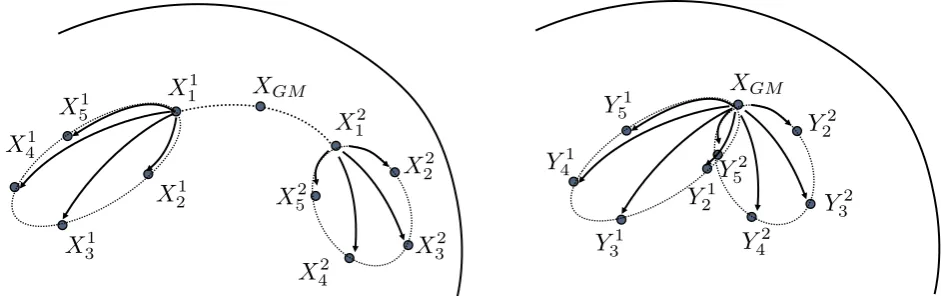
Fig. 1 The Levi Civita parallel transport (left) and a parallel transport that preserves the affine component (right) in the configuration space.
1
X
11X
21X
31X
41X
51X
12X
22X
32X
42X
52Y
12Y
22Y
32Y
42Y
52Y
12Y
22Y
32Y
42Y
52X
GM1
X
11X
21X
31X
41X
51X
12X
22X
32X
42X
52Y
12Y
22Y
32Y
42Y
52Y
12Y
22Y
32Y
42Y
52X
GM1
X
11X
21X
31X
41X
51X
12X
22X
32X
42X
52Y
12Y
22Y
32Y
42Y
52Y
12Y
22Y
32Y
42Y
52X
GM1
X
11X
21X
31X
41X
51X
12X
22X
32X
42X
52Y
12Y
22Y
32Y
42Y
52Y
12Y
22Y
32Y
42Y
52X
GM1
X
11X
21X
31X
41X
51X
12X
22X
32X
42X
52Y
12Y
22Y
32Y
42Y
52Y
12Y
22Y
32Y
42Y
52X
GM1
X
11X
21X
31X
41X
51X
12X
22X
32X
42X
52Y
12Y
22Y
32Y
42Y
52Y
12Y
22Y
32Y
42Y
52X
GM1
X
11X
21X
31X
41X
51X
12X
22X
32X
42X
52Y
12Y
22Y
32Y
42Y
52Y
12Y
22Y
32Y
42Y
52X
GM1
X
11X
21X
31X
41X
51X
12X
22X
32X
42X
52Y
12Y
22Y
32Y
42Y
52Y
12Y
22Y
32Y
42Y
52X
GM1
X
11X
21X
31X
41X
51X
12X
22X
32X
42X
52Y
12Y
22Y
32Y
42Y
52Y
12Y
22Y
32Y
42Y
52X
GM1
X
11X
21X
31X
41X
51X
12X
22X
32X
42X
52Y
12Y
22Y
32Y
42Y
52Y
12Y
22Y
32Y
42Y
52X
GM1
X
11X
21X
31X
41X
51X
12X
22X
32X
42X
52Y
12Y
22Y
32Y
42Y
52Y
12Y
22Y
32Y
42Y
52X
GMWednesday, March 22, 17
1
X
11X
21X
31X
41X
51X
12X
22X
32X
42X
52Y
12Y
22Y
32Y
42Y
52Y
12Y
22Y
32Y
42Y
52X
GM1
X
11X
21X
31X
41X
51X
12X
22X
32X
42X
52Y
12Y
22Y
32Y
42Y
52Y
12Y
22Y
32Y
42Y
52X
GM1
X
11X
21X
31X
41X
51X
12X
22X
32X
42X
52Y
12Y
22Y
32Y
42Y
52Y
12Y
22Y
32Y
42Y
52X
GM1
X
11X
21X
31X
41X
51X
12X
22X
32X
42X
52Y
12Y
22Y
32Y
42Y
52Y
12Y
22Y
32Y
42Y
52X
GM1
X
11X
21X
31X
41X
51X
12X
22X
32X
42X
52Y
12Y
22Y
32Y
42Y
52Y
12Y
22Y
32Y
42Y
52X
GM1
X
11X
21X
31X
41X
51X
12X
22X
32X
42X
52Y
11Y
21Y
31Y
41Y
51Y
12Y
22Y
32Y
42Y
52X
GM1
X
11X
21X
31X
41X
51X
12X
22X
32X
42X
52Y
11Y
21Y
31Y
41Y
51Y
12Y
22Y
32Y
42Y
52X
GM1
X
11X
21X
31X
41X
51X
12X
22X
32X
42X
52Y
11Y
21Y
31Y
41Y
51Y
12Y
22Y
32Y
42Y
52X
GM1
X
11X
21X
31X
41X
51X
12X
22X
32X
42X
52Y
11Y
21Y
31Y
41Y
51Y
12Y
22Y
32Y
42Y
52X
GMWednesday, March 22, 17
Fig. 2 Data Centering via Direct Transport. Left: Before shape data centering; Right: After the shape data centering.
alignment able to generate TPS-horizontal vectors. We name such types of alignment Modified OPA (MOPA). While OPA was based on the minimization of the Eu-clidean size-and-shape distance dS, MOPA is based on the minimization of the TPS pseudo-distance defined as:
dT P S([X]S,[Y]S) = inf Q∈SOm
p
gX((Y Q−X),(Y Q−X)).
In particular the MOPAaligned configurationXˆbis ob-tained by means of an optimal rotation Qˆ minimizing
dT P S.
ˆ
Y =YQˆ
where ˆQ= argmin gX((Y Q−X),(Y Q−X)). Accord-ing to this definition, ˆQ turns out to be the rotational component of the polar decomposition of (A−I), the TPS uniform component of the deformation vectorY−
X. Based on this definition, aligning a shape with an-other means filtering rotations out from the uniform part of the deformation; let us remark that rotations, as defined in a standard Procrustes alignment, are not deformation-based.
After the MOPA, the vector ˆY −X results as a TPS-horizontal vector of the tangent space onX. It is
important to note that MOPA alignment makes sense only between near configurations, when the second can be considered as a small deformation of the first. On the other hand OPA alignment continues to be the main in-strument to superimpose different bodies, characterized by very different shapes.
We now propose a Riemannian Data Centering to analyze sequences of configurations, based on the fol-lowing algorithm (see Fig. 2). Let us considerndifferent sequences (X1j, X2j, X3j, . . .), withj= 1, . . . , n; then:
1. Hierarchical Procrustes Analysis (HPA):
(a) Within each sequence, select a reference config-uration Xj
c, which can be the first one, or the local mean;
(b) Perform a GPA with no scaling among the se-lected referencesXj
c to find theXGM;
(c) Perform n loops of OPA (or MOPA) with no scaling to unit CS, to align all the shapes of a sequence to its proper referenceXj
c. 2. Parallel transport:
(a) Build the TPS-horizontal (or horizontal) vectors
Vij=Xij−Xj
c;
[image:14.595.93.493.80.190.2] [image:14.595.50.521.240.388.2]