A Meta–Analytic Framework for Efficiently Identifying
1Progression Groups in Highway Condition Analysis
2Rawle Prince 1, Matthew Byrne 2, Tony Parry3
3
ABSTRACT
4
The MML2DS (Minimum Message Length Two Dimensional Segmenter) criterion is 5
a powerful technique for road condition data analysis developed at the Nottingham Trans-6
portation Engineering Centre (NTEC), University of Nottingham. The criterion analyses 7
condition data sets by simultaneously identifying optimum trends in condition progression, 8
the position in time and space of maintenance interventions, longitudinal segments within 9
links, and the error likelihood of each measurement. This is done in an unsupervised man-10
ner via classification and regression models based on the Minimum Message Length met-11
ric (MML). Use of MML, however, often requires an exhaustive comparison of all possible 12
models, which naturally raises considerable search–control issues. This is precisely the case 13
with theMML2DSapproach. This paper presents an efficient meta–analytic framework for 14
controlling the generation ofprogression groups, which considerably reduces the search space 15
prior to the application of MML2DS. This is achieved by identifying ‘founder sets’ of lon-16
gitudinal segments, around which families of segments are likely to be formed. An effective 17
subset of these families is then selected, after which the MML2DS criterion is employed 18
as the final arbiter to determine ultimate model configurations and fits. This approach has 19
proved to be very powerful, resulting in significant improvements in efficiency to the effect 20
that accurate results are obtained in a few minutes where it previously took weeks with much 21
1Yotta, Yotta House, 8 Hamilton Terrace, Leamington Spa, CV32 4LY, Warwickshire. Email:
2And/Orr Limited, 14 Clarendon Street, Nottingham, NG1 5HQ, United Kingdom. Email:
3Nottingham Transport Engineering Centre, Faculty of Engineering, University of Nottingham,
smaller data sets. The indications are that this approach can be applied to other techniques 22
besides MML2DS. 23
INTRODUCTION
24
Road agencies collect expansive data sets of pavement condition, forming the backbone 25
of the asset management systems, which are used to identify various performance indicators 26
and maintenance needs. Very often, the data collected is used to fit time series — termed pro-27
gression rates — in order to better understand surface condition indicators, such as pavement 28
roughness and rutting. A road network under study may have many thousands of kilometres 29
of pavement, typically divided into a series of sections: N ={Si|i∈ {1,2, . . . , m}}.Each sec-30
tion S is subsequently subdivided into a series of discrete–length1 chainsS
i ={Ci1, . . . ,Cin}, 31
where Cij denotes chain j of section i, and data for individual chains would be recorded 32
over a number of measurement intervals, usually years. For instance, a typical chain Cj = 33
{x1, . . . , xp} would comprise a series of measurements xj, recorded at various measurement 34
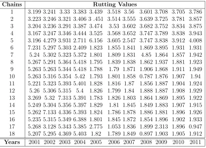
periods, over a number of years. Table. 1 gives an example of simulated rutting data for a 35
1800 meter road segment over an eleven year period. The measurements are often subject 36
to noise or errors which, together with issues of unrecorded maintenance, changes in the 37
measurement devices, as well as possible seasonal variation can combine to make the task of 38
estimating current condition, or identifying true progression rates, very difficult. 39
The MML2DS criterion introduced in (Byrne and Parry 2009) has proved to be very 40
effective in identifying true trends in condition progression, the position in time and space 41
of maintenance interventions, longitudinal segments within links, and the severity of errors 42
among measurements. The key idea was to share data among adjacent chains in a section 43
in order to identify progression groups, GS
i for a section S, formed from chains that can be 44
described by a common progression rate and associated maintenance intervention pattern: 45
S = [
G∈GS i
G, whereG ={C1, . . . ,Ck}. 46
Ultimately, the criterion also identifies how data in individual measurements within a group 47
relate to the group’s progression rate and maintenance intervention pattern, giving valuable 48
information in terms of possible measurement errors and/or seasonal variation. Fig. 1shows 49
a progression group model for the data in Table. 1. 50
Progression group models in (Byrne and Parry 2009) were identified using Minimum Mes-51
sage Length (MML) inference (Wallace 2005). MML is a powerful technique for inductive 52
inference, residing at the intersection of Information Theory and Statistics, which seeks to 53
minimise an objective function that estimates the validity of an inferred model. Since it 54
was first introduced (Wallace and Boulton 1968), MML has been successfully applied to 55
numerous settings, often outperforming rival techniques. These include, selecting the con-56
figuration of Neural Networks (Makalic et al. 2009), classification of proteins in DNA (Zakis 57
et al. 1994), grouping ordered data (Fitzgibbon et al. 2000), inferring decision graphs (Tan 58
and Dowe 2003), classification of spatial data (Wallace 1998), clustering of protein struc-59
tures (Edgoose et al. 1998) and bushfire prediction using decision trees (Dowe and Krusel 60
1993). The issue with MML, however, is that one can only be certain that the optimum 61
model has been identified after the metric has been applied to all other models. This is very 62
much the case with the MML2DS criterion, especially with regard to the identification of 63
progression groups. Considering all possible models is not an issue when dealing with small 64
sections. However, there is an exponential increase in the number of possible progression 65
group models that can be obtained from a given section, and checking all of them quickly 66
becomes problematic as section lengths increase. Moreover, real world pavement networks 67
can have sections with hundreds or thousands of chains and testing all progression group 68
models in such settings is intractable. 69
This paper presents a meta–analytic framework for pre–processing progression group 70
models in order to mitigate search control issues that arose during the application of the 71
MML2DS criterion. Rather than checking all possible progression group models generated 72
to define initial groups around which progression groups are likely to be formed. These initial 74
groups subsequently form the nucleus of larger groups, which are subsequently evaluated by a 75
fitness function derived from the relationship metric. The ‘fittest’ progression group models 76
are retained, and it is these that are ultimately analysed by the MML2DScriterion. More 77
often that not, the set of progression group models retained is not only significantly smaller 78
than the set of possible progression group models obtainable from a given section, but also 79
contains the desired model. Hence, checking this reduced set with theMML2DS criterion 80
generally leads to a result considerably faster that would otherwise be the case. 81
This approach can be thought of as a form of subspace clustering (Vidal 2011), and is 82
comparable to heuristic techniques typically used to deal with combinatorial explosion in 83
this setting (Aggarwal et al. 1999; Kriegel et al. 2005). The speed–ups in the analyses were 84
considerable, especially when it came to large sections, returning results in a few minutes 85
where it previously took weeks, whilst maintaining the required level of accuracy. 86
The paper is organized as follows. The next section provides a detailed presentation of the 87
meta–analytic framework together with algorithms for its implementation. The section that 88
follow discusses results and outputs obtained from experiments, while concluding remarks 89
are in the section thereafter. 90
THE META–ANALYTIC FRAMEWORK
91
Suppose a section with n chains S ={C1, . . . ,Cn}is given, where the aim is to determine 92
the number of progression group models that can be generated forS. The number of chains 93
in a progression group can be set to a minimum k, and letm be the number of progression 94
groups that can be obtained from S. The number of possible progression group models 95
obtainable from S, each with m progression groups, can be given by: 96
Φ(m, n) =
1 if m = 0
n−k
P
Φ(m−1, n−i) otherwise.
Consequently, the number of possible ways of combining at leastmchains is given by Ω(m, n): 98
models(m, n) = n/k
X
m=0
Φ(m, n), (2)
99
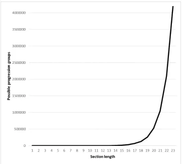
where x/z denotes the integer quotient of x byz. Fig. 2 shows how the number of possible 100
progression group models increases for values of n with k = 1. As can be seen, setting 101
n= 15 yields 16383 possibilities, and increasing n to 21 and 23 yields 1048575 and 4194303 102
possibilities, respectively. This is approximately
O
(1.935)n, so settingn= 60 yields a value 103well over one billion. Generating all of these possibilities on its own can be computationally 104
expensive, and application of the MML2DScriterion to a 5 kilometre section, for instance, 105
using the original approach is clearly not feasible. 106
The Main Idea 107
The technique presented is based on the idea that progression groups are formed around 108
core members, or founder sets, to which other members are subsequently allocated. A 109
relationship metric is employed to discover initial founder sets, which are subsequently re– 110
combined to form a preliminary set of progression group models. Members of this preliminary 111
set are then tested using a sort of fitness function obtained by estimating the strength of 112
the stated relationship among members of a progression group, averaged over all progression 113
groups in a model, and are selected or discarded based on how they compare to previously 114
tested progression group models. It is this reduced set of progression group models, with 115
closely related members, that is submitted to MML2DS criterion for final analysis. The 116
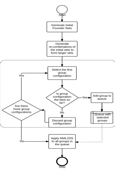
algorithm is shown inFig. 3. 117
As shown in Fig. 3, given a section S the founder sets Sx = {X
1,X2. . .Xn} for S are 118
first calculated, where each Xi = {Ci1, . . . ,Cin} is a close set of chains subject to a stated 119
meta–relationship and tolerance, such that S = [ X ∈Sx
X. Let N ={Si|i ∈ {1,2, . . . , m}} be 120
a network under study. R ∈ C × C →Ris a meta–relationship forN if there is a least upper 121
defined such thatτ denotes the strongest possible relationship under R. A close set subject 123
to a given meta–relationship is subsequently defined as follows. 124
Definition 1 (close set) Let X be a set of chains in a section S and R ∈ C × C → R the 125
meta–relationship on the network containing S. For a given tolerance η, where η < τ, X is 126
a η–close set of chains, subject to R, if ∀x, y ∈ X.R(x, y)∈[η, τ].
127
Since founder sets are intended to initiate progression groups, and not replace them, the 128
relationship metric R should satisfy a necessary condition for the formation of progression 129
groups. For instance, if ∀x ∈ Ci, y ∈ Cj. x =6 y, but Ci and Cj share the same mean and 130
standard deviation, it would be very likely that corr(Ci,Cj) ∈ [η,1], where corr denotes 131
the Pearson correlation coefficient and η some value between 0 and 1 which specifies a 132
high likelihood of closeness relative to the standard deviation — e.g. 0.85 for standard 133
deviation 1.5. Once the founder sets have been identified, a set of progression group models 134
G={GS
x 1 . . .GS
x
n } is then generated fromSx by considering all re–combinations ofSx such 135
that each GSx
i ={Gi1, . . . ,Giq}, and Gik is a union of founder sets. 136
Depending on the definition ofR and the value ofτ, the number of elements inGcan be 137
very large, so relying solely on the generation of founder sets can result in little improvement 138
over employing the MML2DS criterion to all possible progression group models. The next 139
step, therefore, is to build a smaller set of potential progression group models for analysis 140
by the MML2DS criterion in such a way that the cardinality of the reduced set is likely 141
to be considerably less than the number of possible progression group models that can be 142
generated from S. This is achieved by first defining the connectedness of a progression 143
group, which is then averaged over all groups in a progression group model to estimate a 144
‘fitness’ score for the progression group model. 145
nectedness of the chains in G, subject to R, is given by 147
con(G) =
λ if k < 2
k−1
X
i=1
g(G[i],G[i+ 1])
k−1 otherwise
(3) 148
where λ is a default value for groups with less than 2 chains, G[i] is the ith chain in G and 149
g(a, b) = |R(a, b)−τ|, for a 6=b and a adjacent to b. 150
Note that since τ is the upper bound on R it follows that for a given progression group G, 151
the proximity of con(G) to 0 is proportional to the strength of the relationships between 152
adjacent chains in G. Correspondingly, (4) provides a means of quantifying the strength of 153
relationships within a progression group modelGSx
i obtained from a sectionS, based on the 154
connectedness of progression groups within it. 155
conM(GS
x
i ) = m
X
j=1
con(Gij)
m , (4)
156
where m is the cardinality of GSx
i . Consequently, conM can be thought of as a fitness
157
function for progression group models, and is employed so that increasingly ‘fitter’ models 158
will ‘survive’ in order to be examined by the MML2DS criterion. 159
Implementation 160
Although the technique was developed in the context of the MML2DS criterion, it 161
is clearly applicable to settings where other metrics may be employed. It was therefore 162
implemented as a generic, higher–order function which takes the following inputs:2
163
1. a generic list of elements to combine. In the context of theMML2DS criterion, this 164
list is instantiated to a list of arrays denoting a section, where each array represents 165
measurements over a finite number of years for a given chain in the section. 166
2An example implementation in C# is available online (Prince 2015), as well as a demonstration of the
2. a function representing the relationship metric which takes as input a pair of values 167
of the type contained in the input list, and returns a real number.3
168
3. a value for the upper bound (or denoting the strongest relation) of the relationship 169
function. 170
4. a value for the tolerance η used to identify founder sets. 171
5. a specification of the comparison operation to be used when selecting progression 172
group models for final analysis. 173
The function outputs a list containing lists of lists of elements from the input list. For 174
instance, the output in the context of the MML2DS criterion is a list of progression group 175
models, each of which is represented by a list of list of arrays.4 176
Notation The notation used in the algorithms below is as follows. Lists are denoted by 177
square brackets, for example [R] is a list of real numbers and [X] a list of any type X. [] 178
denotes an empty list or sequence, while subscripts are used to refer to elements in a list, 179
for instancexs2 refers to the second element of the listxs. len is a function that returns the
180
length of a list. Given a value x and a listxs, (x::xs) is a list with x added to the front of 181
xs, while (x <>xs) is (x::xs) providing thatx is not already at the front of xs: 182
(x <>xs) =
(x::xs) if xs = []∨xs1 6=x
xs otherwise.
183
For a given listxs and some integer i, xs(≤i) and xs(> i) denote the first ivalues of xs and 184
the remaining values of xs, respectively. Finally, maxLen takes a list of lists as input and 185
returns the length of longest element in the input list. 186
3This is represented as a function delegate in (Prince 2015) while a function pointer can be used in
languages such as C or C++.
4The implementation in (Prince 2015) returns an additional value denoting the number of founder sets
Algorithm 2.1 Algorithm for identifying founder sets. The main function, founders is called with acc = [].
Function: founders(ls,R, τ,ac) if ls = [] then
return acc
else if len(ls) = 1 then als ←(ls1 ::acc)
return als else
efs ←gps(1,ls,ls1,R, τ,[])
m←maxLen(efs) ft ←ls(≤m) bk ←ls(> m) acf ←(ft ::ac)
return founders(bk,R, τ,acf) end if
Function: gps(n,ls, e,R, τ,acc) Require: n≥0∧acc 6= []
if (n >len(ls)−1)then return acc
else
xs ←ls(≤n)
valid ← ∀x∈xs.R(e, x)≤τ
if not valid then return acc else
ys ←(xs ::acc)
return gps(n+ 1,ls, e,R, τ,ys) end if
end if
Identifying founder sets 187
The function to identify founder sets is shown in Algorithm. 2.1. It takes the input 188
list (i.e. the representation of the section S), the relationship metricR, the toleranceτ and 189
a list which serves as an accumulator. An auxiliary function gps is used to identify a block 190
Bi of elements such that ∀x∈Bi.R(a, x)≤τ, wherea is the first element in the list. Each 191
Bi identified is a founder set, and is subsequently removed from the list and added to the 192
accumulator. The function is then applied recursively to the remaining elements of the input 193
list and the accumulated Bis are returned when the input list is empty. 194
Re–combining founder sets 195
The algorithm used to recombine founder sets to form progression group models, shown 196
in Algorithm. 2.2, is based on (2). The main function allGroups implements (2) with 197
k = 1. It re–combines the founder sets by accumulating the group models withigroups that 198
can be formed from a listxs, where i= 1,2, . . . ,len(xs), and where the group models with i
199
elements that can be formed from xs are given by the function ngroups, which implements 200
(1). To form a group model withnelements from a listxs, with each group within the model 201
the first j elements of xs then recursively forms n−1 groups from the remaining ls(> j). 203
The subsidiary groups are then combined with previous ones to form a group model with j
204
groups, and each group model is subsequently added to the accumulator. 205
Algorithm 2.2 Calculating the possible groups from a generic list ls. The main function, allGroups is called withacc = [].
Function: allGroups(xs,acc) Require: xs 6= []
n←len(xs)
for i= 0 to (len(xs)−1) do ys ←ngroups(i,1,xs,[]) for j = 1 tolen(ys)−1 do
acc ←(ysj ::temp) end for
end for return acc
Function: ngroups(n, k,ls,acc) Require: k > 0∧ls 6= []
if n≤0 then
return ([ls] ::acc) else
for i=k to (len(ls)−k) do ft ←ls(≤i), bk ←ls(> i) xs ←ngroups(n−1, k,bk,[]) for j = 1 to len(xs) do
x←xsj, zs ←(ft ::x) if len(zs)≥k then
acc ←(zs ::acc) end if
end for end for return acc end if
Applying the fitness test 206
The list of progression group models returned byAlgorithm. 2.2is then processed using 207
the function mtBy below 208
mtBy(f,ls) =
[] if ls = []
mtByAux(f,xs1,xs(>1),[]) otherwise,
209
where the function mtByAux is given in Algorithm. 2.3. As shown, mtByAux takes a 210
generic list xs, a (fitness) function f to be applied to elements of xs, the first element afrom 211
xs, and an accumulatorzs which serves as the queue inFig. 3. Every subsequent element of 212
ls is compared toa. If an elementy is deemed to be ‘fitter’ than a, it is added to the queue 213
compared to the next element of the list. Comparison in done using the operator compare 215
which specifies the comparison to use when short–listing progression group models to the 216
queue. In accordance with the desired generality of the implementation, given values x and 217
y,compare can be set to either: (i)x < y, (ii)x≤yand (iii)|y−x|< for some∈(0,1). 218
The last option generalises the others in that it allows a group to be added if its fitness score 219
(4) is within a defined proximity of those previously added to the queue.
Algorithm 2.3 Maintaining the ‘fittest’ elements of a list subject to a fitness function f. Function: mtByAux(f, a,xs,zs)
if ls = [] then return zs else
x←xs1, n ←len(xs)
ls ←xs(> n−1)
if compare(f(a), f(x))then
return mtByAux(f, a,ls,(a <>zs)) else
return mtByAux(f, x,ls,(x <>zs)) end if
end if
220
RESULTS AND VISUALISATIONS
221
The framework was evaluated, independently and together with theMML2DScriterion, 222
on simulated data for a number of pavement sections with various lengths, and with prede-223
fined amounts of progression groups and intervention points. Data for each group within a 224
section was randomly sampled from a normal distribution with a unique mean and standard 225
deviation, relative to the other groups within that group. 226
In order to test the framework’s ability to reduce the number of generated progression 227
group models, it was applied to a number of sections without any subsequent analysis. The 228
data in Table. 1was one of these sections. There are two predefined progression groups in 229
this section giving rise to the following progression group model{{C1, . . . ,C5},{C6, . . . ,C18}}
230
as shown in Fig. 1. Applying Algorithm. 2.2 to this section returns 131071 possible 231
settingη = 0.75,τ = 1 and the comparisoncompare such thatcompare(a, b) = |a−b|<0.03, 233
the meta–analytic framework reduces this to 12 possibilities, amongst whichis the expected 234
progression group model.5
235
For all of the sections evaluated, applying the MML2DS criterion to all possible pro-236
gression groups models would have taken days to complete,6 in addition to possible space
237
complexity issues due to the generation of progression group models for long sections. It was, 238
therefore, not feasible to compare the time it took the implementation of theMML2DS cri-239
terion combined with the meta–analytic framework to one without the meta–analytic frame-240
work. Instead, we investigated the trade off between accuracy and efficiency provided by 241
the meta–analytic framework, and so examined the number of founder sets identified, the 242
number of progression groups discovered, and the time it took to complete the analysis. In 243
this way, the aim was to determine if the chosen relationship, the number of founder sets 244
obtained and the subsequent reduction in the time it took to complete the analysis, had 245
any significant impact on the accuracy of the analysis. Results obtained using the Pearson 246
correlation coefficient corr as the relationship R are shown in Table. 2. 247
As these results show, we were able to discover the expected number of progression groups 248
on every occasion, even when the section lengths were very large. These results compare 249
with what was obtained with the original implementation of theMML2DScriterion (Byrne 250
and Parry 2009), but, in this case, results were obtained in less than fifteen minutes, even 251
with the longest sections, where it took upwards of five days for sections with less than 252
60 chains in (Byrne and Parry 2009). While part of this increase in performance can be 253
attributed to our use of parallel programming techniques to exploit multi–core architectures 254
during interactions of piecewise and mixture models, the identification of founders sets, and 255
the subsequent selection of progression groups based on connectedness, considerably reduced 256
the number of cases to be checked by the MML2DS criterion, and was clearly the main 257
5Note, this example is implemented in (Prince 2015).
6The tests were done on a 64 bit Windows 7 machine with 8GB RAM and an Intel Core i7–4800, 2.7GHz
reason for the performance improvements. 258
This also shows that the meta–analytic framework does provide an effective technique for 259
balancing the trade–off between efficiency and accuracy during the application of MML anal-260
ysis. Moreover, not only can the meta–relationship function be adapted to different settings, 261
but the parameters, for controlling the relationship’s strength a well as the search space, 262
can also be tailored to performance requirements on different systems, or to different do-263
mains. This approach clearly goes a long way in addressing complexity issues related to the 264
MML2DS criterion, since, as can be seen from Table. 2, the time taken for results to be 265
obtained depends on meta–relationships within the data set — indicated by the number of 266
founder sets discovered — and not necessarily the size of the data set. 267
A major limitation of this approach, however, is that it might not always be straightfor-268
ward to identify a suitable meta–relationship. Our use of the Pearson correlation coefficient 269
was justified since data in each of the predefined progression groups was sampled from the 270
same normal distribution. In other domains, one would expect that a fair amount of domain 271
knowledge and/or experimentation would be required before a suitable meta–relationship 272
can be identified. 273
Visualisations 274
The primary purpose of the meta–analytic framework was to control the generation of 275
progression groups prior to MML2DSanalysis, so outputs obtained from the final system, 276
which employed the MML2DS criterion, corresponded to those obtained in the original 277
application of the MML2DS criterion (Byrne and Parry 2009). As mentioned earlier, the 278
aim of the MML2DS criterion was to identify the progression rates of the condition data. 279
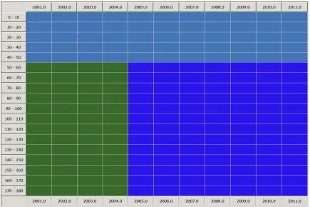
Example results are presented as shown inFig. 5 andFig. 4. The position of maintenance 280
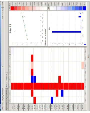
interventions and progression groups are shown in coloured blocks in Fig. 5, whereby each 281
block is a group of adjacent intervals which share a common progression rate. Progression 282
rates for selected intervals and measurement errors (i.e. outliers) are shown at the right, with 283
to the progression trend above it. For example, section 230 – 240 has a clear maintenance 285
intervention occurring between years 2004 and 2005. 286
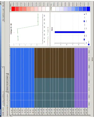
Fig. 4 uses a colour coding to highlight where and when errors in the condition data 287
appear to exist. A deeper shade of red or blue indicate a higher likelihood of erroneous data, 288
where red indicates those above the trend and blue those below the trend. For instance, 289
there is a clear disparity in the measurements data recorded chain 10 – 20 in 2001 and since 290
this is inconsistent with measurements taken in the proceeding and following years, it is 291
highlighted as an error and not caused by a maintenance intervention. This disparity may 292
have been caused, for instance, by a poorly calibrated device which overestimated condition 293
levels along the whole section that year. Fig. 5 also displays the position of measurement 294
errors relative to the progression trend, which is displayed in a similar way to Fig. 4. 295
CONCLUSION
296
This paper presented a meta–analytic framework for pre–processing group permutations 297
generated during the application of theMML2DScriterion. While theMML2DScriterion 298
provides a novel solution to the problem of identifying progression rates, the required sharing 299
of data over adjacent chains raised considerable search control issues, which potentially 300
limited its applicability to real–world settings. 301
By applying a relationship that satisfies a necessary condition for the formation of pro-302
gression groups, and estimating the relative connectedness of progression groups based on 303
this relationship, the proposed meta–analytic framework provides a robust method of re-304
ducing the number of progression group models submitted to the MML2DS criterion for 305
analysis. Empirical test have shown that, depending on the relationship selected and the 306
choice of associated parameters, the set of progression group models retained usually con-307
tain the desired solution. The meta–analytic framework, therefore, provides an efficient and 308
effective approach to managing the trade off between efficiency and accuracy required for 309
applications of theMML2DScriterion, andMMLin general, to real–world settings. There 310
application of different techniques, for example fuzzy logic. Moreover, the framework was 312
implemented as a generic function and can be utilised in different settings, and with vari-313
ous relationship functions. However, some understanding of the data set and the problem 314
domain would be required to make effective use of this approach. 315
The framework also illustrates how novel search control techniques and quality data 316
mining algorithms can be combined to extract information from noisy data sets without any 317
significant loss in accuracy. While the progression rates were the ultimate answer sought 318
by the MML2DScriterion, the progression groups obtained can provide useful information 319
about past maintenance interventions. This would certainly be desirable in situations where 320
maintenance records are not up–to–date, and knowledge of past maintenance can be used 321
to derive strategies for the future. The next step is to apply this combined technique to 322
real–world data, and we are in the process of doing so at present. 323
ACKNOWLEDGEMENT
324
This work was completed when the first and second authors were a research assistant 325
and fellow, respectively, in the Nottingham Transport Engineering Centre, Faculty of En-326
gineering, University of Nottingham. The research was supported by the EPSRC grant 327
APPENDIX I. REFERENCES
329
Aggarwal, C., Wolf, J., Yu, P., Procopiuc, C., and Park, J. S. (1999). “Fast algorithms for 330
projected clustering.” Proceedings of the 1999 ACM SIGMOD International Conference 331
on Management of Data, New York, NY, USA, ACM, 61–72. 332
Byrne, M. and Parry, T. (2009). “Network level pavement condition preparation using Mini-333
mum Message Length.”Twelfth International Conference on Structural and Environmental 334
Engineering Computing. 335
Dowe, D. L. and Krusel, N. (1993). “A decision tree model of bushfire activity.”Proceedings of 336
the 6th Australian Joint Conference on Artificial Intelligence, World Scientific , Singapore. 337
Edgoose, T., Allison, L., and Dowe, D. L. (1998). “An MML classification of protein structure 338
that knows about angles and sequence.” Proceedings of the PACIFIC SYMPOSIUM ON 339
BIOCOMPUTING, World Scientific , Singapore. 340
Fitzgibbon, L. J., Allison, L., and Dowe, D. L. (2000). “Minimum Message Length grouping 341
of ordered data.”Algorithmic Learning Theory, H. Arimura, S. Jain, and A. Sharma, eds., 342
Vol. 1968 of Lecture Notes in Computer Science, Springer Berlin Heidelberg, 56–70. 343
Kriegel, H., Kr¨oger, P., Renz, M., and Wurst, S. (2005). “A generic framework for efficient 344
subspace clustering of high–dimensional data.”Proceedings of the Fifth IEEE International 345
Conference on Data Mining, IEEE Computer Society, 250–257. 346
Makalic, E., Allison, L., and Dowe, D. L. (2009). “MML inference of single–layer neural 347
networks.”Proceedings of the IASTED International Conference on Artificial Intelligence 348
and Applications, 08 September 2003 to 10 September 2003. 349
Prince, R. (2015). “C# implementation on the Meta–Analytic Framework.https://github.
350
com/rawlep/MetaAnalyticFramework/tree/ASCE.
351
Tan, P. and Dowe, D. L. (2003). “MML inference of decision graphs with multi–way joins 352
and dynamic attributes.” AI 2003: Advances in Artificial Intelligence, T. Gedeon and L. 353
Fung, eds., Vol. 2903 of Lecture Notes in Computer Science, Springer Berlin Heidelberg, 354
Vidal, R. (2011). “Subspace clustering.” Signal Processing Magazine, 28(2). 356
Wallace, C. S. (1998). “Intrinsic classification of spatially correlated data.” The Computer 357
Journal, 41(8), 602–611. 358
Wallace, C. S. (2005). Statistical and Inductive Inference by Minimum Message Length. 359
Springer-Verlag (Information Science and Statistics). 360
Wallace, C. S. and Boulton, D. M. (1968). “An Information Measure for Classification.”The 361
Computer Journal, 11(2), 185–194. 362
Zakis, J., Cosic, I., and Dowe, D. (1994). “Classification of protein spectra derived for the 363
Resonant Resonant Recognition model using the Minimum Message Length principle.” 364
List of Tables
366
1 Rutting values(mm) for a 1.8 kilometre section over eleven years. . . 19 367
2 Performance of the meta–analytic technique on a selection of simulated sec-368
tions of various lengths with predefined progression groups (PGs), showing 369
the number of founder sets (F Sets) found withR as the Pearson correlation 370
coefficient, the number of progression groups discovered, and the time taken 371
Chains Rutting Values
[image:19.612.100.516.70.368.2]1 3.199 3.241 3.33 3.383 3.439 3.518 3.56 3.601 3.708 3.705 3.786 2 3.223 3.246 3.321 3.406 3 .451 3.514 3.555 3.639 3.725 3.781 3.857 3 3.204 3.236 3.291 3.387 3.474 3.53 3.602 3.682 3.752 3.834 3.875 4 3.167 3.247 3.346 3.444 3.525 3.568 3.652 3.747 3.789 3.838 3.943 5 3.196 4.279 3.931 2.711 6.156 3.605 2.547 3.747 3.838 3.912 4.008 6 7.231 5.297 5.303 2.409 1.823 1.855 1.841 1.869 3.895 1.931 1.931 7 5.24 5.302 5.323 5.372 1.801 1.809 1.831 4.85 1.864 1.857 1.942 8 5.267 5.291 5.364 5.418 1.795 1.839 1.838 1.862 1.937 1.881 1.923 9 5.263 5.263 5.344 5.418 1.788 1.79 1.871 1.906 1.868 1.911 1.949 10 5.263 5.316 5.354 5.42 1.793 1.801 1.858 0.787 1.876 1.907 1.94 11 5.221 5.323 5.393 5.401 1.828 1.816 1.87 1.856 1.887 1.904 1.924 12 5.26 5.306 5.315 5.4 1.826 1.799 1.84 1.888 1.887 1.908 1.929 13 3.269 5.32 7.313 5.391 1.783 1.826 1.803 1.864 1.869 1.895 1.922 14 5.249 5.304 5.356 5.397 1.829 1.81 1.845 1.849 1.883 1.907 1.915 15 5.262 7.133 4.336 5.393 1.824 1.786 1.878 1.886 1.881 1.896 1.926 16 5.235 5.315 5.349 6.388 1.801 1.845 1.872 1.854 1.896 1.902 1.933 17 5.268 3.128 5.343 5.385 2.775 1.053 1.836 1.899 2.313 1.896 0.947 18 5.207 5.295 4.369 5.403 1.82 1.789 1.849 0.897 1.903 1.905 1.912 Years 2001 2002 2003 2004 2005 2006 2007 2008 2009 2010 2011
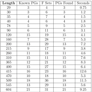
Length Known PGs F Sets PGs Found Seconds
29 3 4 3 0.75
30 3 6 3 1.2
35 4 7 4 1.5
40 4 6 4 1.8
78 5 9 5 2.5
90 6 11 6 3.1
120 15 19 15 4.1
160 7 28 7 5.3
200 13 29 13 7.2
215 9 17 9 3.8
260 11 18 11 4.6
310 15 11 15 7.6
365 12 21 12 8.3
400 15 27 15 6.4
415 16 23 16 12.6
470 10 18 10 5.3
509 18 36 18 11.5
545 13 29 13 5.6
[image:20.612.158.455.69.369.2]604 21 31 21 9.25
List of Figures
373
1 Progression groups for the example section in Table. 1. There are two pro-374
gression groups: (i) from 0 t0 50 meters and (ii) from 50 to 180. The position 375
of maintenance interventions and progression groups are shown in coloured 376
blocks at the left, whereby each block is a group of adjacent 10 meter chains 377
that share the same progression rate. . . 22 378
2 Increase in the number of possible progression group models in relation to 379
section lengths. Section lengths are on the horizontal axis while the number 380
of progression group models that can be generated are on the vertical axis. . 23 381
3 Flowchart depicting the meta–analytic procedure applied to a section. . . 24 382
4 Progression rate and error. . . 25 383
5 Progression groups identified on a section with the fitted progression rates 384
and maintenance intervention patterns. There are three progression groups: 385
(i) from 0 t0 90 meters, (ii) from 90 to 240 meters, and (iii) from 240 to 290. 386
The position of maintenance interventions and progression groups are shown 387
in coloured blocks at the left, whereby each block is a group of adjacent 10 388
meter chains which share the same progression rate. Chain 230−240 has 389
been selected, showing a clear maintenance intervention occurring between 390
years 2004 and 2005 and this intervention pattern exists across all chains 391
FIG. 5. Progression groups identified on a section with the fitted progression rates and maintenance intervention patterns. There are three progression groups: (i) from