Collisionless distribution function for the relativistic force free Harris sheet

Collisionless distribution function for the relativistic force-free Harris sheet

C. R. Stark1,a) _{and T. Neukirch}1,b)

School of Mathematics and Statistics, University of St Andrews, St Andrews, KY16 9JT, United Kingdom

(Dated: 10 November 2011)

A self-consistent collisionless distribution function for the relativistic analogue of the force-free Harris sheet is presented. This distribution function is the relativistic gen-eralization of the distribution function for the non-relativistic collisionless force-free Harris sheet recently found by Harrison and Neukirch [Phys. Rev. Lett. 102, 135003 (2009)] as it has the same dependence on the particle energy and canonical momenta. We present a detailed calculation which shows that the proposed distribution function generates the required current density profile (and thus magnetic field profile) in a frame of reference in which the electric potential vanishes identically. The connection between the parameters of the distribution function and the macroscopic parameters such as the current sheet thickness is discussed.

PACS numbers: 52.20.-j, 52.25.Xz, 52.55.-s, 52.65.Ff Keywords: Suggested keywords

I. INTRODUCTION

Force-free plasma equilibria, i.e. plasma equilibria for which the current density is aligned with the magnetic field lines, are of great importance in both astrophysical and laboratory plasmas, in particular for modelling low-β systems. Within the framework of magnetohy-drodynamics (MHD) a large number of analytical force-free equilibria are known.1–3

For collisionless plasmas, with equilibria being solutions of the time-independent Vlasov-Maxwell (VM) equations, the situation is completely different. So far only a small number of one-dimensional (1D) collisionless force-free plasma equilibria is known, of which most belong to the class of linear force-free fields4–8_{. So far, analytical self-consistent distribution} functions have been found only for one example of non-linear force-free fields, the force-free Harris sheet9–12_{. Finding self-consistent force-free collisionless equilibria is difficult, because} one is dealing with an inverse problem, i.e. find a solution of the Vlasov equation for a given magnetic field and electric current system (for a discussion of the problem see Ref. 10).

The equilibria mentioned in the previous paragraph have all been found for the non-relativistic regime. It is the aim of this paper to investigate whether it is possible to generalize the distribution function found for the force-free Harris sheet into the relativistic regime. We define the relativistic force-free condition as JµFµν = 0, where Jµ is the four-current density and Fµν the electromagnetic four-tensor. If a frame of reference exists in which the electric field vanishes the relativistic force-free condition is identical with the non-relativistic force-free condition J×B =0 in this frame of reference.

Collisionless equilibria of the type we are trying to calculate in this paper could be of importance for investigations of physical processes like instabilities or magnetic reconnection in relativistic plasmas (see e.g. Refs 13–21). In order to find the relativistic generalization of the collisionless distribution function for the force-free Harris sheet, we shall use the relativistic version22–24 of the distribution function of the normal Harris sheet25 as a guide, together with the non-relativistic distribution function for the force-free Harris sheet.9,11

II. THE NON-RELATIVISTIC FORCE-FREE HARRIS SHEET

In a 1D VM equilibria with translational symmetry, it is assumed that all plasma variables depend only on one spatial coordinate, here taken to bez and that the magnetic flux density has componentsBx and By. The magnetic flux density components can be written in terms of the vector potential A= (Ax, Ay, Az) where,

Bx =− dAy

dz , (1)

By = dAx

dz , (2)

and the electric field is the gradient of the electric potentialϕ, E=−∇ϕ=−dϕ

dzˆz. (3)

These relations automatically satisfy Faraday’s law ∇ × E = 0 and Gauss’ law for the magnetic flux density ∇ ·B = 0. Due to the symmetries of the system (time and spatial independence of xandy) the three obvious constants of motion for each particle species are the Hamiltonian or particle energy for each species s,

Hs = 1 2ms(v

2 x+v

2 y +v

2

z) +qsϕ, (4)

and the canonical momentum in the x and y directions respectfully,

pxs=msvx+qsAx, (5)

pys=msvy+qsAy, (6)

where ms and qs are the mass and charge of each species. Here, we consider a plasma composed of two species of equal and opposite charge but of differing mass, that is, elec-trons and protons. All positive functions fs satisfying the appropriate conditions for the existence of the velocity moments and depending only on the constants of motion, fs = fs(Hs, pxs, pys) solve the steady-state Vlasov equation. For a quasi-neutral plasma in force balance, Amp`ere’s law can be written as

d2Ax

dz2 =−µ0

∂Pzz ∂Ax

, (7)

d2Ay

dz2 =−µ0

∂Pzz ∂Ay

where Pzz(Ax, Ay) is the zz-component of the plasma pressure tensor, Pzz =

∑

s ∫ _∞

−∞

msv2zfsd3v. (9)

The magnetic flux density components of the force-free Harris sheet are given by

Bx =B0tanh (z/λ), (10)

By =

B0

cosh (z/λ). (11)

The x−component of the magnetic flux density has the same spatial structure as the Harris sheet, but whereas the Harris sheet is kept in force balance by pressure gradients, the force-free Harris sheet maintains force balance via a magnetic shear y−component.

Assuming that the pressure takes the form Pzz(Ax, Ay) = P1(Ax) + P2(Ay), equa-tions (7) and (8) combined with the force-free condition (B2

x +By2 = const.) gives the condition for force balance:

( dAx

dz )2

+ 2µ0P1(Ax) = 2µ0P01, (12) (

dAy dz

)2

+ 2µ0P2(Ay) = 2µ0P02, (13) whereP01 and P02 are constants. Solving these equations forP1(Ax) andP2(Ay) the plasma pressure for the force-free Harris sheet is

Pzz = B₀2

2µ0 [

1 2cos

( 2Ax B0λ

) + exp

( 2Ay B0λ

)]

+P03, (14)

whereP03 is a constant. Since the pressure is the sum of two independent functions that are a function of Ax and Ay respectively, the distribution function is assumed to be of the form fs= exp (−βsHs)[g1s(pxs) +g2s(pys)], (15) where the reciprocal thermal energy of species s is βs = (kBTs)−1. Applying Channell’s fourier transform method5_{, echoed in Harrison and Neukirch}9_{, the plasma pressure integral} can be solved for the distribution functionfs. Therefore, a collisionless distribution function for the force-free Harris sheet is

fs = n0,s v3

th,s

exp (−βsHs)[ascos (βsuxspxs)

III. RELATIVISTIC FORCE-FREE HARRIS SHEET

If the thermal energy of the plasma, kBT, approaches or exceeds the rest energy, mc2, a non-relativistic treatment is no longer sufficient to describe the system. In a relativistic framework, Pν _{are the components of the canonical momentum four-vector P = p+q}

sA,

where: p=mw= (E/c, p1_{, p}2_{, p}3_{) is the four-momentum; w= (w}0_{, w}1_{, w}2_{, w}3_{) is the} four-velocity; andA= (ϕ/c, A1, A2, A3) is the four-potential. The Hamiltonian or particle energy for each species s, Hs corresponds to the speed of light times the zeroth component of the canonical momentum four-vector P0_c=E+q

sϕ. The subsequent canonical components are now functions of the four-velocity,Pi =mswi+qsAi. A relativistic analogue of the force-free Harris sheet distribution function can be written as

fs =fs0exp (−βsP0c)[ascos (βsuxsP1)

+ exp (βsuysP2) +bs], (17)

wherefs0 =n0smsβs/(4πc) andn0sis the mean particle density. Details of the normalisation calculation are given in appendix A. Using the relation cosx = 1₂(eix+e−ix) we can recast the distribution function as

fs=f1s(w0, w2) +f2s(w0, w1) +f3s(w0, w1) +f4s(w0) =fs0[c1sexp (−cβsms(w0 −uysw2/c))

+c2sexp (−cβsms(w0+iuxsw1/c)) +c3sexp (−cβsms(w0−iuxsw1/c))

+c4sexp (−cβsmsw0)], (18)

where

c1s = exp (−βsqs(ϕ−uysA2)), (19) c2s =

as

2 exp (−βsqs(ϕ+iuxsA

1_{)), (20)}

c3s = as

2 exp (−βsqs(ϕ−iuxsA

1_{)), (21)}

c4s =bsexp (−βsqsϕ). (22)

(Tαβ₎

plasma+ (Tαβ)em, incorporating contributions to the energy and momentum from the kinetic and electromagnetic behaviour of the plasma. In this context, a relativistic force-free system corresponds to Tαβ

,β =−JβFαβ = 0, where Fαβ are the components of the Faraday tensor and J = (cρ, J1, J2, J3) is the four-current. In a frame where ϕ = 0, B = (B1, B2,0) andJ= (cρ, J1_{, J}2_{,0), the only non-zero component of the Lorentz force isJ}

1B2−J2B1 = 0. Neglecting viscosity and heat conduction the 33-component of (Tαβ₎

plasma, which we will refer to as the plasma pressure P, is given by

P =c∑ s

ms ∫

d4w (w3)2fs(w)δ(wνwν −c2) (23) =c∑

s

(P1s+P2s+P3s+P4s). (24)

Note that (Tαβ₎

plasma = pαNβ, where N = nu is the number flux four-vector and n is the number density. To solve the first pressure integral P1s we will perform a coordinate transformation defined by the transformation matrix

[Λβ_α¯] =       

γ1s 0 −uysγ1s/c 0

0 1 0 0

−uysγ1s/c 0 γ1s 0

0 0 0 1

       , (25)

where γ1s = (1 −u2ys/c2)−1/2, w ¯

β _{= Λ}β¯

αwα and wα = Λα_β¯w ¯

β _{such that Λ}β¯

αΛα_β¯ = 1. Note that this coordinate transformation, and following transformations, are used as a means to evaluate the integral and do not physically correspond to a Lorentz boost. The Jacobian of the system is simply J = 1 therefore, dwβ¯_=dwα _{and f}

1s(w0, w2) = f1s(w ¯

0_{). Making the} change of variables yields

P1s =ms ∫

d4w¯ (w¯3)2f1s(w ¯ 0_)δ(w

νwν −c2), (26)

which can be written as

P1s =ms ∫

d3w¯ (w ¯ 3₎2

w¯0 f1s(w ¯ 0

), (27)

where

f1s=fs0c1sexp (−cβsmsw ¯ 0_/γ

1s). (28)

A convenient way of expressing w¯0 can be obtained using the inner product of the four-velocity with itself, w·w = gµνwνwµ which gives w

¯

here is defined as gµν =diag(+1,−1,−1,−1). The integral can now be easily evaluated by changing to spherical coordinates, making use of the J¨uttner transformation (w/c = sinhx) and using the known integral26

∫ _∞

0

sinh2νx exp (−βcoshx)dx

= √1

π (

2

β )ν

Γ(ν+1₂)Kν(β), (29) where K is the modified Bessel Function of the second kind. Therefore

P1s =

k1sn0s βsc

exp (−βsqs(ϕ−uysA2)), (30) wherek1s=γ12sK2(Λ1s) and Λis =msc2βs/γis. SimilarlyP2s and P3s can be evaluated using the following coordinate transformation

[∆β_α¯] =       

γ2s ±iuxsγ2s/c 0 0 ±iuxsγ2s/c γ2s 0 0

0 0 1 0

0 0 0 1

       , (31)

where γ2s = (1 +u2xs/c2)−1/2, w ¯

β _{= ∆}β¯

αwα and wα = ∆α_β¯w ¯

β _{such that ∆}β¯

α∆α_β¯ = 1. The Jacobian is again J = 1, with f2s(w0, w1) =f2s(w

¯

0_{) and f}

3s(w0, w1) = f3s(w ¯

0_{). This yields}

P2s =

k2sn0s 2βsc

exp (−βsqs(ϕ+iuxsA1)), (32) P3s =

k2sn0s 2βsc

exp (−βsqs(ϕ−iuxsA1)), (33) wherek2s =asγ22sK2(Λ2s). The final pressure integralP4scan be trivially evaluated, without any need for a coordinate transformation, using Eq. (29) yielding

P4s=

k3sn0s βsc

exp (−βsqsϕ), (34)

where k3s =bsK2(Λ3s) and Λ3s =msc2βs. The total plasma pressure is then

P =∑

s

n0sk1s βs

exp (−βsqsϕ)[exp (βsqsuysA2)

+ (k2s/k1s) cos (βsqsuxsA1) +k3s/k1s]. (35) The charge density ρ is given by (see Eq.(B5)),

ρ=−∂P

∂ϕ = ∑

s

where,

Ns(A1, A2) = n0sk1s[exp (βsqsuysA2) +(k2s/k1s) cos (βsqsuxsA1)

+k3s/k1s]. (37)

A charge neutral plasma requires that ρ= 0, hence

ϕ = 1

e(βi+βe) ln

( Ni Ne

)

. (38)

The condition of vanishing electric field is satisfied by Ne =Ni, which is true if

βiuyi=−βeuye, (39)

βi|uxi|=βe|uxe|, (40)

n0ik1i =n0ek1e =n0, (41)

k2i/k1i =k2e/k1e=a, (42)

k3i/k1i =k3e/k1e=b. (43)

As a result the plasma pressure is given by

P = (βi+βe)

βiβe

n0[exp (−βeeuyeA2)

+acos (βeeuxeA1) +b]. (44) The x−and y− components of the current density are calculated using Eqs. (B6) and (B7) (see Appendix B)

J1 = ∂P

∂A1 =−

(βi+βe) βi

n0aeuxesin (βeeuxeA1), (45) J2 = ∂P

∂A2 =−

(βi+βe) βi

n0euyeexp (−βeeuyeA2). (46) The corresponding, self-consistent vector potential can be obtained via Amp`ere’s Law,

d2A1

dz2 =−µ0J 1

, (47)

d2A2

dz2 =−µ0J 2

. (48)

The resulting vector potential components can be written as,

A1 =α1arctan (exp (z/λ1)), (49)

and the magnetic flux density components are

B1 =−(2α2/λ2) tanh (z/λ2), (51)

B2 = α1/(2λ1) cosh (z/λ1)

, (52)

where

α1 = 4/(βeeuxe), (53)

α2 = 1/(βeeuye), (54)

λ1 = (

βi

βe(βi+βe)aµ0n0e2u2xe )1/2

, (55)

λ2 = (

2βi

βe(βi+βe)µ0n0e2u2ye )1/2

. (56)

For a force-free system we require J1B2 −J2B1 = 0. This condition is satisfied provided 4α2 =±α1 (α =|α1|) and λ1 =λ2 =λ which implies uxe =−uye and a = 1/2. Therefore, the relativistic force-free Harris sheet is

B1 =B0tanh (z/λ), (57)

B2 = B0

cosh (z/λ), (58)

whereB0 =α/(2λ). The relationship between the microscopic and macroscopic parameters of the equilibria can be deduced by comparing Eq. (14) to Eq. (44). This yields

B2 0 2µ0

=n0

(βi+βe) βeβi

, (59)

a= 1

2, (60)

P03=n0

(βi+βe) βeβi

b, (61)

2

|B0|λ =eβe|uxe|=eβi|uxi|, (62)

2

B0λ

=−eβeuye=eβiuyi, (63)

where we have assumed that λ is positive and B0 can be negative. Following Neukirch et al.11 _{the connection with the original Harris sheet can be made using Eq. (59) and Eq. (63)} to obtain an expression for λ,

λ= (

2(βe+βi) µ0e2βeβin0(uyi−uye)2

)1/2

Therefore, the relativistic free Harris sheet is equivalent to the non-relativistic force-free Harris sheet9–12 _{(and consistent with the relativistic Harris sheet}22_{) where we can now} formally access the relativistic regime, msc2βs≪1.

When msc2βs ≫ 1 the relativistic solution reduces to its non-relativistic counterpart where,

n0 =n0sγ12sK2(Λ1s)≈α1exp (

msβsu2ys 2

)

, (65)

a= asγ 2

2sK2(Λ2s) γ2

1sK2(Λ1s) ≈α2exp

(

−msβs 2 (u

2

xs+u2ys) )

, (66)

b= bsK2(Λ3s)

γ2

1sK2(Λ1s)

≈α3exp (

−msβsu2ys 2

)

, (67)

and

α1 =n0s(1 +u2ys/c2)(1 +u2ys/(4c2)) ×

( π

2msβsc2 )1/2

exp(−msβsc2 )

, (68)

α2 =as

(1−u2 xs/c2) (1 +u2

ys/c2)

(1−u2

xs/(4c2)) (1 +u2

ys/(4c2))

, (69)

α3 =bs

(1−u2

ys/(4c2)) (1 +u2

ys/c2)

. (70)

This is consistent with Neukirch et al.11_{. In the ultra-relativistic regime m}

sc2βs≪1 and n0 ≈

2n0s (msc2βs)2

(1−u2_ys/c2)−2, (71)

a≈as (

1−u2 ys/c2 1 +u2

xs/c2 )2

= 1

2, (72)

b ≈bs(1−u2ys/c

2₎2_{. (73)}

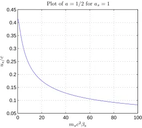
The general solution is constrained by the condition

a= asγ 2

2sK2(Λ2s) γ2

1sK2(Λ1s) = 1

2, (74)

0 20 40 60 80 100 0.05

0.1 0.15 0.2 0.25 0.3 0.35 0.4 0.45

msc2βs us

/

c

Plot of_a= 1_/2 for_as= 1

FIG. 1. Plot of us against msc2βs foras= 1, exhibiting the relationship a= 1/2 that constrains

the relativistic force-free Harris sheet.

IV. SUMMARY AND CONCLUSIONS

Recently the first nonlinear force-free, non-relativistic VM equilibrium for the force-free Harris sheet was reported by Harrison and Neukirch9_{. If the thermal energy of the plasma} approaches or exceeds its rest energy, a non-relativistic treatment is no longer sufficient and a relativistic analogue must be sought. This paper has presented a collisionless distribution function for the relativistic force-free Harris sheet. Mirroring the non-relativistic solution9–11, where the properties of the pressure tensor were exploited, the energy-momentum tensor

Tαβ _{was wielded in an equivalent role}27_{, allowing the calculation of the equilibrium. In our} calculation, we restrict ourselves to a frame where the electric potential vanishes (ϕ = 0), B = (B1_{, B}2_{,0), andJ = (cρ, J}1_{, J}2_{,0), where the only non-zero component of the Lorentz} force is J1B2−J2B1 = 0. The condition of vanishing electric field is true only in one frame of reference; in a moving frame ϕ is non-zero. The resulting relativistic force-free Harris sheet is identical to its non-relativistic counterpart but now the relativistic regime where

msc2βs≪1, can be formally accessed.

Suzuki explored possible equilibria by describing the deviation of the distribution function from a Maxwell-J¨uttner distribution using orthogonal polynomial series28_{. Using this novel} method a new, two dimensional equilibrium was reported. Kocharovsky and co-workers use the method of invariants of particle motion to find exact solutions of the VM system for arbitrary particle energy distributions29–31_{. There technique allows for the description of} multicomponent plasmas, that may be relativistic or not, for a general magnetic geometry29_.

Relativistic equilibria have also been studied extensively within the context of plasma pinches and electron beams used in fusion and laboratory plasmas35–42_{. In these} inves-tigations an electron beam, described by a prescribed distribution function, is embedded in a background plasma permeated by a background magnetic field. The resulting elec-tromagnetic fields are self-consistently calculated yielding stable Vlasov equilibria. A va-riety of tailored seed distribution functions have been investigated such as monoenergetic distributions35,36_{; warm beams (i.e. a drifting Maxwellian)}37,38_{; and helical (force-free) beams} (i.e. a combination of axial and azimuthal configurations)38–42_.

The work presented here lays the critical bedrock for further investigations of plasma phe-nomena such as waves, instabilities and magnetic reconnection. In particular the distribution function reported here can be used as the initial conditions for numerical investigations of magnetic reconnection in relativistic, collisionless plasmas.

ACKNOWLEDGMENTS

Appendix A: Normalisation Constant, fs0

Consider the distribution function,

fs=f1s(w0, w2) +f2s(w0, w1) +f3s(w0, w1) +f4s(w0) =fs0[c1sexp (−cβsms(w0 −uysw2/c))

+c2sexp (−cβsms(w0+iuxsw1/c)) +c3sexp (−cβsms(w0−iuxsw1/c))

+c4sexp (−cβsmsw0)], (A1)

where

c1s = exp (−βsqs(ϕ−uysA2)), (A2) c2s =

as

2 exp (−βsqs(ϕ+iuxsA

1_{)), (A3)}

c3s = as

2 exp (−βsqs(ϕ−iuxsA 1

)), (A4)

c4s =bsexp (−βsqsϕ). (A5)

The four-current density Jµ_{= (cρ, J}1_{, J}2_{, J}3_{) is defined as}

Jµ=c∑ s

qs ∫

d4w wµfs δ(wνwν−c2). (A6)

To evaluate the normalisation constant fs0, we make use of the zeroth component of the four-current (the charge density ρ=∑_sqsns) to calculate the charge number density,

n0sn˜ = ∫

d4w w0fs δ(wνwν −c2) (A7) =n1s+n2s+n3s+n4s, (A8) where n0s is the mean particle density. The first charge number density integral can be written as

n1s = ∫

d4w w0f1s(w0, w2)δ(wνwν −c2) =

∫

d3w f1s(w0, w2). (A9)

To solve the first density integral a coordinate transformation defined by Eq.(25) is per-formed,

n1s =γ1s ∫

d3w f¯ 1s(w ¯ 0

Recall that the new set of variables are denoted by an overbar, where

f1s=fs0c1sexp (−cβsmsw ¯ 0_/γ

1). (A11)

As detailed in section III, the inner product of the four-velocity with itself can be used to obtain w¯0 ₌ √_c2_{+ (w)}2_{. The integral can now be simply evaluated after changing to} spherical coordinates, making use of the J¨uttner transformation, w/c = sinhx, and using the known definite integral26

∫ _∞

0

exp (−βcoshx) sinhγxsinhxdx= γ

βKγ(β), (A12)

where K is the modified Bessel function of the second kind. Therefore the first integral becomes

n1s = 4πc3_f

s0γ1sK2(Λ1s) Λ1s

exp (−βsqs(ϕ−uysA2)). (A13) The remaining density integrals can be evaluated in a similar fashion using Eq. (A12). Whereas n2s and n3s make us of the coordinate transformation defined by Eq. (31), this is not required for evaluating n4s. Therefore,

n0sn˜ fs0

= 4πc

msβs

exp (−βsqsϕ)[γ12sK2(Λ1s) exp (βsqsuysA2) +asγ22sK2(Λ2s) cos (βsqsuxsA1)

+bsK2(Λ3s)]. (A14)

By letting

˜

n= exp (−βsqsϕ)[γ12sK2(Λ1s) exp (βsqsuysA2) +asγ22sK2(Λ2s) cos (βsqsuxsA1)

+bsK2(Λ3s)], (A15)

we find that the normalisation constant is given by

fs0 =

n0smsβs

4πc . (A16)

Appendix B: Jγ _=∂P/∂Aγ _Relations

kinetic treatment outlined in this manuscript the δδ−component of the energy-momentum tensor ((Tαβ₎

plasma=pαNβ) is defined by the integral P =mc

∫

d4w (wδ)2f δ(wνwν −c2). (B1) This is the plasma pressure. Note that for clarity we suspend momentarily the use of the particle species subscripts. For a distribution functionf =f(wν), we make the substitution

h = 2wδ _{(hence dw}δ ₌ 1

2dh) in the subsequent calculations. Taking the derivative of the plasma pressure with respect to Aγ yields

∂P

∂Aγ =mc ∫

dwαdwβdwγdwδ (wδ)2 ∂f

∂Aγ δ(wνw

ν _−c2₎ = mc

8 ∫

dwαdwβdwγdh h2∂w γ

∂Aγ ∂f

∂wγ δ(g(w)) = qc

8 ∫

dwαdwβdwγdh h2 ∂f

∂wγ δ(g(w)) = qc

2 ∫

dwαdwβdwγ(g(w) +h2/4) ∂f

∂wγ, (B2)

where g(w) is defined as

g(w) = (wα)2 −(wβ)2−(wγ)2− h 2

4 −c

2_{. (B3)}

This can be simplified by integrating the wγ _{integral by parts,} ∂P

∂Aγ = qc

2 (

[(wνwν+ (wδ)2−c2)f]+_−∞∞±2 ∫

wγfdwγ )

× ∫

dwαdwβ

=±qc ∫

dwαdwβdwγ wγf

=±qc ∫

dwδ δ(wνwν −c2) ∫

dwαdwβdwγ wγf

=±qc ∫

d4w wγf δ(wνwν−c2)

=±Jγ. (B4)

Note that ∫ dwδ δ(wνwν−c2) = 1. Where the lower sign corresponds to the zeroth compo-nent case (γ = 0). Therefore

ρ=−∂P

∂ϕ, (B5)

J1 = ∂P

∂A1, (B6)

J2 = ∂P

REFERENCES

1_{D. Biskamp,Nonlinear Magnetohydrodynamics, Cambridge monographs on plasma physics} (Cambridge University Press, 1997).

2_{E. Priest, Solar magneto-hydrodynamics, Geophysics and astrophysics monographs (D.} Reidel Pub. Co., 1984).

3_{G. Marsh,Force-free magnetic fields: solutions, topology and applications (World Scientific,} 1996).

4_{A. Sestero, Physics of Fluids 10, 193 (1967).} 5_{P. J. Channell, Physics of Fluids 19, 1541 (1976).}

6_{N. A. Bobrova and S. I. Syrovatskiˇi, Soviet Journal of Experimental and Theoretical} Physics Letters 30, 535 (1979).

7_{D. Correa-Restrepo and D. Pfirsch, Phys. Rev. E 47, 545 (1993).}

8_{N. A. Bobrova, S. V. Bulanov, J. I. Sakai, and D. Sugiyama, Physics of Plasmas 8, 759} (2001).

9_{M. G. Harrison and T. Neukirch, Physical Review Letters 102, 135003 (2009),} arXiv:0812.1240 [physics.plasm-ph].

10_{M. G. Harrison and T. Neukirch, Physics of Plasmas 16, 022106 (2009), arXiv:0811.4604} [physics.plasm-ph].

11_{T. Neukirch, F. Wilson, and M. G. Harrison, Physics of Plasmas 16, 122102 (2009),} arXiv:0911.0081 [physics.plasm-ph].

12_{F. Wilson and T. Neukirch, Physics of Plasmas 18, 082108 (2011), arXiv:1108.0534} [physics.plasm-ph].

13_{A. Otto and K. Schindler, Plasma Physics and Controlled Fusion 26, 1525 (1984).} 14_{E. G. Blackman and G. B. Field, Physical Review Letters 72, 494 (1994).}

15_{S. Zenitani and M. Hoshino, Astrophysical Journal Letters 562, L63 (2001).}

16_{M. Lyutikov and D. Uzdensky, Astrophysical Journal 589, 893 (2003),} arXiv:astro-ph/0210206.

17_{C. H. Jaroschek, H. Lesch, and R. A. Treumann, Astrophysical Journal Letters 605, L9} (2004).

19_{S. S. Komissarov, M. Barkov, and M. Lyutikov, Monthly Notices of the Royal} Astronom-ical Society 374, 415 (2007), arXiv:astro-ph/0606375.

20_{S. Zenitani and M. Hoshino, Astrophysical Journal 670, 702 (2007), arXiv:0708.1000.} 21_{S. Zenitani and M. Hesse, Astrophysical Journal 684, 1477 (2008), arXiv:0805.4286.} 22_{F. C. Hoh, Physics of Fluids 9, 277 (1966).}

23_{B. Buti, Physics of Fluids 5, 1 (1962).} 24_{B. Buti, Physics of Fluids 6, 89 (1963).}

25_{E. Harris, Il Nuovo Cimento (1955-1965) 23, 115 (1962), 10.1007/BF02733547.} 26_{Gradshte˘ı, Table of integrals, series, and products.}

27_{A. Otto, Ein Energieprinzip f¨ur Stossfreie Relativistische Plasmen, Ph.D. thesis, Institut} f¨ur Theoretische Physik IV der Ruhr-Universit¨at Bochum (1983).

28_{A. Suzuki, Physics of Plasmas 15, 072107 (2008), arXiv:0806.0898 [physics.plasm-ph].} 29_{V. V. Kocharovsky, V. V. Kocharovsky, and V. J. Martyanov, Physical Review Letters}

104, 215002 (2010).

30_{V. V. Kocharovsky, V. V. Kocharovsky, and V. Y. Martyanov, Radiophysics and Quantum} Electronics 52, 79 (2009).

31_{V. Y. Mart’yanov, V. V. Kocharovsky, and V. V. Kocharovsky, Soviet Journal of} Exper-imental and Theoretical Physics 107, 1049 (2008).

32_{L. P. J. Kamp, M. J. Kerkhof, F. W. Sluijter, and M. P. H. Weenink, Physics of Fluids B} 4, 521 (1992).

33_{P. Braasch, Mathematical Methods in the Applied Sciences 20, 667 (1997).} 34_{P. Braasch, Mathematical Methods in the Applied Sciences 21, 1015 (1998).} 35_{P. Gratreau and P. Giupponi, Physics of Fluids 20, 487 (1977).}

36_{B. C. Davidson and C. D. Striffler, Journal of Plasma Physics 12, 353 (1974).} 37_{P. F. Ottinger and J. Guillory, Physics of Fluids 20, 1330 (1977).}

38_{H. M. Lai, Physics of Fluids 23, 1559 (1980).}

39_{S. Yoshikawa, Physical Review Letters 26, 295 (1971).} 40_{P. L. Auer, Physics of Fluids 17, 148 (1974).}