An elliptically symmetric angular Gaussian distribution

DOI 10.1007/s11222-017-9756-4

An elliptically symmetric angular Gaussian distribution

P. J. Paine1 · S. P. Preston2 · M. Tsagris3 · Andrew T. A. Wood2

Received: 3 September 2016 / Accepted: 9 May 2017

© The Author(s) 2017. This article is an open access publication

Abstract We define a distribution on the unit sphereSd−1 called the elliptically symmetric angular Gaussian distribu-tion. This distribution, which to our knowledge has not been studied before, is a subfamily of the angular Gaussian distri-bution closely analogous to the Kent subfamily of the general Fisher–Bingham distribution. Like the Kent distribution, it has ellipse-like contours, enabling modelling of rotational asymmetry about the mean direction, but it has the additional advantages of being simple and fast to simulate from, and having a density and hence likelihood that is easy and very quick to compute exactly. These advantages are especially beneficial for computationally intensive statistical methods, one example of which is a parametric bootstrap procedure for inference for the directional mean that we describe.

Keywords Angular Gaussian·Bootstrap· Kent distribution·Spherical distribution

This work was supported by the Engineering and Physical Sciences Research Council (grant number EP/K022547/1).

B

[email protected]

1 _{School of Mathematics and Statistics, University of Sheffield,} Hicks Building, Hounsfield Road, Sheffield S3 7RH, UK 2 _{School of Mathematical Sciences, University of Nottingham,}

Nottingham NG7 2RD, UK

3 _{Department of Computer Science, University of Crete, 70013} Heraklion, Crete, Greece

1 Introduction

A natural way to define a distribution on the unit sphereSd−1 is to embedSd−1inRd, specify a distribution for a random variablez ∈ Rd, then consider the distribution of zeither conditioned to lie on, or projected onto,Sd−1_{. The general} Fisher–Bingham and angular Gaussian distributions, defined respectively inMardia(1975) andMardia and Jupp(2000) can both be constructed this way by takingzto be multivariate Gaussian inRd. Then the Fisher–Bingham distribution is the conditional distribution ofzconditioned onz =1, and the angular Gaussian is the distribution of the projectionz/z. The choice of the mean,μ, and covariance matrix,V, ofz controls the concentration and the shape of the contours of the induced probability density onSd−1.

It is usually not practical to work with the general Fisher–Bingham or angular Gaussian distributions, however, because they have too many free parameters to be identified well by data. This motivates working instead with subfami-lies that have fewer free parameters and stronger symmetries. In the spherical case, d = 3, the general distributions have 8 free parameters. Respective subfamilies with 3 free parameters are the Fisher and the isotropic angular Gaussian (IAG) distributions. Both are “isotropic” in the sense that they are rotationally symmetric about the mean direction, i.e., contours on the sphere are small circles centred on the mean direction. Respective subfamilies with 5 free parameters are the Bingham and the central angular Gaussian distributions, both of which are antipodally symmetric.

well from data. To our knowledge, nobody to date has consid-ered its analogue in the angular Gaussian family. The purpose of this paper is to introduce such an analogue, which we call the elliptically symmetric angular Gaussian (ESAG), and establish some of its basic properties.

The motivation for doing so is that in some ways the angu-lar Gaussian family (and hence ESAG) is much easier to work with than the Fisher–Bingham family (and hence the Kent distribution). In particular, simulation is easy and fast, not requiring rejection methods (which are needed for the Fisher–Bingham familyKent et al. 2013), and the density is free of awkward normalising constants, so the likelihood can be computed quickly and exactly. Hence in many modern statistical settings the angular Gaussian family is the more natural choice; see for examplePresnell et al.(1998) who use it in a frequentist approach for circular data, andWang and Gelfand(2013) andHernandez-Stumpfhauser et al.(2017) who use it in Bayesian approaches for circular and spherical data, respectively.

In the following section, we introduce ESAG, first for generald before specialising to the cased=3.

2 The elliptically symmetric angular Gaussian

distribution (ESAG)

2.1 The general angular Gaussian distribution

The angular Gaussian distribution is the marginal distribu-tion of the direcdistribu-tional component of the multivariate normal distribution. Let

φd(z|μ,V)= 1

(2π)d/2_|V|1/2 exp

−(z−μ)V−1(z−μ)/2

(1)

denote the multivariate normal density inRdwithd×1 mean vectorμ,d×dcovariance matrixV, assumed non-singular, and where|V|denotes the determinant ofV. Then, writing z=r y, wherer= z =(zz)1/2andy=z/z ∈Sd−1, and using dz=rd−1drdy, where dydenotes Lebesgue, or geometric, measure on the unit sphereSd−1, and integrating roverr>0, leads to

fAG(y)=

Cd |V|1_/2

1

(yV−1_y)d_/2

×exp

1 2

yV−1μ2 yV−1_y −μ

_V−1_μ

×Md−1

yV−1μ

yV−1_y1/2

, (2)

whereCd=1/(2π)(d−1)/2and, for realα,

Md−1(α)=

_∞

u=0

ud−1 1

(2π)1/2exp

−(u−α)2/2

du. (3)

Direct calculations show that

M0(α)=(α), M1(α)=α(α)+φ(α)

M2(α)=(1+α2)(α)+αφ(α), (4)

whereφ(·)and(·)are the standard normal probability den-sity function and cumulative denden-sity function, respectively; more details about theMd(α)are given in Sect.A.1.

2.2 An elliptically symmetric subfamily

The subfamily of (2) that we shall call the elliptically sym-metric angular Gaussian distribution (ESAG) is defined by the two conditions

Vμ=μ, (5)

|V| =1, (6)

under which the angular Gaussian density (2) simplifies to

fESAG(y)=

Cd

(yV−1_y)d/2exp

1 2

yμ2

yV−1_y−μμ

Md−1

yμ

yV−1_y1/2

. (7)

From (5), the positive definite matrixVhas a unit eigenvalue. If the other eigenvalues are

0< ρ1≤ · · · ≤ρd−1, (8)

then the inverse ofV can be written

V−1=ξdξd+ d−1

j=1

ξjξj /ρj, (9)

where ξ1, …,ξd−1 andξd = μ/μ is a set of mutually orthogonal unit vectors. Moreover, constraint (6) means that

d−1

j=1

ρj =1. (10)

is thus(d −1)(d+2)/2, the same as for the multivariate normal in a tangent spaceRd−1to the sphere.

Condition (5) imposes symmetry about the eigenvectors of V. Without loss of generality, suppose that the eigenvectors are parallel to the coordinates axes; that is, each element of the vectorξjequals 0 except the jth which equals 1. Then if y=(y1, . . . ,yd),

yξd=yd, yV−1y=yd2+ d₋1

j=1

y2j/ρj.

In this case, the density (7) depends only onyj through y2j for j =1, . . . ,d−1. Consequently, the density is invariant with respect to sign changes of they1, . . . ,yd−1, that is,

fESAG(±y1, . . . ,±yd−1,yd)= fESAG(y1, . . . ,yd−1,yd),

which implies reflective symmetry about 0 along the axes defined byξ1, …,ξd−1. This type of symmetry is implied by ellipse-like contours of constant density inscribed on the sphere, and such contours arise when the density (7) is uni-modal. Whether the density is unimodal depends on the nature of the stationary point aty=μ/μ, which is char-acterised by the following proposition.

Proposition 1 Writeα = μand assume without loss of generality that (8) holds. Then (i) the ESAG always has a stationary point at y = ξd =μ/α, and (ii) the stationary point at y=ξdis a local maximum ifρd−1≤Hd(α)and a local minimum ifρd−1>Hd(α), where

Hd(α)=1+

α2₊₍

d−1)αMd−2(α)/Md−1(α)

/d. (11)

The proof of Proposition1is given in Appendix A. 2. We conjecture that if the stationary point at y = ξd is a local maximum, then it is also a global maximum, and that in this case the distribution is unimodal; and in the case that the stationary point is a local minimum, then the distribution is bimodal. A rigorous proof appears difficult, but the conjecture is strongly supported by some exten-sive numerical investigations that we have performed and describe as follows. For each of a wide variety of combi-nations of ESAG parameters withd = 3 — in particular, choosing for(α, γ1, γ2) values on a 9×9×9 rectangu-lar lattice on[0.2,20] × [−5,5] × [−5,5]— we performed numerical maximisation to find

ymax=argmaxy fESAG(y).

Using the Manopt implementation (Boumal et al., 2014) of the trust region approach of Absil et al. (2007), for

each (α, γ1, γ2), we performed the optimisation multiple times from distinct starting points with the rationale that if the distribution is indeed multimodal, then optimisations from different starting points will converge to different local optima. We chose to use 42 different starting points since this enabled the points to be exactly equi-spaced onS2using the method of Teanby (2006). For each (α, γ1, γ2), we hence computed y₁max, . . . ,y₄₂max. Instances that converged to the same mode had values of ymax that were not quite identical, owing to the finite tolerance of the numerical opti-misation. To account for this, we identified the number of modes according to clustering of the{y_imax}, designating the distribution unimodal if and only ify_imax− ¯ymax<10−6 for alli, wherey¯max_=(1/42)

i yimax. In cases identified as non-unimodal by this criterion, we used k-means clus-tering to identify k = 2 clusters; in each such case, every y_imaxwas within a distance 10−6of its cluster centre indicat-ing bimodality. In agreement with the conjecture, amongst the 93 = 729 parameter cases we considered, in every 553 cases withρd−1≤Hd(α), the foregoing procedure identified the distribution to be unimodal, and in every 176 cases with

ρd−1>Hd(α), it identified the distribution to be bimodal. The next proposition concerns the limiting distribution of a sequence of unimodal ESAG distributions as the sequence becomes more highly concentrated. Without loss of general-ity, we fixξd = (0, . . . ,0,1), takeξ1, . . . , ξd₋1to be the other coordinate axes and define

y=

y1, . . . ,yd−1, (1−y12− · · · −yd2−1)1/2

. (12)

Neglecting the hemisphere defined byydnegative is no draw-back when consideringα= μ → ∞as follows, because in this limit the distribution becomes increasingly concen-trated abouty=ξd.

Proposition 2 Assume the conditions (5) and (6), and there-fore (10), hold, where theρj are assumed to be fixed, and suppose thatα= μ → ∞. Then

αy˜−→d Nd−1(0d−1, ), (13)

wherey˜=(y1, . . . ,yd−1)T and

=diag{ρ₁−1, . . . , ρ_d−₋1₁} =d_j−₌1₁ρ−_j1ξjξT_j .

Remark 1 In the general case, we replace the coordinate vec-torsξ1, . . . , ξd by an arbitrary orthonormal basis, and then the limit distribution lies in the vector subspace spanned by

ξ1, . . . , ξd−1.

2.3 A parameterisation of ESAG ford=3

An important practical question is how to specify a conve-nient parameterisation for the matrixV so that it satisfies the constraints (5) and (6). Withd =3, such aV has two free parameters.

We first define a pair of unit vectorsξ˜1andξ˜2which are orthogonal to each other and to the mean directionξ3 =

μ/μ:

˜

ξ1=

−μ2

0, μ1μ2, μ1μ3

/(μ0μ) and

˜

ξ2=(0,−μ3, μ2)/μ0, (14)

where μ = (μ1, μ2, μ3) andμ0 = (μ22+μ23)1/2; then

˜

ξ1andξ˜2in (14) are smooth functions ofμexcept atμ2=

μ3=0, where there is indeterminacy. To enable the axes of symmetry,ξ1andξ2, to be an arbitrary rotation ofξ˜1andξ˜2, we define

ξ1=cosψξ˜1+sinψξ˜2 and

ξ2= −sinψξ˜1+cosψξ˜2, (15)

whereψ ∈ (0, π]is the angle of rotation. Substitutingξ1 andξ2from (15) into (9), and puttingρ1=ρandρ2=1/ρ whereρ∈(0,1], gives the parameterisation

V−1=

ρ−1_cos2_ψ+ρsin2_ψξ˜ 1ξ˜1

+ρ−1_sin2_ψ+ρcos2_ψξ˜ 2ξ˜2

+1 2(ρ−

1_{−ρ)sin 2ψξ}˜

1ξ˜2+ ˜ξ2ξ˜1

+ξ3ξ3. (16)

The disadvantage thatρandψare restricted can be resolved by writing (16) in terms of unrestricted parametersγ1andγ2 as follows.

Lemma 1 Defineγ =(γ1, γ2)by

γ1=2−1(ρ−1−ρ)cos 2ψ and

γ2=2−1(ρ−1−ρ)sin 2ψ, (17)

then V−1in (16) is

V−1=I3+γ1

˜

ξ1ξ˜1− ˜ξ2ξ˜2

+γ2

˜

ξ1ξ˜2+ ˜ξ2ξ˜1

+(γ2

1 +γ22+1)1/2−1 ξ˜1ξ˜1+ ˜ξ2ξ˜2

. (18)

Henceforth, we will use this parameterisation. For a ran-dom variableywith ESAG distribution, we will writey ∼

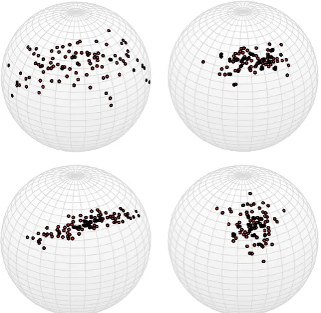
Fig. 1 Samples of 100 observations from some example ESAG

distributions with parameters (clock-wise from top left): μ = (−1,−2,2), γ = (−1,1);μ = (−2,−4,4), γ = (−1,1); μ=(−2,−4,4), γ =(0,0);μ=(−2,−4,4), γ=(−3,1)

ESAG(μ, γ ). The rotationally symmetric isotropic angular Gaussian corresponds to

V =I3⇔γ =(0,0)=0

hence we will write ESAG(μ,0)≡IAG(μ).

Remark 3 (Simulation.) To simulatey∼ESAG(μ, γ ), sim-ulatez ∼ N(μ,V)whereV = V(μ, γ )is defined in (18) then sety=z/z.

Fig. 2 Estimates of the Earth’s historic magnetic pole position; see Sect.2.5for a description of the data. (Left) shows contours of con-stant probability density for fitted models corresponding to 99, 95 and 50% coverage and (Right) shows 95% confidence regions for the mean direction calculated as described in Sect.2.4. ESAG is shown with solid blue lines and the IAG with black dotted lines

Remark 5 (Parameter orthogonality.) The parameter vectors

μandγare orthogonal, in the sense that

Iμ,γ =Iγ,μ =03,2,

where I_μ,γ = −E_μ,γ ∂2log f1/∂μ∂γ

. Moreover, the directional and magnitudinal componentsμandγ, that is, μ,μ/μ,γandγ /γ, are all mutually orthogonal. The proofs follow easily from the symmetries of fESAGand are omitted.

Often in applications, there is particular interest in the directional mean,m =μ/μ. A parametric bootstrap pro-cedure to construct confidence regions form, which exploits both the ease of simulation and the parameter orthogonality, is as follows.

2.4 Parametric bootstrap confidence regions for

m=μ/μ

Letl(μ, γ )denote the log-likelihood for a sampley1, . . . ,yn each of which is assumed to be an independent ESAG(μ, γ ) random variable and define

(μ, γ )=

−∂_∂μ∂μ2l(μ, γ )

−1

.

Denote the maximum likelihood estimate of (μ, γ ) by

(μ,ˆ γ )ˆ , let mˆ = ˆμ/|| ˆμ||,ˆ = (μ,ˆ γ )ˆ and letξˆ1 andξˆ2 denote the maximum likelihood estimates of the axes of sym-metry (15), such thatmˆ,ξˆ1andξˆ2are mutually orthogonal unit vectors. Define the matrixξˆ =(ξˆ1,ξˆ2), then test statis-tic

T(m)=mξˆ

1

|| ˆμ||2ξˆˆξˆ

₋1

ˆ

ξm, (19)

ν₁

-1 -0.5 0 0.5 1

ν 2

-0.6 -0.3 0 0.3 0.6

ESAG Kent

ESAG Kent

ν₁

density

0 0.2 0.4 0.6 0.8 1 1.2

Kent ESAG

ν₂

-1.5 -1 -0.5 0 0.5 1 1.5

-1.5 -1 -0.5 0 0.5 1 1.5

density

0 0.2 0.4 0.6 0.8 1 1.2

Kent ESAG

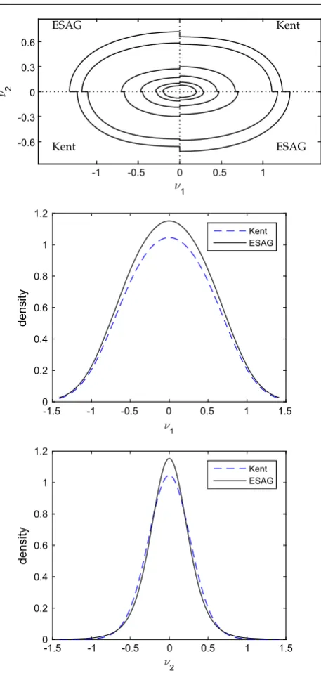
Fig. 3 A comparison of ESAG and Kent densities with parameters

matched by fitting each distribution to the same dataset; see Sect.3 for details. (Top) shows a tangent plane projection, in terms of tangent plane coordinatesν1andν2, of contours of constant probability density for coverage levels 95, 90, 50, 25, 10, 5%. (Centre) and (Bottom) show transects of the two probability density functions withν2 = 0 and ν1=0, respectively

is suitable for defining confidence regions for m as

statis-tic (19), withξ,ˆ μ,ˆ ˆ replaced by corresponding quantities calculated from the bootstrap sample; thencis the(1−α) quantile of the resulting statisticsT₁∗(mˆ), . . . ,T_B∗(mˆ). Exam-ples of confidence regions calculated by this algorithm are shown in Fig.2(right).

2.5 An example: estimates of the historic position of Earth’s magnetic pole

This dataset contains estimates of the position of the Earth’s historic magnetic pole calculated from 33 different sites in Tasmania (Schmidt 1976). The data are shown in Fig.2with contours of fitted IAG and ESAG distributions. The maxi-mum likelihood estimates of the parameters are respectively

ˆ

μ_{=(−2.18,0.94,3.06),}

and

(μˆ,γˆ)=(−2.33,1.11,3.34,0.17,−0.78).

Twice the difference in maximised log-likelihoods equals 14.12, which when referred to aχ₂2distribution (see Remark 4) corresponds to a p-value of less than 10−3, indicating strong evidence in favour of ESAG over the IAG.

3 A comparison of ESAG with the Kent

distribution

Figure3 shows contours and transects of the densities of ESAG and Kent distributions. The parameter values for each are computed by fitting the two models to a large sam-ple of independent and identically distributed data from ESAG(μ,γ), with μ = (0,0,2.5) and γ = (0.75,0). For the inner contours ESAG is more anisotropic than the matched Kent distribution and appears slightly more peaked at the mean. Besides these small differences, the figure shows that ESAG and Kent distributions are very similar distribu-tions in this example, as we have found them to be more generally. Indeed, preliminary results, not presented here, suggest that for typical sample sizes it is usually very difficult to distinguish between them using a statistical criterion. This warrants making the modelling choice between using the Kent distribution or the ESAG on grounds of practical conve-nience. The Kent distribution is a member of the exponential family, but its density involves a non-closed-form normalis-ing constant, and simulation requires a rejection algorithm (Kent et al. 2013). The ESAG distribution has a density that is less tidy than the Kent density, hence less suited to com-puting moment estimators, etc., but this is not much of a drawback given that its density can be computed exactly so that the exact likelihood can be easily maximised. Moreover,

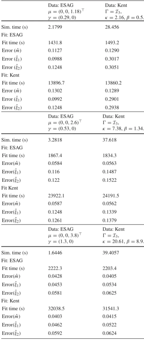
Table 1 Results of simulation study for fitting the ESAG and Kent

distributions to both ESAG and Kent simulated data

Data: ESAG Data: Kent μ=(0,0,1.18) =I3,

γ =(0.29,0) κ=2.16,β=0.5.

Sim. time (s) 2.1799 28.456

Fit: ESAG

Fit time (s) 1431.8 1493.2

Error (mˆ) 0.1127 0.1290

Error (ξˆ1) 0.0988 0.3017

Error (ξˆ2) 0.1248 0.3051

Fit: Kent

Fit time (s) 13896.7 13860.2

Error (mˆ) 0.1302 0.1289

Error (ξˆ1) 0.0992 0.2901

Error (ξˆ2) 0.1248 0.2938

Data: ESAG Data: Kent μ=(0,0,2.6) =I3,

γ =(0.53,0) κ=7.38,β=1.34.

Sim. time (s) 3.2818 37.618

Fit: ESAG

Fit time (s) 1867.4 1834.3

Error(mˆ) 0.0584 0.0563

Error(ξˆ1) 0.116 0.1487

Error(ξˆ2) 0.122 0.1522

Fit Kent

Fit time (s) 23922.1 24191.5

Error(mˆ) 0.0587 0.0562

Error(ξˆ1) 0.1248 0.1339

Error(ξˆ2) 0.1261 0.1379

Data: ESAG Data: Kent μ=(0,0,3.8) =I3,

γ =(1.3,0) κ=20.61,β=8.9.

Sim. time (s) 1.6446 39.4057

Fit: ESAG

Fit time (s) 2222.3 2203.4

Error(mˆ) 0.0428 0.0405

Error(ξˆ1) 0.0453 0.0534

Error(ξˆ2) 0.0581 0.0625

Fit: Kent

Fit time (s) 32038.5 31541.3

Error(mˆ) 0.0403 0.0415

Error(ξˆ1) 0.0462 0.0522

Error(ξˆ2) 0.0592 0.0624

The results are for three different cases, involving pairs of ESAG and Kent distributions with parameters “matched” in the sense that the were fitted to an initial common set of data. For each combination of model and parameter set, we simulatedb = 500 Monte Carlo samples of

n=100 observations. The measures of error ofmˆ,ξˆ1andξˆ2are defined in the text. Simulation times, given in seconds, are cumulative over the

simulating from ESAG is particularly quick and easy (see Remark3).

Table1shows the results of a simulation study, including computational timings, for fitting ESAG and Kent densities to ESAG and Kent simulated data. To approximate the Kent normalising constant when fitting the Kent distribution, we use a saddlepoint approximation method (seeKume et al. 2013), and for simulating from the Kent distribution, we use the rejection method ofKent et al.(2013). A notion of accu-racy of the fitted model is how well the mean direction of the fitted model,mˆ, corresponds with the population mean direction,m. A measure we use for this is

2{(1−E(mˆm)}, (20)

with the expectation approximated by Monte Carlo; hence in the tables, we report

Error(mˆ)=

₂

1−b−1 b

i=1

ˆ m_(i)m

wheremˆ₍i) is the mean direction of the fitted model for the ith run out ofbMonte Carlo runs. We also consider accuracy of the major and minor axes of the fitted model. Since the signs ofξˆ1andξˆ2are arbitrary, in this case we define

Error(ξˆ1)=

₂

1−b−1 b

i=1

ξˆ

1(i)ξ1

,

and similar forξˆ2.

Note that in interpreting the results in Table1, the differ-ent simulation times of ESAG and Kdiffer-ent should be compared across columns, whereas the fitting times and accuracies should be compared across rows.

The results show, as expected, that the accuracy ofmˆ,ξˆ1, andξˆ2is typically better when the data-generating model is fitted. However, the accuracy is not dramatically worse when the non-data-generating model is fitted, i.e., when ESAG is fitted to Kent data, or the Kent distribution is fitted to ESAG data. There is a very notable difference in computation times between ESAG and Kent: for both simulation and fitting, ESAG is typically more than an order of magnitude faster than Kent.

4 Conclusion

In the pre-computer days of statistical modelling, the Fisher– Bingham family was perhaps favoured over the angular Gaussian family on account of having a simpler density,

which makes it more amenable to constructing classical esti-mators such as moment estiesti-mators. However, in the era of computational statistics, the less simple form of the angu-lar Gaussian density is hardly a barrier and is more than compensated by having a normalising constant that is trivial to evaluate. The likelihood can consequently be computed quickly and exactly, and maximised directly. Wang and Gelfand(2013) have recently argued in favour of the gen-eral angular Gaussian distribution as a model for Bayesian analysis of circular data. For spherical data, a major obstacle to using the general angular Gaussian distribution is that its parameters are poorly identified by the data. The ESAG sub-family overcomes this problem, and is a direct analogy of the Kent subfamily of the general Fisher–Bingham distribution. Besides having a tractable likelihood, the ease and speed with which ESAG can be simulated makes it especially well suited to methods of simulation-based inference. Natural wider applications of ESAG include using it as an error distribution for spherical regression models with anisotropic errors; for classification on the sphere (as a model for class-conditional densities); and for clustering spherical data (based on ESAG mixture models). Code written in MATLAB for performing calculations in this paper is available at the second author’s web page.

Open Access This article is distributed under the terms of the Creative

Commons Attribution 4.0 International License (http://creativecomm ons.org/licenses/by/4.0/), which permits unrestricted use, distribution, and reproduction in any medium, provided you give appropriate credit to the original author(s) and the source, provide a link to the Creative Commons license, and indicate if changes were made.

A Proofs

A.1 Properties of the functionMd(α)

Integrating (3) by parts, we obtain

Md−1(α)=

d−1udφ(u−α)

_∞

u=0

+d−1

_∞

0

ud(u−α)φ(u−α)du

=d−1Md+1(α)−d−1αMd(α),

which implies that

Md+1(α)=αMd(α)+dMd−1(α). (21)

Moreover, differentiating (3) with respect toα, and exchang-ing the order of differentiation and integration on the RHS, we obtain

where a prime denotes differentiation; and, using (21) and (22) together, it is found that

Md(α)=dMd₋1(α). (23)

Further points to note, which are easily established by induc-tion, are that we can write

Md(α)=Pd(α)(d)(α)+Qd(α)φ(α),

wherePd(α)is a polynomial of orderdandQdis a polyno-mial of orderd −1; andPd(α)inherits the properties (21) and (23) ofMd(α), whileQd(α)inherits (21) but not (23); instead of (23), we haveQ_d(α)=Qd+1(α)−Pd(α). One relevant property ofPd(α)is that the coefficient of its lead-ing termαdis 1; this follows from either (21) or (23) applied repeatedly toPd(α). As an easy consequence, we obtain a result that is used below: for any fixed integerd ≥0,

Md(α)∼αd as α→ ∞. (24)

A.2 Proof of Proposition1

From (8) it follows that 1/ρd₋1≤1/ρjfor j=1, . . . ,d−2. As a consequence, we can restrict attention toyof the form y=(0, . . . ,u, (1−u2)1/2)whereu is in a neighbourhood of 0. Substituting this form ofyinto (7) and differentiating, it is seen that

∂log f1

∂u (u)

u=0

=0,

and, using (22), it is found that

∂2_{log f} 1

∂u2 (u)

u=0

=δd−α2+α2δ

+(d−1)(δ−1)αMd−2(α)/Md−1(α), (25)

whereδ =(ρd₋1−1)/ρd₋1. The pointu =0, which cor-responds toy =ξd, is a maximum or minimum depending on whether (25) is negative or positive and, using this fact, Proposition 2.1 follows after some elementary further

manip-ulations.

A.3 Proof of Proposition2

First, consider the exponent in (7). Using (9) it follows after some elementary calculations that

1 2

yμ2

yV−1_y −μμ = − 1 2α

2

d−1 j=1y2j/ρj 1+d₌−1y2/ρj

. (26)

Now define uj = αyj, j = 1, . . . ,d −1 and suppose that α → ∞ while the uj remain fixed. Then, since

d j=1

yξj

2

= 1, it follows that asα → ∞, y → 1. Consequently as theρj are remaining fixed, it is easy to see that

yV−1y→1. (27)

Moreover, from (12) it follows thatyμ∼αand therefore, from (24),

Md−1

yμ/

yV−1y

1/2

∼αd−1_.

(28)

Lettingα→ ∞and substituting (26), (27) and (28) into (7) we obtain pointwise convergence to the(d−1)-dimensional multivariate Gaussian density φd−1(u|0d−1, ) multiplied by a factorαd−1; this factor is the Jacobian of the transfor-mation from(y1, . . . ,yd−1)to(u1, . . . ,ud−1).

A.4 Proof of Lemma1

Using the standard trigonometric results cos2ψ = (1 + cos 2ψ)/2 and sin2ψ = (1−cos 2ψ)/2, and making use of the fact thatξ˜1ξ˜₁+ ˜ξ2ξ˜₂+ξ3ξ₃=I3becauseξ˜1,ξ˜2and

ξ3are mutually orthogonal unit vectors, (16) becomes

V−1=I3+1₂(ρ−1−ρ)cos 2ψ

˜

ξ1ξ˜1− ˜ξ2ξ˜2

+1 2(ρ−

1_−ρ) sin 2ψ

˜

ξ1ξ˜2+ ˜ξ2ξ˜1

+1 2(ρ−

1_+ρ− 2)

˜

ξ1ξ˜1+ ˜ξ2ξ˜2

(29)

From (17),(γ₁2+γ₂2)1/2=(ρ−1−ρ)/2, and we may solve forρto obtainρ =(1+γ₁2+γ₂2)1/2−(γ₁2+γ₂2)1/2, and with some elementary further calculation we see that

(ρ−1_{+ρ−2)/2=(1+γ}2

1 +γ22)1/2−1. (30)

Finally, substituting (17) and (30) into (29), we obtain (18).

References

Absil, P.A., Baker, C.G., Gallivan, K.A.: Trust-region methods on Rie-mannian manifolds. Found. Comput. Math.7(3), 303–330 (2007). doi:10.1007/s10208-005-0179-9

Boumal, N., Mishra, B., Absil, P.A., Sepulchre, R.: Manopt, a Matlab toolbox for optimization on manifolds. J. Mach. Learn. Res. vol. 15, pp. 1455–1459.http://www.manopt.org(2014)

Hernandez-Stumpfhauser, D., Breidt, F., van der Woerd, M.: The general projected normal distribution of arbitrary dimension: mod-eling and Bayesian inference. Bayesian Anal. 12(1), 113–133 (2017)

Kent, J.T.: The Fisher-Bingham distribution on the sphere. J. R. Stat. Soc. Series B44, 71–80 (1982)

Kent, J.T., Ganeiber, A., Mardia, K.V.: A new method to simulate the Bingham and related distributions in directional data analysis with applications. arXiv preprintarXiv:1310.8110(2013)

Kume, A., Preston, S.P., Wood, A.T.A.: Saddlepoint approximations for the normalizing constant of Fisher-Bingham distributions on prod-ucts of spheres and Stiefel manifolds. Biometrika100(4), 971–984 (2013)

Mardia, K.V.: Statistics of directional data (with discussion). J. R. Stat. Soc. Series B37, 349–393 (1975)

Mardia, K.V., Jupp, P.E.: Directional Statistics. Wiley, Hoboken (2000) Presnell, B., Morrison, S.P., Littell, R.C.: Projected multivariate linear models for directional data. J. Am. Stat. Assoc.93, 1068–1077 (1998)

Schmidt, P.: The non-uniqueness of the Australian Mesozoic palaeo-magnetic pole position. Geophys. J. Int.47(2), 285–300 (1976) Teanby, N.: An icosahedron-based method for even binning of globally

distributed remote sensing data. Comput. Geosci.32(9), 1442– 1450 (2006)