Structured Prediction via Learning to Search under Bandit Feedback
Amr Sharaf and Hal Daum´e III
University of Maryland, College Park
{amr,hal}@cs.umd.edu
Abstract
We present an algorithm for structured prediction under online bandit feedback. The learner repeatedly predicts a sequence of actions, generating a structured output. It then observes feedback for that output and no others. We consider two cases: a pure bandit setting in which it only ob-serves a loss, and more fine-grained feed-back in which it observes a loss for every action. We find that the fine-grained feed-back is necessary for strong empirical per-formance, because it allows for a robust variance-reduction strategy. We empiri-cally compare a number of different algo-rithms and exploration methods and show the efficacy of BLS on sequence labeling and dependency parsing tasks.
1 Introduction
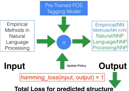
In structured prediction the goal is to jointly pre-dict the values of a collection of variables that in-teract. In the usual “supervised” setting, at train-ing time, you have access to ground truth outputs (e.g., dependency trees) on which to build a pre-dictor. We consider the substantially harder case of online bandit structured prediction, in which the system never sees supervised training data, but instead must make predictions and then only re-ceives feedback about the quality of that single prediction. The model we simulate (Figure 1) is:
1. the world reveals an input (e.g., a sentence) 2. the algorithm produces a single structured
prediction (e.g., full parse tree);
3. the world provides a loss (e.g., overall quality rating) and possibly a small amount of addi-tional feedback;
4. the algorithm updates itself
Input
Output
Pre-Trained POS Tagging Model
π
Total Loss for predicted structure
Update Policy
Empirical/NN
Methods/NNin/IN Natural/NNP Language/NNP
Processing/NNP
Empirical Methods in
Natural Language Processing
[image:1.595.309.526.226.379.2]hamming_loss(input, output) = 1
Figure 1: BLS for learning POS tagging. We learn a policy π, whose output a user sees. The user views predicted tags and provides a loss (and pos-sibly additional feedback, such as which words are labeled incorrectly). This is used to updateπ.
The goal of the system is to minimize it’s cumula-tive loss over time, using the feedback to improve itself. This introduces a fundamental exploration-versus-exploitation trade-off, in which the system must try new things in hopes that it will learn something useful, but also in which it is penalized (by high cumulative loss) for exploring too much.1
One natural question we explore in this paper is: in addition to the loss, what forms of feed-back are both easy for a user to provide and use-ful for a system to utilize? At one extreme, one can solicit no additional feedback, which makes the learning problem very difficult. We describe Bandit Learning to Search, BLS2, an approach
for improving joint predictors from different types of bandit feedback. The algorithm predicts out-puts and observes the loss of the predicted
struc-1Unlike active learning—in which the system chooses which examples it wants feedback on—in our setting the sys-tem is beholden to the human’s choice in inputs.
2Our implementation will be made freely available.
ture; but then it uses a regression strategy to es-timatecounterfactualcosts of (some) other struc-tures that it didnotpredict. This variance reduc-tion technique (§2.2) is akin to doubly-robust esti-mation in contextual bandits. The trade-off is that in order to accurately train these regressors, BLS requires per-action feedback from the user (e.g., which words were labeled incorrectly). It appears that this feedback is necessary; with out it, accu-racy degrades over time. Additionally, we con-sider several forms of exploration beyond a sim-ple-greedy strategy, including Boltzmann explo-ration and Thompson sampling (§2.4). We demon-strate the efficacy of these developments on POS tagging, syntactic chunking and dependency pars-ing (§3), in which we show improvements over both LOLS (Chang et al.,2015) and Policy Gradi-ent (Sutton et al.,1999).
2 Learning with Bandit Feedback
We operate in the learning to search framework, a family of algorithms for solving structured pre-diction problems, which essentially train apolicy to make sequence of decisions that are stitched to-gether into a final structured output. Such algo-rithms decompose a joint prediction task into a se-quence of action predictions, such as predicting the label of the next word in sequence labeling or predicting a shift/reduce action in dependency parsing3; these predictions are tied by features
and/or internal state. Algorithms in this family have recently met with success in neural networks (Bengio et al., 2015;Wiseman and Rush, 2016), though date back to models typically based on lin-ear policies (Collins and Roark,2004;Daum´e III and Marcu,2005;Xu et al.,2007;Daum´e III et al., 2009;Ross et al., 2010;Ross and Bagnell,2014; Doppa et al.,2014;Chang et al.,2015).
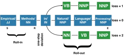
Most learning to search algorithms operate by considering a search space like that shown in Fig-ure 2. The learning algorithm first rolls-in for a few steps using aroll-in policyπin to some state
R, then considers all possible actions available at state R, and thenrolls out using aroll-out policy
πout until the end of the sequence. In the fully
supervised case, the learning algorithm can then compute a loss for all possible outputs, and use this loss to drive learning at state R, by
encourag-3Although the decomposition is into a sequence of predic-tions, such approaches are not limited to “left-to-right” style prediction tasks (Ross et al.,2010;Stoyanov et al.,2011).
in/ IN
Natural/ NNP Empirical/
JJ
Methods/ NN
Processing/ NNP Language/
NNP
VB NNP NNP
NN VB NNP
S R E
loss = 1
{
Roll-in
o
n
e
-s
te
p
d
e
v
ia
ti
o
n
{
Roll-out
loss = 0
[image:2.595.308.527.62.160.2]loss = 2
Figure 2: A search space for part of speech tag-ging, explored by a policy that chooses to “ex-plore” at state R.
ing the learner to take the action with lowest cost, updating the learned policy fromπˆitoˆπi+1.
In the bandit setting, this is not possible: we can only evaluate one loss; nevertheless, we can follow a similar algorithmic structure. Our specific algo-rithm, BLS, is summarized in algorithm 1. We start with a pre-trained reference policy πref and
seek to improve it with bandit feedback. On each example, an exploration algorithm (§2.4) chooses whether to explore or exploit. If it chooses to ex-ploit, a random learned policy is used to make a prediction and no updates are made. If, instead, it chooses to explore, it executes a roll-in as usual, a single deviation at time t according to the ex-ploration policy, and then a roll-out. Upon com-pletion it suffers a bandit loss for theentire com-plete trajectory. It then uses acost estimatorρ to guess the costs of the un-taken actions. From this it forms a complete cost vector, and updates the underlying policy based on this cost vector. Fi-nally, it updates the cost estimatorρ.
2.1 Cost Estimation by Importance Sampling
The simplest possible method of cost estimation is importance sampling (Horvitz and Thompson, 1952;Chang et al., 2015). If the third action is the one explored with probabilityp3 and a costˆc3
is observed, then the cost vector for all actions is set toh0,0,ˆc3/p3,0, . . . ,0i. This yields an
unbi-ased estimate of the true cost vector because in ex-pectation over all possible actions, the cost vector equalshcˆ1,ˆc2, . . . ,cˆKi.
Unfortunately, this type of cost estimate suffers from huge variance (see experiments in§3). If ac-tions are explored uniformly at random, then all cost vectors look like h0,0, Kcˆ3,0, . . .0i, which
exam-Input:examples{xi}Ni=1, reference policy πref, exploration algorithmexplorer,
and rollout-parameterβ ≥0
π0←initial policy
I ← ∅
ρ←initial cost estimator
foreachxiin training examplesdo
ifexplorerchooses not to explorethen
π←Unif(I)// pick policy
yi←predict usingπ
c←bandit loss ofyi
else
t←Unif(0, T−1)// deviation time
τ ←roll-in withπˆifortrounds
st←final state inτ
at=explorer(st)// deviation action
πout←πrefwith probβ, elseπˆ
i
yi←roll-out withπoutfromτ +at
c←bandit loss ofyi ˆ
c←est cost(st, τ, ρ, A(st), at, c) ˆ
πi+1 ←update(ˆπi,(Φ(xi, st),cˆ))
I ← I ∪ {πˆi+1}
update cost estimatorρ
end end
Algorithm 1:Bandit Learning to Search (BLS)
ple fromFigure 2. As in the figure, suppose that the deviation occurs at time step3and that during roll-in, the first two words are tagged correctly by the roll-in policy. Att= 3, there are 45 possible actions (each possible part of speech) to take from the deviation state, of which three are shown; each action (under uniform exploration) will be taken with probability1/45. If the first is taken, a loss of one will be observed, if the second, a loss of zero, and if the third, a loss of two. When a fair coin is flipped, perhaps the third choice is selected, which will induce a cost vector of~c = h0,0,90,0, . . .i. In expectation over this random choice, we have
Ea[c] is correct, implying unbiasedness, but the variance is very large:O((Kcmax)2).
This problem is exacerbated by the fact that many learning to search algorithms define the cost of an action a to be the difference between the cost ofaand the minimum cost. This is desirable because when the policy is predicting greedily, it should choose the action thataddsthe least cost; it should not need to account for already-incurred cost. For example, suppose the first two words in
Input:current state:st; roll-in trajectory:τ;
Kregression functions (one for every action):ρ; set of allowed actions:
A(st); roll-out policy:πout; explored action:at; bandit loss:c
t← |τ|
Initializeˆc: a vector of size|A(st)| ˆ
c0 ←0
for(a, s)∈τ do
ˆ
c0←ˆc0+ρa(Φ(s))
end
fora∈A(st)do
ifa=atthen ˆ
c(a)←c
else
ˆ
c(a)←cˆ0
y←roll-out withπout fromτ +a
for(a0, s0)inydo
ˆ
c(a)←ˆc(a) +ρa0(Φ(s0))
end end
returncˆ: a vector of size|A(st)|, wherecˆ(a) is the estimated cost for actionaat statest.
[image:3.595.317.521.62.372.2]Algorithm 2:est cost
Figure 2were tagged incorrectly. This would add a loss of2to any of the estimated costs, but could be very difficult to fit because this loss was based on past actions, not the current action.
2.2 Doubly Robust Cost Estimation
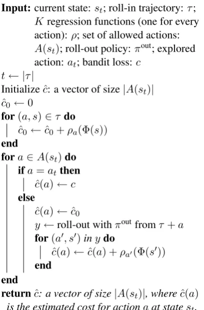
To address the challenge of high variance cost es-timates, we adopt a strategy similar to the doubly-robust estimation used in the (non-structured) con-textual bandit setting (Dudik et al.,2011). In par-ticular, we train a separate set of regressors to esti-mate the total costs of any action, which we use to impute a counterfactual cost for untaken actions.
Algorithm2spells this out, taking advantage of an action-to-cost regressor,ρ. To estimate the cost of an un-taken actiona0at a deviation, we simulate
the execution of a0, followed by the execution of
the current policy through the end. The cost of that entire trajectory is estimated by summing ρ
over all states along the path. For example, in the part of speech tagging example above, we learn 45 regressors: one for each part of speech. The cost of a roll-out is estimated as the sum of these regressors over the entire predicted sequence.
First, this is able to provide a cost estimate forall actions. Second, becauseρis deterministic, it will give the same cost to the common prefix of all tra-jectories, thus resolving credit assignment.
The remaining challenge is: how to estimate these regressors. Unfortunately, this currently comes at an additional cost to the user: we must observe per-action feedback. In particular, when the user views a predicted output (e.g., part of speech sequence), we ask for a binary signal for each action whether the predicted action was right or wrong. Thus, for a sentence of length T, we generate T training examples for every time step 1 ≤ t ≤T. Each training example has the form: (at, ct), whereatis the predicted action at timet, andctis a binary cost, either1if the predicted ac-tion was correct, or zero otherwise. This amounts to a user “crossing out” errors, which hopefully incurs low overhead. Using these T training ex-amples, we can effectively train theK regressors for estimating the cost of unobserved actions.
2.3 Theoretical Analysis
In order to analyze the variance of the BLS es-timator (in particular to demonstrate that it has lower variance than importance sampling), we provide a reduction to contextual bandits in an i.i.d setting. Dud´ık et al.(2014) studied the contextual bandit setting, which is similar to out setting but without the complexity of sequences of actions. (In particular, if T = 1 then our setting is ex-actly the contextual bandit setting.) They studied the task of off-policy evaluation and optimization for a target policyν using doubly robust estima-tion given historic data from an exploraestima-tion pol-icyµconsisting of contexts, actions, and received rewards. They prove that this approach yields ac-curate value estimates when there is either a good (but not necessarily consistent) model of rewards or a good (but not necessarily consistent) model of past policy. In particular, they show:
Theorem. Let ∆(x, a) and ρk(x, a) denote, re-spectively, the additive error of the reward esti-matorrˆand the multiplicative error of the action probability estimator µˆk. If exploration policy µ and the estimatorµˆkare stationary, and the target policyν is deterministic, then the variance of the doubly robust estimatorVµ[ ˆVDR]is:
1
n(V(x,a)∼ν[r∗(x, a) + (1−ρ1(x, a))∆(x, a)])
+E(x,a)∼νµˆ1(1a|x)ρ1(x, a)Vr∼D(·|x,a)[r]
+E(x,a)∼ν1−µˆ1(µ1(a|ax|)x)ρ1(x, a)∆(x, a)2]
The theorem show that the variance can be de-composed into three terms. The first term ac-counts for the randomness in the context features. The second term accounts for randomness in re-wards and disappears when rere-wards are determin-istic functions of the context and actions. The last term accounts for the disagreement between ac-tions taken by the exploration policy µ and the target policy ν. This decomposition shows that doubly robust estimation yields accurate value es-timates when there is either a good model of re-wards or a good model of the exploration policy.
We can build on this result for BLS to show an identicalresult under the following reduction. The exploration policyµin our setting is defined as fol-lows: for every exploration round, a randomly se-lected time-step is assigned a randomly chosen ac-tion, and a deterministic reference policy is used to generate the roll-in and roll-out trajectories. Our goal is to evaluate and optimize a better target pol-icy ν. Under this setting, and assuming that the structures are generated i.i.d from a fixed but un-known distribution, the structured prediction lem will be equivalent to a contextual bandit prob-lem were we consider the roll-in trajectory as part of the context.
2.4 Options for Exploration Strategies
In addition to the-greedy exploration algorithm, we consider the following exploration strategies:
Boltzmann (Softmax) Exploration. Boltz-mann exploration varies the action probabilities as a graded function of estimated value. The greedy action is still given the highest selection probability, but all the others are ranked and weighted according to their cost estimates; ac-tion a is chosen with probability proportional to exph 1
tempc(a)
i
Thompson Sampling estimates the following elements: a setΘof parametersµ; a prior distribu-tion P(µ)on these parameters; past observations
D consisting of observed contexts and rewards; a likelihood function P(r|b, µ), which gives the probability of reward given a contextband a pa-rameter µ; In each round, Thompson Sampling selects an action according to its posterior prob-ability of having the best parameter µ. This is achieved by taking a sample of parameter for each action, using the posterior distributions, and se-lecting that action that produces the best sam-ple (Agrawal and Goyal,2013;Komiyama et al., 2015). We use Gaussian likelihood function and Gaussian prior for the Thompson Sampling algo-rithm. In addition, we make a linear payoff as-sumption similar to (Agrawal and Goyal, 2013), where we assume that there is an unknown under-lying parameterµa ∈ Rd such that the expected cost for each actiona, given the statestand con-textxiisΦ(xi, st)Tµa.
3 Experimental Results
The evaluation framework we consider is the fully online setup described in the introduction, mea-suring the degree to which various algorithms can effectively improve upon a reference policy by ob-serving only a partial feedback signal, and effec-tively balancing exploration and exploitation. We learn from one structured example at every time step, and we do a single pass over the available examples. We measure loss as the average cumu-lative loss over time, thus algorithms are appropri-ately “penalized” for unnecessary exploration.
3.1 Tasks, Policy Classes and Data Sets
We experiment with the following three tasks. For each, we briefly define the problem, describe the policy class that we use for solving that problem in a learning to search framework (we adopt a sim-ilar setting to that of (Chang et al.,2016), who de-scribes the policies in more detail), and describe the data sets that we use. The regression problems are solved using squared error regression, and the classification problems (policy learning) is solved via cost-sensitive one-against-all.
Part-Of-Speech Tagging over the 45 Penn Treebank (Marcus et al., 1993) tags. To simu-late a domain adaptation setting, we train a ref-erence policy on the TweetNLP dataset (Owoputi et al.,2013), which achieves good accuracy in
do-main, but does poorly out of domain. We sim-ulate bandit feedback over the entire Penn Tree-bank Wall Street Journal (sections 02–21 and 23), comprising42k sentences and about one million words. (AdaptingfromtweetstoWSJ is nonstan-dard; we do it here because we need a large dataset on which to simulate bandit feedback.) The mea-sure of performance is average per-word accuracy (one minus Hamming loss).
Noun Phrase Chunkingis a sequence segmen-tation task, in which sentences are divided into base noun phrases.We solve this problem using a sequence span identification predictor based on Begin-In-Out encoding, following (Ratinov and Roth, 2009), though applied to chunking rather than named-entity recognition. We used the CoNLL-2000 datasetfor training and testing. We used the smaller test split (2,012 sentences) for training a reference policy, and used the training split (8,500sentences) for online evaluation. Per-formance was measured by F-score over predicted noun phrases (for which one has to predict the en-tire noun phrase correctly to get any points).
Dependency Parsing is a syntactic analysis task, in which each word in a sentence gets as-signed a grammatical head (or “parent”). The ex-perimental setup is similar to part-of-speech tag-ging. We train an arc-eager dependency parser (Nivre, 2003), which chooses among (at most) four actions at each state: Shift, Reduce, Left or Right. As in part of speech tagging, the reference policy is trained on the TweetNLP dataset (us-ing an oracle due to (Goldberg and Nivre,2013)), and evaluated on the Penn Treebank corpus (again, sections02−21and section23). The loss is un-labeled attachment score (UAS), which measures the fraction of words that pick the correct parent.
3.2 Main Results
super-POS DepPar Chunk Algorithm Variant Acc UAS F-Scr A.Reference - 47.24 44.15 74.73 B.LOLS -greedy 2.29 18.55 31.76 C.BLS -greedy 86.55 56.04 90.03
D. Boltz. 89.62 57.20 90.91
E. Thomp. 89.37 56.60 90.06
F. Oracle 89.23 56.60 90.58
G.Policy∇ -greedy 75.10 - 90.07 H.DAgger Full Sup 96.51 90.64 95.29 Table 1: Total progressive accuracies for the dif-ferent algorithms on the three natural language processing tasks. LOLS uniformlydecreases per-formance over the Reference baseline. BLS, which integrates cost regressors, uniformly im-proves, often quite dramatically. The overall ef-fect of the exploration mechanism is small, but in all cases Boltzmann exploration is statistically significantly better than the other options at the
p < 0.05 level (because the sample size is so large). Policy Gradient for dependency parsing is missing because after processing 14 of the data, it was substantially subpar.
vised “upper bound” trained with DAgger. From these results, we draw the following con-clusions (the rest of this section elaborates on these conclusions in more detail):
1. The original LOLS algorithm is ineffective at improving the accuracy of a poor reference policy (A vs B);
2. Collecting additional per-word feedback in BLS allows the algorithm to drastically im-prove on the reference (A vs C) and on LOLS (B vs C); we show in§3.3that this happens because of variance reduction;
3. Additional leverage can be gained by varying the exploration strategy, and in general Boltz-mann exploration is effective (C,D,E), but the Oracle exploration strategy isnotoptimal (F vs D); see§3.4;
4. For large action spaces like POS tagging, the BLS-type updates outperform Policy Gradient-type updates, when the exploration strategy is held constant (G vs D), see§3.5. 5. Bandit feedback is less effective than full
feedback (H vs D) (§3.6).
3.3 Effect of Variance Reduction
Table 1 shows the progressive validation accura-cies for all three tasks for a variety of
algorith-0 10000 20000 30000 40000
Number of Sequences 0
10 20 30 40 50 60 70 80
Variance
BLS LOLS
[image:6.595.80.284.64.192.2]Variance for Doubly Robust and Importance Sampling
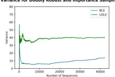
Figure 3: Analyzing the variance of the the cost estimates from LOLS and BLS over a run of the algorithm for POS; the x-axis is number of sen-tences processed, y-axis is empirical variance.
mic settings. To understand the effect of vari-ance, it is enough to compare the performance of the Reference policy (the policy learned from the out of domain data) with that of LOLS. In all of these cases, running LOLS substantially de-creases performance. Accuracy drops by 45% for POS tagging, 26% for dependency parsing and 43% for noun phrase chunking. For POS tagging, the LOLS accuracy falls belowthe accuracy one would get for random guessing (which is approxi-mately 14% on this dataset forNN)!
When the underlying algorithm changes from LOLS to BLS, the overall accuracies go up signif-icantly. Part of speech tagging accuracy increases from 47% to 86%; dependency parsing accuracy from 44% to 57%; and chunking F-score from 74% to 90%. These numbers naturally fall be-low state of the art for fully supervised learning on these data sets, precisely because these results are based only on bandit feedback (see§3.6).
3.4 Effect of Exploration Strategy
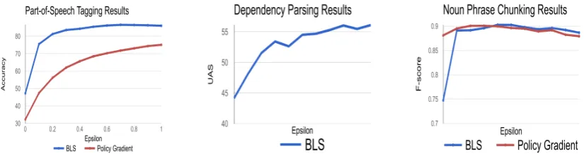
Figure 4 shows the effect of the choice of for
-greedy exploration in BLS. Overall, best results are achieved withremarkablyhigh epsilon, which is possibly counter-intuitive. The reason this hap-pens is because BLS only explores on one out ofT
[image:6.595.315.508.68.196.2]Figure 4: Analyzing the effect ofin exploration/exploitation trade-off. Overall, large values ofare strongly preferred.
Returning toTable 1, we can consider the effect of different exploration mechanisms: -greedy, Boltzmann (or softmax) exploration, and Thomp-son sampling. Overall, Boltzmann exploration was the most effective strategy, gaining about 3% accuracy in POS tagging, just over 1% in depen-dency parsing, and just shy of 1% in noun phrase chunking. Although the latter two effects are small, they are statistically significant, which is measurable due to the fact that the evaluation sets are very large. In general, Thompson sampling is also effective, though worse than Boltzmann.
Finally, we consider a variant in which when-ever BLS requests exploration, the algorithm “cheats” and chooses the gold standard decision at that point. This is the “oracle exploration” line in Table 1. We see that this does not improve overall quality, which suggests that a good explo-ration strategy is not one that always does the right thing, but one that also explored bad—but useful-to-learn-from—options.
3.5 Policy Gradient Updates
A natural question is: how does bandit structured prediction compare to more standard approaches to reinforcement learning (we revisit the question of how these problems differ in §4). We chose Policy Gradient (Sutton et al.,1999) as a point of comparison. The main question we seek to ad-dress is how the BLS update rule compares to the Policy Gradient update rule. In order to perform this comparison, we hold the exploration strategy fixed, and implement the Policy Gradient update rule inside our system.
More formally, the policy gradient optimiza-tion is similar to that used in BLS. PG maintains a policy πθ, which is parameterized by a set of parameters θ. Features are extracted from each statestto construct the feature vectorsφ(st), and
linear function approximation models the proba-bility of selecting action at at state st under πθ:
πθ(at|st) ∝ exp(θaTtφ(st)), whereK is the total
number of actions. PG maximizes the total ex-pected return under the distribution of trajectories sampled from the policyπθ.
To balance the exploration / exploitation trade-off, we use exactly the same epsilon greedy tech-nique used in BLS (Algorithm1). For each tra-jectoryτ sampled fromπθ, a state is selected uni-formly at random, and an action is selected greed-ily with probability. The policyπθis used to con-struct the roll-in and roll-out trajectories. For ev-ery trajectoryτ, we collect the same binary grades from the user as in BLS, and use them to train a re-gression function to estimate the per-step reward. These estimates are then be summed up to com-pute the total returnGtfrom time steptonwards (Algorithm2).
We use standard policy gradient update for opti-mizing the policyθbased on the observed rewards:
θ←θ+α∇θlog(πθ(st, at))Gt (1)
The results of this experiment are shown in line G ofTable 1. Here, we see that on POS tagging, where the number of actions is very large, PG sig-nificantly underperforms BLS. Our initial experi-ments in dependency parsing showed the PG sig-nificantly underperformed BLS after processing1 4
of the data. The difference is substantially smaller in chunking, where PG is on part with BLS with
-greedy exploration. Figure 4 shows the effect ofon PG, where we see that it also prefers large values of, but its performance saturates as→1.
3.6 Bandit Feedback vs Full Feedback
this comparison, we run the fully supervised al-gorithm DAgger (Ross et al., 2010) which is ef-fectively the same algorithm as LOLS and BLS under full supervision. In Table 1, we can see that full supervision dramatically improves perfor-mance from around 90% to 97% in POS tagging, 57% to 91% in dependency parsing, and 91% to 95% in chunking. Of course, achieving this im-proved performance comes at a high labeling cost: a human has to provide exact labels for each deci-sion, not just binary “yes/no” labels.
4 Discussion & Conclusion
The most similar algorithm to ours is the bandit version of LOLS (Chang et al.,2015) (which is an-alyzed theoretically but not empirically); the key differences between BLS and LOLS are: (a) BLS employs a doubly-robust estimator for “guessing” the costs of counterfactual actions; (b) BLS em-ploys alternative exploration strategies; (c) BLS is effective in practice at improving the performance of an initial policy.
In the NLP community,Sokolov et al. (2016a) andSokolov et al. (2016b) have proposed a pol-icy gradient-like method for optimizing log-linear models like conditional random fields (Lafferty et al., 2001) under bandit feedback. Their eval-uation is most impressive on the problem of do-main adaptation of a machine translation system, in which they show that their approach is able to learn solely from bandit-style feedback, though re-quiring a large number of samples.
In the learning-to-search setting, the difference betweenstructured prediction under bandit feed-back and reinforcement learning gets blurry. A distinction in the problem definition is that the world is typically assumed to be fixed and stochas-tic in RL, while the world is both determinisstochas-tic andknown(conditioned on the input, which is ran-dom) in bandit structured prediction: given a state and action, the algorithm always knows what the next state will be. A difference in solution is that there has been relatively little work in reinforce-ment learning that explicitly begins with a refer-ence policy to improve and often assumes an ab initio training regime. In practice, in large state spaces, this makes the problem almost impossi-ble, and practical settings like AlphaGo (Silver et al.,2016) require imitation learning to initialize a good policy, after which reinforcement learning is used to improve that policy.
Learning from partial feedback has generated a vast amount of work in the literature, dating back to the seminal introduction of multi-armed bandits by (Robbins,1985). However, the vast number of papers on this topic does not consider joint pre-diction tasks; see (Auer et al.,2002;Auer,2003; Langford and Zhang, 2008;Srinivas et al.,2009; Li et al., 2010; Beygelzimer et al., 2010;Dudik et al., 2011;Chapelle and Li,2011;Valko et al., 2013) and referencesinter alia. There, the system observes (bandit) feedback for every decision.
Other forms of contextual bandits on structured problems have been considered recently. Kalai and Vempala(2005) studied the structured prob-lem of online shortest paths, where one has a di-rected graph and a fixed pair of nodes(s, t). Each period, one has to pick a path fromstot, and then the times on all the edges are revealed. The goal of the learner is to improve it’s path predictions over time. Relatedly,Krishnamurthy et al.(2015) studied a variant of the contextual bandit problem, where on each round, the learner plays a sequence of actions, receives a score for each individual ac-tion, and obtains a final reward that is a linear com-bination to those scores.
In this paper, we presented a computationally efficient algorithm for structured contextual ban-dits, BLS, by combining: locally optimal learning to search (to control the structure of exploration) and doubly robust cost estimation (to control the variance of the cost estimation). This provides the first practically applicable learning to search algo-rithm for learning from bandit feedback. Unfortu-nately, this comes at a cost to the user: they must make more fine-grained judgments of correctness than in a full bandit setting. In particular, they must mark each decision as correct or incorrect:it is an open question whether this feedback can be removed without incurring a substantially larger sample complexity. A second large open question is whether the time step at which to deviate can be chosen more intelligently, similar to selective sampling (Shi et al.,2015), using active learning.
Acknowledgements
References
Shipra Agrawal and Navin Goyal. 2013. Thompson sampling for contextual bandits with linear payoffs.
InICML (3). pages 127–135.
Peter Auer. 2003. Using confidence bounds for exploitation-exploration trade-offs. The Journal of
Machine Learning Research3:397–422.
Peter Auer, Nicolo Cesa-Bianchi, Yoav Freund, and Robert E Schapire. 2002. The nonstochastic multi-armed bandit problem.SIAM Journal on Computing
32(1):48–77.
Samy Bengio, Oriol Vinyals, Navdeep Jaitly, and Noam Shazeer. 2015. Scheduled sampling for se-quence prediction with recurrent neural networks.
InAdvances in Neural Information Processing
Sys-tems. pages 1171–1179.
Alina Beygelzimer, John Langford, Lihong Li, Lev Reyzin, and Robert E Schapire. 2010. Contextual bandit algorithms with supervised learning guaran-tees. arXiv preprint arXiv:1002.4058.
Kai-Wei Chang, He He, Hal Daum´e III, John Langford, and St´ephane Ross. 2016. A credit assignment com-piler for joint prediction. InNIPS.
Kai-Wei Chang, Akshay Krishnamurthy, Alekh Agar-wal, Hal Daum´e III, and John Langford. 2015. Learning to search better than your teacher. In Pro-ceedings of The 32nd International Conference on
Machine Learning. pages 2058–2066.
Olivier Chapelle and Lihong Li. 2011. An empirical evaluation of thompson sampling. In Advances in
neural information processing systems. pages 2249–
2257.
Michael Collins and Brian Roark. 2004. Incremental parsing with the perceptron algorithm. In Proceed-ings of the 42nd Annual Meeting on Association for
Computational Linguistics. Association for
Compu-tational Linguistics, page 111.
Hal Daum´e III, John Langford, and Daniel Marcu. 2009. Search-based structured prediction. Machine
learning75(3):297–325.
Hal Daum´e III and Daniel Marcu. 2005. Learning as search optimization: Approximate large margin methods for structured prediction. InProceedings of the 22nd international conference on Machine
learning. ACM, pages 169–176.
Janardhan Rao Doppa, Alan Fern, and Prasad Tade-palli. 2014. Hc-search: A learning framework for search-based structured prediction. J. Artif. Intell.
Res.(JAIR)50:369–407.
Miroslav Dud´ık, Dumitru Erhan, John Langford, Li-hong Li, et al. 2014. Doubly robust policy evaluation and optimization. Statistical Science
29(4):485–511.
Miroslav Dudik, Daniel Hsu, Satyen Kale, Nikos Karampatziakis, John Langford, Lev Reyzin, and Tong Zhang. 2011. Efficient optimal learning for contextual bandits. arXiv preprint arXiv:1106.2369
.
Yoav Goldberg and Joakim Nivre. 2013. Training de-terministic parsers with non-dede-terministic oracles.
Transactions of the ACL1.
Daniel G Horvitz and Donovan J Thompson. 1952. A generalization of sampling without replacement from a finite universe. Journal of the American
sta-tistical Association47(260):663–685.
Adam Kalai and Santosh Vempala. 2005. Efficient al-gorithms for online decision problems. Journal of
Computer and System Sciences71(3):291–307.
Junpei Komiyama, Junya Honda, and Hiroshi Nak-agawa. 2015. Optimal regret analysis of thomp-son sampling in stochastic multi-armed bandit problem with multiple plays. arXiv preprint
arXiv:1506.00779.
Akshay Krishnamurthy, Alekh Agarwal, and Miroslav Dudik. 2015. Efficient contextual semi-bandit
learn-ing.arXiv preprint arXiv:1502.05890.
John Lafferty, Andrew McCallum, and Fernando CN Pereira. 2001. Conditional random fields: Prob-abilistic models for segmenting and labeling se-quence data .
John Langford and Tong Zhang. 2008. The epoch-greedy algorithm for multi-armed bandits with side information. InAdvances in neural information
pro-cessing systems. pages 817–824.
Lihong Li, Wei Chu, John Langford, and Robert E Schapire. 2010. A contextual-bandit approach to personalized news article recommendation. In Pro-ceedings of the 19th international conference on
World wide web. ACM, pages 661–670.
Mitchell P Marcus, Mary Ann Marcinkiewicz, and Beatrice Santorini. 1993. Building a large annotated corpus of english: The penn treebank.
Computa-tional linguistics19(2):313–330.
Joakim Nivre. 2003. An efficient algorithm for projec-tive dependency parsing. InIWPT. pages 149–160. Olutobi Owoputi, Brendan O’Connor, Chris Dyer,
Kevin Gimpel, Nathan Schneider, and Noah A Smith. 2013. Improved part-of-speech tagging for online conversational text with word clusters. Asso-ciation for Computational Linguistics.
Lev Ratinov and Dan Roth. 2009. Design challenges and misconceptions in named entity recognition. In
CoNLL.
Herbert Robbins. 1985. Some aspects of the sequential design of experiments. InHerbert Robbins Selected
Stephane Ross and J Andrew Bagnell. 2014. Rein-forcement and imitation learning via interactive no-regret learning. arXiv preprint arXiv:1406.5979. St´ephane Ross, Geoffrey J Gordon, and J Andrew
Bag-nell. 2010. A reduction of imitation learning and structured prediction to no-regret online learning.
arXiv preprint arXiv:1011.0686.
Tianlin Shi, Jacob Steinhardt, and Percy Liang. 2015. Learning where to sample in structured prediction.
InAISTATS.
David Silver, Aja Huang, Chris J Maddison, Arthur Guez, Laurent Sifre, George Van Den Driessche, Ju-lian Schrittwieser, Ioannis Antonoglou, Veda Pan-neershelvam, Marc Lanctot, et al. 2016. Mastering the game of go with deep neural networks and tree search. Nature529(7587):484–489.
Artem Sokolov, Julia Kreutzer, Christopher Lo, and Stefan Riezler. 2016a. Learning structured predic-tors from bandit feedback for interactive NLP. In
Proceedings of the 54th Annual Meeting of the As-sociation for Computational Linguistics (Volume 1:
Long Papers). Association for Computational
Lin-guistics (ACL). https://doi.org/10.18653/v1/p16-1152.
Artem Sokolov, Stefan Riezler, and Tanguy Urvoy. 2016b. Bandit structured prediction for learning from partial feedback in statistical machine transla-tion. arXiv preprint arXiv:1601.04468.
Niranjan Srinivas, Andreas Krause, Sham M Kakade, and Matthias Seeger. 2009. Gaussian process opti-mization in the bandit setting: No regret and experi-mental design. arXiv preprint arXiv:0912.3995. Veselin Stoyanov, Alexander Ropson, and Jason
Eis-ner. 2011. Empirical risk minimization of graphi-cal model parameters given approximate inference, decoding, and model structure. InAISTATS. pages 725–733.
Richard S Sutton, David A McAllester, Satinder P Singh, Yishay Mansour, et al. 1999. Policy gradient methods for reinforcement learning with function approximation. In NIPS. volume 99, pages 1057– 1063.
Michal Valko, Nathaniel Korda, R´emi Munos, Ilias Flaounas, and Nelo Cristianini. 2013. Finite-time analysis of kernelised contextual bandits. arXiv
preprint arXiv:1309.6869.
Sam Wiseman and Alexander M Rush. 2016. Sequence-to-sequence learning as beam-search op-timization. arXiv preprint arXiv:1606.02960. Yuehua Xu, Alan Fern, and Sung Wook Yoon. 2007.