Learning Composition Models for Phrase Embeddings

Learning Composition Models for Phrase Embeddings

Mo Yu Machine Intelligence

& Translation Lab Harbin Institute of Technology

Harbin, China [email protected]

Mark Dredze

Human Language Technology Center of Excellence Center for Language and Speech Processing

Johns Hopkins University Baltimore, MD, 21218 [email protected]

Abstract

Lexical embeddings can serve as useful rep-resentations for words for a variety of NLP tasks, but learning embeddings for phrases can be challenging. While separate embeddings are learned for each word, this is infeasible for every phrase. We construct phrase em-beddings by learning how to compose word embeddings using features that capture phrase structure and context. We propose efficient unsupervised and task-specific learning objec-tives that scale our model to large datasets. We demonstrate improvements on both language modeling and several phrase semantic simi-larity tasks with various phrase lengths. We make the implementation of our model and the datasets available for general use.

1 Introduction

Word embeddings learned by neural language mod-els (Bengio et al., 2003; Collobert and Weston, 2008; Mikolov et al., 2013b) have been success-fully applied to a range of tasks, including syn-tax (Collobert and Weston, 2008; Turian et al., 2010; Collobert, 2011) and semantics (Huang et al., 2012; Socher et al., 2013b; Hermann et al., 2014). However, phrases are critical for capturing lexical meaning for many tasks. For example, Collobert and Weston (2008) showed that word embeddings yielded state-of-the-art systems on word-oriented tasks (POS, NER) but performance on phrase ori-ented tasks, such as SRL, lags behind.

We propose a new method for compositional se-mantics that learns to compose word embeddings

into phrases. In contrast to a common approach to phrase embeddings that uses pre-defined compo-sition operators (Mitchell and Lapata, 2008), e.g., component-wise sum/multiplication, we learn com-position functions that rely on phrase structure and context. Other work on learning compositions relies on matrices/tensors as transformations (Socher et al., 2011; Socher et al., 2013a; Hermann and Blun-som, 2013; Baroni and Zamparelli, 2010; Socher et al., 2012; Grefenstette et al., 2013). However, this work suffers from two primary disadvantages. First, these methods have high computational complexity for dense embeddings:O(d2)orO(d3)for compos-ing every two components withddimensions. The high computational complexity restricts these meth-ods to use very low-dimensional embeddings (25 or 50). While low-dimensional embeddings perform well for syntax (Socher et al., 2013a) and sentiment (Socher et al., 2013b) tasks, they do poorly on se-mantic tasks. Second, because of the complexity, they use supervised training with small task-specific datasets. An exception is the unsupervised objec-tive of recursive auto-encoders (Socher et al., 2011). Yet this work cannot utilize contextual features of phrases and still poses scaling challenges.

In this work we propose a novel compositional transformation called the Feature-rich Composi-tional Transformation (FCT) model. FCT produces phrases from their word components. In contrast to previous work, our approach to phrase composi-tion can efficiently utilize high dimensional embed-dings (e.g.d= 200) with an unsupervised objective, both of which are critical to doing well on seman-tics tasks. Our composition function is

parameter-227

ized to allow the inclusion of features based on the phrase structure and contextual information, includ-ing positional indicators of the word components. The phrase composition is a weighted summation of embeddings of component words, where the sum-mation weights are defined by the features, which allows for fast composition.

We discuss a range of training settings for FCT. For tasks with labeled data, we utilize task-specific training. We begin with embeddings trained on raw text and then learn compositional phrase parameters as well as fine-tune the embeddings for the specific task’s objective. For tasks with unlabeled data (e.g. most semantic tasks) we can train on a large corpus of unlabeled data. For tasks with both labeled and unlabeled data, we consider a joint training scheme. Our model’s efficiency ensures we can incorporate large amounts of unlabeled data, which helps miti-gate over-fitting and increases vocabulary coverage. We begin with a presentation ofFCT(§2), includ-ing our proposed features for the model. We then present three training settings (§3) that cover lan-guage modeling (unsupervised), task-specific train-ing (supervised), and joint (semi-supervised) set-tings. The remainder of the paper is devoted to eval-uation of each of these settings.

2 Feature-rich Compositional

Transformations from Words to Phrases We learn transformations for composing phrase em-beddings from the component words based on ex-tracted features from a phrase, where we assume that the phrase boundaries are given. The result-ing phrase embeddresult-ing is based on a per-dimension weighted average of the component phrases. Con-sider the example of base noun phrases (NP), a com-mon phrase type which we want to compose. Base NPs often have flat structures – all words modify the head noun – which means that our transformation should favor the head noun in the composed phrase embedding. For each of theN wordswiin phrasep

we construct the embedding:

ep= N

X

i

λiewi (1)

whereewi is the embedding for wordi; andrefers

to point-wise product. λi is a weight vector that is

constructed based on the features ofpand the model parameters:

λij =

X

k

αjkfk(wi, p) +bij (2)

wherefk(wi, p) is a feature function that considers

word wi in phrase p and bij is a bias term. This

model is fast to train since it has only linear transfor-mations: the only operations are vector summation and inner product. Therefore, we learn the model parametersαtogether with the embeddings. We call this the Feature-rich Compositional Transformation (FCT) model.

Consider some example phrases and associated features. The phrase “the museum” should have an embedding nearly identical to “museum” since “the” has minimal impact the phrase’s meaning. This can be captured through part-of-speech (POS) tags, where a tag of DT on “the” will lead to λi ≈ ~0,

removing its impact on the phrase embedding. In some cases, words will have specific behaviors. In the phrase “historic museum”, the word “historic” should impact the phrase embedding to be closer to “landmark”. To capture this behavior we add smoothed lexical features, where smoothing reduces data sparsity effects. These features can be based on word clusters, themselves induced from pre-trained word embeddings.

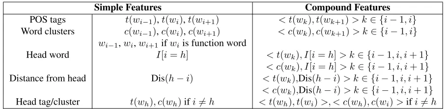
Our feature templates are shown in Table 1. Phrase boundaries, tags and heads are identified us-ing existus-ing parsers or from Annotated Gigaword (Napoles et al., 2012) as described in Section 5. In Eq. (1), we do not limit phrase structure though the features in Table 1 tend to assume a flat structure. However, with additional features the model could handle longer phrases with hierarchical structures, and adding these features does not change our model or training objectives. Following the semantic tasks used for evaluation we experimented with base NPs (including both bigram NPs and longer ones). We leave explorations of features for complex structures to future work.

FCT has two sets of parameters: one is the fea-ture weights (α,b), the other is word embeddings

(ew). We could directly use the word embeddings

Simple Features Compound Features

POS tags t(wi−1),t(wi),t(wi+1) < t(wk), t(wk+1)> k∈ {i−1, i} Word clusters c(wi−1),c(wi),c(wi+1) < c(wk), c(wk+1)> k∈ {i−1, i}

wi−1,wi,wi+1ifwiis function word

Head word I[i=h] < t(wk), I[i=h]> k∈ {i−1, i, i+ 1}

< c(wk), I[i=h]> k∈ {i−1, i, i+ 1}

Distance from head Dis(h₋i) < t(wk),Dis(h−i)> k∈ {i−1, i, i+ 1}

< c(wk),Dis(h−i)> k∈ {i−1, i, i+ 1}

Head tag/cluster t(wh), c(wh)ifi6=h < t(wh), t(wi)>, < c(wh), c(wi)>ifi6=h

Table 1: Feature templates for wordwiin phrasep. t(w): POS tag;c(w): word cluster (when w is a function word,

i.e. a preposition word or conjunction word, there is no need to have smoothed version of the word features based on clusters. Therefore we directly use the word forms as features as shown in line 3 of the table);h: position of head word of the phrasep; Dis(i−j): distance betweenwiandwj(distance in tokens).< f1, f2>refers to the conjunction (i.e.

Cartesian product) between two feature templatesf1andf2.

learn both the feature weights and the word embed-dings with objectives in Section 3. Moreover, ex-periments show that starting with the baseline word embeddings leads to better learning results compar-ing to random initializations. Therefore in the rest of the paper, if not specifically mentioned, we always initialize the embeddings ofFCTwith baseline word embeddings learned by Mikolov et al. (2013b).

3 Training Objectives

The speed and flexibility of FCT enables a range of training settings. We consider standard unsu-pervised training (language modeling), task-specific training and joint objectives.

3.1 Language Modeling

For unsupervised training on large scale raw texts (language modeling) we trainFCTso that phrase em-beddings – as composed in Section 2 – predict con-textual words, an extension of the skip-gram objec-tive (Mikolov et al., 2013b) to phrases. For each phrasepi = (wi1, ..., win) ∈ P, wij ∈V, whereP

is the set of all phrases andV is the word vocabu-lary. Hereiis the index of a phrase in setP andij

is the absolute index of thejth component word of pi in the sentence. For predicting thecwords to the

left and right the skip-gram objective becomes:

max

α,b,ew,e0w

1 |P|

|P|

X

i=1



 X

0<j≤c

logPe0_wi

1−j|epi

+ X

0<j≤c

logPe0_win+j|epi



,

whereP(e0_w|epi) =

expe0_wTepi

P

w0_∈V exp

e0_w0Tepi

, (3)

where α,b,ew are parameters (the word

embed-dingsewbecome parameters when fine-tuning is

en-abled) ofFCTmodel defined in Section 2. As is com-mon practice, when predicting the context words we use a second set of embeddingse0_wcalledoutput em-beddings (Mikolov et al., 2013b). During training FCT parameters (α,b) and word embeddings (ew

and e0_w) are updated via back-propagation. epi is

the phrase embedding defined in Eq. (1). wi1−j is

thej-th word before phrasepi andwin+j is thej-th

word afterpi. We can use negative sampling based

Noise Contrastive Estimation (NCE) or hierarchical softmax training (HS) in (Mikolov et al., 2013b) to deal with the large output space. We refer to this objective as thelanguage modeling(LM) objective.

3.2 Task-specific Training

When we have a task for which we want to learn embeddings, we can utilize task-specific training of the model parameters. Consider the case where we wish to use phrase embeddings produced byFCTin a classification task, where the goal is to determine whether a phrasepsis semantically similar to a

can-didate phrase (or word)pi. For a phrasepsand a set

of candidate phrases{pi, yi}N1 ,yi= 1indicates

we use a classification objective:

max

α,b,ew

X

ps

N

X

i=1

yilogP(yi = 1|ps, pi)

= max

α,b,ew

X

ps

N

X

i=1

yilog

exp epsTepi

PN

j exp epsTepj

. (4)

where ep is the phrase embedding from Eq. (1).

When a candidate phrasepi is a single word, a

lex-ical embedding can be used directly to derive epi.

WhenN = 1 for eachps, i.e., we are working on

binary classification problems, the objective will re-duce to logistic loss and a biasbwill be added. For very large sets, e.g., the whole vocabulary, we use NCE to approximate the objective. We call Eq. (4) thetask-specific(TASK-SPEC) objective.

In addition to updating only theFCTparameters, we can update the embeddings themselves to im-prove the task-specific objective. We use the fine-tuning strategy (Collobert and Weston, 2008; Socher et al., 2013a) for learning task-specific word embed-dings, first training FCT and the embeddings with theLMobjective and then fine-tuning the word em-beddings using labeled data for the target task. We refer to this process as “fine-tuning word emb” in the experiment session. Note that fine tuning can be also applied to baseline word embeddings trained with the TASK-SPECobjective or the LM objective above.

3.3 Joint Training

While labeled data is the most helpful for train-ing FCT for a task, relying on labeled data alone will yield limited improvements: labeled data has low coverage of the vocabulary, which can lead to over-fitting when we updateFCTmodel parameters Eq. (4) and fine-tune word embeddings. In particu-lar, the effects of fine-tuning word embeddings are usually limited in NLP applications. In contrast to other applications, like vision, where a single input can cover most or all of the model parameters, word embeddings are unique to each word, so a word will have its embedding updated only when the word ap-pears in a training instance. As a result, only words that appear in the labeled data will benefit from fine-tuning and, by changing only part of the embedding space, the performance may be worse overall.

Language modeling provides a method to update all embeddings based on a large unlabeled corpus. Therefore, we combine the language modeling ob-ject (Eq. (3)) and the task-specific obob-ject (Eq. (4)) to yield a joint objective. When a word’s embedding is changed in a task-specific way, it will impact the rest of the embedding space through the LM objective. Thus, all words can benefit from the task-specific training.

We call this the joint objective and call the re-sulted modelFCT-Joint (FCT-Jfor short), since it up-dates the embeddings with both theLM and TASK-SPECobjectives.

In addition to jointly training both objectives, we can create a pipeline. First, we trainFCTwith theLM objective. We then fine-tune all the parameters with the TASK-SPECobjective. We call thisFCT-Pipeline (FCT-Pfor short).

3.4 Applications to Other Phrase Composition Models

While our focus is the training of FCT, we note that the above training objectives can be applied to other composition models as well. As an example, consider a recursive neural network (RNN) (Socher et al., 2011; Socher et al., 2013a), which recur-sively computes phrase embeddings based on the bi-nary sub-tree associated with the phrase with matrix transformations. For the bigram phrases considered in the evaluation tasks, suppose we are given phrase p= (w1, w2). The model then computes the phrase embeddingep as:

ep =σ(W ·[ew1 :ew2]), (5)

where[ew1 : ew2]is the concatenation of two

em-bedding vectors. W is a matrix of parameters to be learned, which can be further refined according to the labels of the children. Back-propagation can be used to update the parameter matrixW and the word embeddings during training. It is possible to train the RNN parameters W with our TASK-SPEC or LM objective: given syntactic trees, we can use RNN(instead ofFCT) to compute phrase embeddings ep, which can be used to compute the objective, and

while we can trainRNNs using small amounts of la-beled data, it is impractical to scale it to large cor-pora (i.e.LMtraining). In contrast,FCTeasily scales to large corpora.

Remark (comparison between FCT and RNN):

Besides efficiency, our FCT is also expressive. A common approach to composition, a weighted sum of the embeddings (which we include in our experi-ments asWeighted SUM), is a special case ofFCT with no non-lexical features, and a special case of RNN if we restrict the W matrix of RNN to be di-agonal. Therefore, RNN and FCT can be viewed as two different ways of improving the expressive strength of Weighted SUM. The RNNs increase expressiveness by making the transformation a full matrix (more complex but less efficient), which does not introduce any interaction between one word and its contexts.1 _{On the other hand, FCTcan make the} transformation for one word depend on its context words by extracting relevant features, while keeping the model linear.

As supported by the experimental results, our method for increasing expressiveness is more effec-tive, because the contextual information is critical for phrase compositions. By comparison, the ma-trix transformations in RNNs may be unnecessarily complicated and are not significantly more helpful in modeling the target tasks and make the models more likely to over-fit.

4 Parameter Estimation

Training of FCT can be easily accomplished by stochastic gradient descent (SGD). While SGD is fast, training with the LM or joint objectives re-quires the learning algorithm to scale to large cor-pora, which can be slow even for SGD.

Asynchronous SGD for FCT: We use the dis-tributed asynchronous SGD-based algorithm from Mikolov et al. (2013b). The shared embeddings are updated by each thread based on training data within the thread independently. With word embeddings, the collision rate is low since it is unlikely that dif-ferent threads will update the same word at the same

1_{As will be discussed in the related work session, there do} exist some more expressive extensions ofRNN, which can ex-ploit the interaction between a word and its contexts.

time. However, adding training ofFCTto this setup introduces a problem; the shared feature weights α in the phrase composition models have a much higher collision rate. To prevent conflicts, we mod-ify asynchronous SGD so that only a single thread updates both α and lexical embeddings simultane-ously, while the remaining threads only update the lexical embeddings. When training with theLM ob-jective, only a single (arbitrarily chosen) thread can update FCT feature weights; all other threads treat them as fixed during back-propagation. While this reduces the data available for training FCT parame-ters to only that of a single thread, the small number of parameters α means that even a single thread’s data is sufficient for learning them.

We take a similar approach for updating the task-specific (TASK-SPEC) part of the joint objective dur-ingFCT-Joint training. We choose a single thread to optimize the TASK-SPEC objective while all other threads optimize theLM objective. This means that αs are updated using the task-specific thread. Re-stricting updates for both sets of parameters to a sin-gle thread does not slow training since gradient com-putation is very fast for the embeddings andαs.

For joint training, we can tradeoff between the two objectives (TASK-SPEC and LM) by setting a weight for each objective (e.g. c1 and c2.) How-ever, under the multi-threaded setting we cannot do this explicitly since the number of threads assigned to each part of the objective influences how the terms are weighted. Suppose that we assignn1 threads to TASK-SPECandn2 toLM. Since each thread takes a similar amount of time, the actual weights will be roughlyc1 =c10∗n1 andc2=c20∗n2. Therefore, we first fix the numbers of threads and then tunec10 andc20. In all of our experiments that use distributed training, we use 12 threads.

Training Details: Unless otherwise indicated we use 200-dimensional embeddings, which achieved a good balance between accuracy and efficiency. We use L2 regularization on the weights α in FCT as well as for the matricesW ofRNNbaselines in Sec-tion 6. In all experiments, the learning rates, num-bers of iterations and the weights of L2 regularizers are tuned on development data.

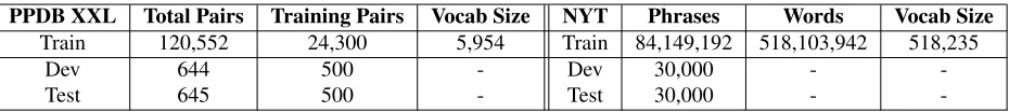
PPDB XXL Total Pairs Training Pairs Vocab Size NYT Phrases Words Vocab Size

Train 120,552 24,300 5,954 Train 84,149,192 518,103,942 518,235

Dev 644 500 - Dev 30,000 -

-Test 645 500 - Test 30,000 -

-Table 2: Statistics of NYT and PPDB data. “Training pairs” are pairs of bigram phrase and word used in experiments.

word2vecembeddings, the LM objective, and the TASK-SPEC objective; as well as use hierarchical softmax training (HS) for language modeling exper-iments. We use a window sizec=5, the default of word2vec. We remove types that occur less than 5 times (default setting of word2vec). The vo-cabulary is the same for all evaluations. For NCE training we sample 15 words as negative samples for each training instance according to their frequencies in raw texts. Following Mikolov et al. (2013b) ifw has frequencyu(w)we set the sampling probability ofwtop(w) _∝ u(w)3/4. For HS training we build a Hoffman tree based on word frequency.

Pre-trained Word Embeddings For methods that require pre-trained lexical embeddings (FCT with pre-training,SUM(Section 5), and theFCTandRNN models in Section 6) we always use embeddings2 trained with the skip-gram model of word2vec. The embeddings are trained with NCE estimation using the same settings described above.

5 Experiments: Language Modeling

We begin with experiments on FCT for language modeling tasks (Section 3.1). The resultant em-beddings can then be used for pre-training in task-specific settings (Section 6).

Data We use the 1994-97 subset from the New York Times (NYT) portion of Gigaword v5.0 (Parker et al., 2011). Sentences are tokenized us-ing OpenNLP.3_{We removed words with frequencies} less than 5, yielding a vocabulary of 518,235 word forms and 515,301,382 tokens for training word em-beddings.

This dataset is used for both training baseline word embeddings and evaluating our models trained with the LM objective. When evaluating the LM task we consider bigram NPs in isolation (see the

2_{We use “input embeddings” learned byword2vec.} 3_{https://opennlp.apache.org/}

“Phrases” column in Table 2). For FCT features that require syntactic information, we extract the NYT portion of Annotated Gigaword (Napoles et al., 2012), which uses the Stanford parser’s anno-tations. We use all bigram noun phrases (obtained from the annotated data) as the input phrases for Eq. (3). A subset from January 1998 of NYT data is withheld for evaluation.

Baselines We include two baselines. The first is to use each component word to predict the context of the phrase with the skip gram model (Mikolov et al., 2013a) and then average the scores to get the probability (denoted asword2vec). The sec-ond is to use SUM of the skip-gram embeddings to predict the scores. Training the FCT models with pre-trained word embeddings requires running the skip-gram model on NYT data for 2 iterations: one for word2vectraining and one for learning FCT. Therefore, we also run the word2vec model for two epochs to provide embeddings for the baselines.

5.1 Results

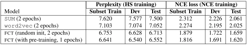
Perplexity (HS training) NCE loss (NCE training)

Model Subset Train Dev Test Subset Train Dev Test

SUM(2 epochs) 7.620 7.577 7.500 2.312 2.226 2.061

word2vec(2 epochs) 7.103 7.074 7.052 2.274 2.195 2.025

FCT(random init, 2 epochs) 6.753 6.628 6.713 1.879 1.722 1.659

FCT(with pre-training, 1 epochs) 6.641 6.540 6.552 1.816 1.691 1.620

Table 3: Language model perplexity and NCE loss on a subset of train, dev, and test NYT data.

kλ1k kλ2k kλ1k ≈ kλ2k kλ1k kλ2k

Model biological north-eastern dead medicinal new an

diversity part body products trial extension

FCT

sensitivity northeastern remains drugs proceeding signed natural sprawling grave uses cross-examination terminated abilities preserve skeleton chemicals defendant temporary

species area full

SUM

destruction portion unconscious marijuana new an racial result dying packaging judge renewal genetic integral flesh substances courtroom another

cultural chunk signing

Table 4: Differences in the nearest neighbors from the two phrase embedding models.

Table 3 shows results for the NYT training data (subset of the full training data containing 30,000 phrases with their contexts from July 1994), de-velopment and test data. Language models with FCT performed much better than the SUM and word2vec baselines, under both NCE and HS training. Note that FCT with pre-training makes a single pass over the whole NYT corpus and then a pass over only the bigram NPs, and the random initialization model makes a pass over the bigrams twice. This is less data compared to two passes over the full data (baselines), which indicates that FCT better captures the context distributions of phrases.

Qualitative Analysis Table 4 shows words and their most similar phrases (nearest neighbors) com-puted by FCT and SUM. We show three types of phrases: one where the two words in a phrase con-tribute equally to the phrase embedding, where the first word dominates the second in the phrase em-bedding, and vice versa. We measure the effect of each word by computing the total magnitude of the

λvector for each word in the phrase. For example,

for the phrase “an extension”, the embedding for the second word dominates the resulting phrase embed-ding (kλ1k kλ2k) as learned by FCT. The table

highlights the differences between the methods by showing the most relevant phrases not selected as most relevant by the other method. It is clear that words selected usingFCTare more semantically

re-lated than those of the baseline.

6 Experiments: Task-specific Training: Phrase Similarity

Data We consider several phrase similarity datasets for evaluating task-specific training. Table 5 summarizes these datasets and shows examples of inputs and outputs for each task.

PPDB The Paraphrase Database (PPDB)4 (Gan-itkevitch et al., 2013) contains tens of millions of automatically extracted paraphrase pairs, including words and phrases. We extract all paraphrases con-taining a bigram noun phrase and a noun word from PPDB. Since articles usually have little contribu-tions to the phrase meaning, we removed the easy cases of all pairs in which the phrase is composed of an article and a noun.Next, we removed duplicate pairs: if<A,B>occurred in PPDB, we removed re-lations of<B,A>. PPDB is organized into 6 parts, ranging from S (small) to XXXL. Division into these sets is based on an automatically derived accuracy metric. We extracted paraphrases from the XXL set. The most accurate (i.e. first) 1,000 pairs are used for evaluation and divided into a dev set (500 pairs) and test set (500 pairs); the remaining pairs were used for training. Our PPDB task is an extension of mea-suring PPDB semantic similarity between words (Yu

Data Set Input Output

(1)PPDB medicinal products drugs

(2)SemEval2013 <small spot, flect> True

<male kangaroo, point> False

(3)Turney2012 monosyllabic word monosyllable, hyalinization, fund, gittern, killer (4)PPDB (ngram) contribution of the european union eu contribution

Table 5: Examples of phrase similarity tasks. (1) PPDB is a ranking task, in which an input bigram and a output noun are given, and the goal is to rank the output word over other words in the vocabulary. (2)SemEval2013is a binary classification task: determine whether an input pair of a bigram and a word form a paraphrase (True) or not (False). (3)Turney2012is a multi-class classification task: determine the word most similar to the input phrase (in bold) from the five output candidates. For the 10-choice task, the goal is to select the most similar pair between the combination of one bigram phrase, i.e., the input phrase or the swapped input (“word monosyllabic” for this example), and the five output candidates. The correct answer in this case should still be the pair of original input phrase and the original correct output candidate (in bold). (4) PPDB (ngram) is similar to PPDB, but in which both inputs and outputs becomes noun phrases with arbitrary lengths.

and Dredze, 2014) to that between phrases. Data de-tails appear in Table 2.

Phrase Similarity Datasets We use a variety of human annotated datasets to evaluate phrase se-mantic similarity: the SemEval2013shared task (Korkontzelos et al., 2013), and the noun-modifier problem (Turney2012) in Turney (2012). Both tasks provide evaluation data and training data. Se-mEval2013 Task 5(a)is a classification task to de-termine if a word phrase pair are semantically simi-lar.Turney2012is a task to select the closest match-ing candidate word for a given phrase from candi-date words. The original task contained seven can-didates, two of which are component words of the input phrase (seven-choice task). Followup work has since removed the components words from the can-didates (five-choice task). Turney (2012) also pro-pose a 10-choice task based on this same dataset. In this task, the input bigram noun phrase will have its component words swapped. Then all the pairs of swapped phrase and a candidate word will be treated as a negative example. Therefore, each input phrase will correspond to 10 test examples where only one of them is the positive one.

Longer Phrases: PPDB (ngram-to-ngram) To show the generality of our approach we evaluate our method on phrases longer than bigrams. We extract arbitrary length noun phrase pairs from PPDB. We only include phrase pairs that differ by more than one word; otherwise the task would reduce to eval-uating unigram similarity. Similar to the

bigram-to-unigram task, we used the XXL set and removed du-plicate pairs. We used the most accurate pairs for development (2,821 pairs) and test (2,920 pairs); the remaining 148,838 pairs were used for training.

As before, we rely on negative sampling to effi-ciently compute the objective during training. For each source/target n-gram pair, we sample negative noun phrases as outputs. Both the target phrase and the negative phrases are transformed to their phrase embeddings with the current parameters. We then compute inner products between embedding of the source phrase and these output embeddings, and up-date the parameters according to the NCE objective. We use the same feature templates as in Table 1.

Notice that the XXL set contains several subsets (e.g., M, L ,XL) ranked by accuracy. In the experi-ments we also investigate their performance on dev data. Unless otherwise specified, the full set is se-lected (performs best on dev set) for training.

Baselines We compare to the common and ef-fective point-wise addition (SUM) method (Mitchell and Lapata, 2010).5 _{We additionally include}

Weighted SUM, which learns overall dimension specific weights from task-specific training, the equivalent ofFCTwithαjk=0andbij learned from

data. Furthermore, we compare to dataset specific

baselines: we re-implemented the recursive neural network model (RNN) (Socher et al., 2013a) and the Dual VSM algorithm in Turney (2012)6 _{so that} they can be trained on our dataset. We also include results for fine-tuning word embeddings in SUM and Weighted SUM with TASK-SPEC objectives, which demonstrate improvements over the corre-sponding methods without fine-tuning. As before, word embeddings are pre-trained withword2vec.

RNNs serve as another way to model the com-positionally of bigrams. We run an RNN on bi-grams and associated sub-trees, the same settingFCT uses, and are trained on our TASK-SPECobjectives with the technique described in Section 3.4. As in Socher et al. (2013a), we refine the matrix W in Eq. (5) according to the POS tags of the component words.7_{For example, for a bigram NP like new/ADJ} trial/NN, we use a matrixWADJ−N N to transform

the two word embeddings to the phrase embedding. In the experiments we have 60 different matrices in total for bigram NPs. The number is larger than that in Socher et al. (2013a) due to incorrect tags in au-tomatic parses.

Since theRNNmodel has time complexityO(n2), we compareRNNs with different sized embeddings. The first one uses embeddings with 50 dimensions, which has the same size as the embeddings used in Socher et al. (2013a), and has similar complexity to our model with 200 dimension embeddings. The second model uses the same 200 dimension embed-dings as our model but is significantly more compu-tationally expensive.

For all models, we normalize the embeddings so that the L-2 norm equals 1, which is important in measuring semantic similarity via inner product.

6.1 Results: Bigram Phrases

PPDB Our first task is to measure phrase simi-larity on PPDB. Training uses the TASK-SPEC ob-6_{We did not include results for a holistic model as in Turney} (2012), since most of the phrases (especially for those in PPDB) in our experiments are common phrases, making the vocabulary too large to train. One solution would be to only train holistic embeddings for phrases in the test data, but examination of a test set before training is not a realistic assumption.

7_{We do not compare the performance between using a single} matrix and several matrices since, as discussed in Socher et al. (2013a),Ws refined with POS tags work much better than using

a singleW. That also supports the argument in this paper, that it is important to determine the transformation with more features.

10^3 10^4 10^5

34 36 38 40 42 44 46 48 50 52 54

Vocabulary Sizes

MRR on Test Set(%)

SUM RNN50 RNN200 FCT

(a) MRR of models with fixed word embeddings

10^3 10^4 10^5

35 40 45 50 55 60 65 70

Vocabulary Sizes

MRR on Test Set(%)

SUM RNN50 RNN200 FCT FCT−pipeline FCT−joint

(b) MRR of models with fine-tuning

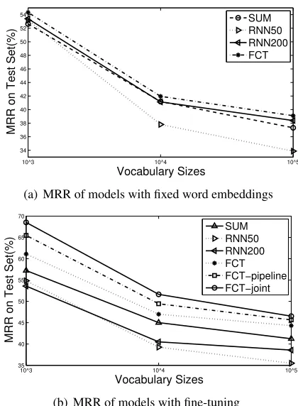
Figure 1: Performance on PPDB task (test set).

jective (Eq. (4) with NCE training) where data are phrase-word pairs< A,B >. The goal is to select Bfrom a set of candidates givenA, where pair sim-ilarity is measured using inner product. We use can-didate sets of size 1k/10k/100k from the most fre-quent N words in NYT and report mean reciprocal rank (MRR).

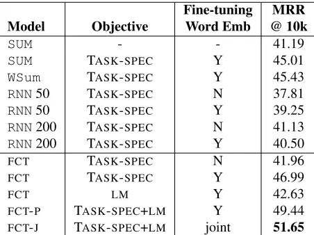
We report results with the baseline methods (SUM, Weighted SUM,RNN). For FCTwe report training with the TASK-SPEC objective, the joint-objective (FCT-J) and the pipeline approach (FCT-P). To en-sure that the TASK-SPECobjective has a stronger in-fluence inFCT-Joint, we weighted each training in-stance ofLMby 0.01, which is equivalent to setting the learning rate of theLMobjective equal toη/100 and that of the TASK-SPEC objective as η. Train-ing makes the same number of passes with the same learning rate as training with the TASK-SPEC objec-tive only. For each method we report results with and without fine-tuning the word embeddings on the labeled data. We runFCTon the PPDB training data for 5 epochs with learning rateη = 0.05, which are both selected from development set.

differ-Fine-tuning MRR

Model Objective Word Emb @ 10k

SUM - - 41.19

SUM TASK-SPEC Y 45.01

WSum TASK-SPEC Y 45.43

RNN50 TASK-SPEC N 37.81

RNN50 TASK-SPEC Y 39.25

RNN200 TASK-SPEC N 41.13

RNN200 TASK-SPEC Y 40.50

FCT TASK-SPEC N 41.96

FCT TASK-SPEC Y 46.99

FCT LM Y 42.63

FCT-P TASK-SPEC+LM Y 49.44

FCT-J TASK-SPEC+LM joint 51.65

Table 6: Performance on the PPDB task (test data).

ent candidate vocabulary sizes (1k, 10k and 100k), and Table 6 highlights the results on the vocabulary using the top 10k words. Overall, FCTwith TASK-SPEC training improves over all the baseline meth-ods in each setting. Fine-tuning word embeddings improves all methods except RNN (d=200). We note that theRNNperforms poorly, possibly because it uses a complex transformation from word em-bedding to phrase emem-beddings, making the learned transformation difficult to generalize well to new phrases and words when the task-specific labeled data is small. As a result, there is no guarantee of comparability between new pairs of phrases and word embeddings. The phrase embeddings may end up in a different part of the subspace from the word embeddings.

Comparing to SUM and Weighted SUM, FCT is capable of using features providing critical con-textual information, which is the source of FCT’s improvement. Additionally, since the RNNs also used POS tags and parsing information yet achieved lower scores than FCT, our results show that FCT more effectively uses these features. To better show this advantage, we trainFCTmodels with only POS tag features, which achieve 46.37/41.20 on MRR@10k with/without fine-tuning word embed-dings, still better thanRNNs. See Section 6.3 for a full ablation study of features in Table 1.

Semi-supervised Results: Table 6 also high-lighted the improvement from semi-supervised learning. First, the fully unsupervised method (LM)

improves over SUM, showing that improvements in language modeling carry over to semantic similar-ity tasks. This correlation between the LM ob-jective and the target task ensures the success of supervised training. As a result, both semi-supervised methods,FCT-JandFCT-Pimproves over the supervised methods; and FCT-J achieves the best results of all methods, including FCT-P. This demonstrates the effectiveness of including large amounts of unlabeled data while learning with a TASK-SPEC objective. We believe that by adding theLMobjective, we can propagate the semantic in-formation of embeddings to the words that do not appear in the labeled data (see the differences be-tween vocabulary sizes in Table 2).

The improvement of FCT-J over FCT-P also in-dicates that the joint training strategy can be more effective than the traditional pipeline-based pre-training. As discussed in Section 3.3, the pipeline method, although commonly used in deep learning literatures, does not suit NLP applications well be-cause of the sparsity in word embeddings. There-fore, our results suggest an alternative solution to a wide range of NLP problems where labeled data has low coverage of the vocabulary. For future work, we will further investigate the idea of joint training on more tasks and compare with the pipeline method.

Results on SemEval2013 and Turney2012 We evaluate the same methods onSemEval2013and the Turney2012 5- and 10-choice tasks, which both provide training and test splits. The same base-lines in the PPDB experiments, as well as the Dual Space method of Turney (2012) and the recursive auto-encoder (RAE) from Socher et al. (2011) are used for comparison. Since the tasks did not provide any development data, we used cross-validation (5 folds) for tuning the parameters, and finally set the training epochs to be 20 and η = 0.01. For joint training, the weight of theLMobjective is weighted by 0.005 (i.e. with a learning rate equal to0.005η) since the training sets for these two tasks are much smaller. For convenience, we also include results for Dual Space as reported in Turney (2012), though they are not comparable here since Turney (2012) used a much larger training set.

dimen-Fine-tuning SemEval2013 Turney2012

Model Objective Word Emb Test Acc (5) Acc (10) MRR @ 10k

SUM - - 65.46 39.58 19.79 12.00

SUM TASK-SPEC Y 67.93 48.15 24.07 14.32

Weighted Sum TASK-SPEC Y 69.51 52.55 26.16 14.74

RNN(d=50) TASK-SPEC N 67.20 39.64 25.35 1.39

RNN(d=50) TASK-SPEC Y 70.36 41.96 27.20 1.46

RNN(d=200) TASK-SPEC N 71.50 40.95 27.20 3.89

RNN(d=200) TASK-SPEC Y 72.22 42.84 29.98 4.03

Dual Space1 _{- - 52.47 27.55 16.36 2.22}

Dual Space2 _{- - - 58.3 41.5}

-RAE auto-encoder - 51.75 22.99 14.81 0.16

FCT TASK-SPEC N 68.84 41.90 33.80 8.50

FCT TASK-SPEC Y 70.36 52.31 38.66 13.19

FCT LM - 67.22 42.59 27.55 14.07

FCT-P TASK-SPEC+LM Y 70.64 53.09 39.12 14.17

FCT-J TASK-SPEC+LM joint 70.65 53.31 39.12 14.25

Table 7: Performance onSemEval2013andTurney2012semantic similarity tasks. Dual Space1_{: Our} reimple-mentation of the method in (Turney, 2012). Dual Space2_{: The result reported in Turney (2012). RAEis the recursive} auto-encoder in (Socher et al., 2011), which is trained with the reconstruction-based objective of auto-encoder.

sional embeddings onSemEval2013, though at a dimensionality with similar computational complex-ity toFCT(d= 50),FCTimproves. Additionally, on the 10-choice task ofTurney2012, both the FCT and the RNN models, either with or without fine-tuning word embeddings, significantly outperform SUM, showing that both models capture the word or-der information. Fine tuning gives smaller gains on RNNs likely because the limited number of training examples is insufficient for the complexRNNmodel. TheLMobjective leads to improvements on all three tasks, whileRAEdoes not perform significantly bet-ter than random guessing. These results are perhaps attributable to the lack of assumptions in the objec-tive about the relations between word embeddings and phrase embeddings, making the learned phrase embeddings not comparable to word embeddings.

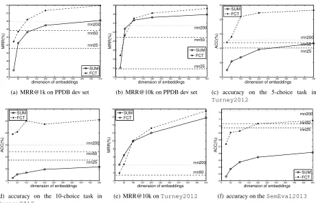
6.2 Dimensionality and Complexity

A benefit of FCT is that it is computationally effi-cient, allowing it to easily scale to embeddings of 200 dimensions. By contrast, RNN models typi-cally use smaller sized embeddings (d= 25proved best in Socher et al., 2013a) and cannot scale up to large datasets when larger dimensionality embed-dings are used. For example, when training on the PPDB data, the FCT with d = 200processes 2.33 instances per ms, while theRNN with the same

di-mensionality processes 0.31 instance/ms. Training anRNNwithd= 50is of comparable speed toFCT with d = 200. Figure 2 (a-b) shows the MRR on PPDB for 1k and 10k candidate sets for both the SUMbaseline andFCTwith a TASK-SPECobjective and full features, as compared toRNNs with differ-ent sized embeddings. BothFCTandRNN use fine-tuned embeddings. With a small number of embed-ding dimensions,RNNs achieve better results. How-ever, FCT can scale to much higher dimensionality embeddings, which easily surpasses the results of RNNs. This is especially important when learning a large number of embeddings: the 25-dimensional space may not be sufficient to capture the semantic diversity, as evidenced by the poor performance of RNNs with lower dimensionality.

0 50 100 150 200 250 300 350 400 450 500 34 36 38 40 42 44 46 48 50 52 rnn25 rnn50 rnn200

dimension of embeddings

MRR(%)

SUM FCT

(a) MRR@1k on PPDB dev set

0 50 100 150 200 250 300 350 400 450 500 22 24 26 28 30 32 34 36 38

dimension of embeddings

MRR(%) rnn25 rnn50 rnn200 SUM FCT

(b) MRR@10k on PPDB dev set

0 50 100 150 200 250 300 350 400 450 500 30 35 40 45 50 55 rnn25 rnn50 rnn200

dimension of embeddings

ACC(%)

SUM FCT

(c) accuracy on the 5-choice task in

Turney2012

0 50 100 150 200 250 300 350 400 450 500 15 20 25 30 35 40 45 rnn25 rnn50 rnn200

dimension of embeddings

ACC(%)

SUM FCT

(d) accuracy on the 10-choice task in

Turney2012

0 50 100 150 200 250 300 350 400 450 500 0 2 4 6 8 10 12 14 16 18

dimension of embeddings

MRR(%)

rnn50 rnn200 SUM

FCT

(e) MRR@10k onTurney2012

0 50 100 150 200 250 300 350 400 450 500 62 63 64 65 66 67 68 69 70 71 72 rnn25 rnn50 rnn200

dimension of embeddings

ACC(%)

SUM FCT

(f) accuracy on theSemEval2013

Figure 2: Effects of embedding dimension on the semantic similarity tasks. The notations “RNN< d >” in the figures stand for theRNNmodels trained withd-dimensional embeddings.

which is critical to solving the 10-choice task, with-out relying on too much semantic information from word embeddings themselves. Figure 2(e) shows that when the dimensionality of embeddings is lower than 100, bothFCTandRNNdo worse than the base-line. This is likely because in the case of low dimen-sionality, updating embeddings is likely to change the whole structure of embeddings of training words, making both the fine-tuned word embeddings and the learned phrase embeddings incomparable to the other words. The performance of RNN with 25-dimension embeddings is too low so it is omitted.

6.3 Experiments on Longer Phrases

So far our experiments have focused on bigram phrases. We now show thatFCTimproves for longer n-gram phrases (Table 8). Without fine-tuning,FCT performs significantly better than the other models, showing that the model can better capture the con-text and annotation information related to phrase se-mantics with the help of rich features. With different amounts of training data, we found that WSum and FCTboth perform better when trained on the

PPDB-Train Fine-tuning MRR

Model Set Word Emb @10k @ 100k

SUM - N 46.53 16.62

WSum L N 51.10 18.92

FCT L N 68.91 29.04

SUM XXL Y 74.30 29.14

WSum XXL Y 75.37 31.13

FCT XXL Y 79.68 36.00

Table 8: Results onPPDB ngram-to-ngramtask.

L set, a more accurate subset of XXL with 24,279 phrase pairs. This can be viewed as a low resource setting, where there is limited data for fine-tuning word embeddings.

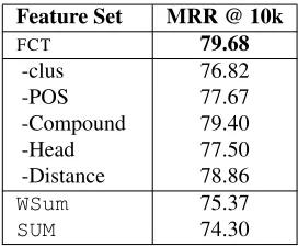
Feature Set MRR @ 10k

FCT 79.68

-clus 76.82

-POS 77.67

-Compound 79.40

-Head 77.50

-Distance 78.86

WSum 75.37

SUM 74.30

Table 9: Ablation study on dev set of the PPDB ngram-to-ngramtask (MRR @ 10k).

by the quality of single word semantics. Therefore, we expect larger gains fromFCTon tasks where sin-gle word embeddings are less important, such as re-lation extraction (long distance dependencies) and question understanding (intentions are largely de-pendent on interrogatives).

Finally, we demonstrate the efficacy of different features inFCT(Table 1) with an ablation study (Ta-ble 9). Word cluster features contribute most, be-cause the point-wise product between word embed-ding and its context word cluster representation is actually an approximation of the word-word inter-action, which is believed important for phrase com-positions. Head features, though few, also make a big difference, reflecting the importance of syntactic information. Compound features do not have much of an impact, possibly because the simpler features capture enough information.

7 Related Work

Compositional semantic models aim to build distri-butional representations of a phrase from its compo-nent word representations. A traditional approach for composition is to form a point-wise combina-tion of single word representacombina-tions with composi-tional operators either pre-defined (e.g. element-wise sum/multiplication) or learned from data (Le and Mikolov, 2014). However, these approaches ignore the inner structure of phrases, e.g. the or-der of words in a phrase and its syntactic tree, and the point-wise operations are usually less expressive. One solution is to apply a matrix transformation (possibly followed by a non-linear transformation) to the concatenation of component word represen-tations (Zanzotto et al., 2010). For longer phrases,

matrix multiplication can be applied recursively ac-cording to the associated syntactic trees (Socher et al., 2010). However, because the input of the model is the concatenation of word representations, ma-trix transformations cannot capture interactions be-tween a word and its contexts, or bebe-tween compo-nent words.

There are three ways to restore these interac-tions: The first is to use word-specific/tensor trans-formations to force the interactions between com-ponent words in a phrase. In these methods, word-specific transformations, which are usually matri-ces, are learned for a subset of words according to their syntactic properties (e.g. POS tags) (Baroni and Zamparelli, 2010; Socher et al., 2012; Grefen-stette et al., 2013; Erk, 2013). Composition between a word in this subset and another word becomes the multiplication between the matrix associated with one word and the embedding of the other, produc-ing a new embeddproduc-ing for the phrase. Usproduc-ing one tensor (not word-specific) to compose two embed-ding vectors (has not been tested on phrase similar-ity tasks) (Bordes et al., 2014; Socher et al., 2013b) is a special case of this approach, where a “word-specific transformation matrix” is derived by multi-plying the tensor and the word embedding. Addi-tionally, word-specific matrices can only capture the interaction between a word and one of its context words; others have considered extensions to multi-ple words (Grefenstette et al., 2013; Dinu and Ba-roni, 2014). The primary drawback of these ap-proaches is the high computational complexity, lim-iting their usefulness for semantics (Section 6.2.)

em-beddings of component words still cannot interact, they can interact with other information (i.e. fea-tures) of their context words, and even the global features. Recent research has created novel features based on combining word embeddings and contex-tual information (Nguyen and Grishman, 2014; Roth and Woodsend, 2014; Kiros et al., 2014; Yu et al., 2014; Yu et al., 2015). Yu et al. (2015) further pro-posed converting the contextual features into a hid-den layer called feature embeddings, which is sim-ilar to the αmatrix in this paper. Examples of ap-plications to phrase semantics include Socher et al. (2013a) and Hermann and Blunsom (2013), who en-hanced RNNs by refining the transformation matri-ces with phrase types and CCG super tags. How-ever, these models are only able to use limited infor-mation (usually one property for each compositional transformation), whereasFCTexploits multiple fea-tures.

Finally, our work is related to recent work on low-rank tensor approximations. When we use the phrase embedding ep in Eq. (1) to predict a label

y, the score of y given phrase p will bes(y, p) = UT

y ep = PNi UyT(λi ewi) in log-linear models,

where Uy is the parameter vector for y. This is

equivalent to using a parameter tensorT to evaluate the score withs0(y, p) =PN_i T_×1y×2f(wi, p)×

ewi, while forcing the tensor to have a low-rank form

asT ≈U⊗α⊗ew. Here×kindicates tensor

mul-tiplication of thekth view, and ⊗indicates matrix outer product (Kolda and Bader, 2009). From this point of view, our work is closely related to the dis-criminative training methods for low-rank tensors in NLP (Cao and Khudanpur, 2014; Lei et al., 2014), while it can handle more complex ngram-to-ngram tasks, where the labelyalso has its embedding com-posed from basic word embeddings. Therefore our model can capture the above work as special cases. Moreover, we have a different method of decompos-ing the inputs, which results in views of lexical parts and non-lexical features. As we show in this paper, this input decomposition allows us to benefit from pre-trained word embeddings and feature weights.

8 Conclusion

We have presentedFCT, a new composition model for deriving phrase embeddings from word

embed-dings. Compared to existing phrase composition models,FCTis very efficient and can utilize high di-mensional word embeddings, which are crucial for semantic similarity tasks. We have demonstrated howFCTcan be utilized in a language modeling set-ting, as well as tuned with task-specific data. Fine-tuning embeddings on task-specific data can further improve FCT, but combining both LM and TASK-SPEC objectives yields the best results. We have demonstrated improvements on both language mod-eling and several semantic similarity tasks. Our im-plementation and datasets are publicly available.8

While our results demonstrate improvements for longer phrases, we still only focus on flat phrase structures. In future work we plan toFCT with the idea of recursively building representations. This would allow the utilization of hierarchical structure while restricting compositions to a small number of components.

Acknowledgments

We thank Matthew R. Gormley for his input and anonymous reviewers for their comments. Mo Yu is supported by the China Scholarship Council and by NSFC 61173073.

References

Marco Baroni and Roberto Zamparelli. 2010. Nouns are vectors, adjectives are matrices: Representing adjective-noun constructions in semantic space. In Empirical Methods in Natural Language Processing

(EMNLP), pages 1183–1193.

Yoshua Bengio, R´ejean Ducharme, Pascal Vincent, and Christian Janvin. 2003. A neural probabilistic lan-guage model. The Journal of Machine Learning

Re-search (JMLR), 3:1137–1155.

Antoine Bordes, Xavier Glorot, Jason Weston, and Yoshua Bengio. 2014. A semantic matching energy function for learning with multi-relational data.

Ma-chine Learning, 94(2):233–259.

Yuan Cao and Sanjeev Khudanpur. 2014. Online learn-ing in tensor space. InAssociation for Computational

Linguistics (ACL), pages 666–675.

Jackie Chi Kit Cheung and Gerald Penn. 2013. Prob-abilistic domain modelling with contextualized distri-butional semantic vectors. InAssociation for

Compu-tational Linguistics (ACL), pages 392–401.

Ronan Collobert and Jason Weston. 2008. A unified ar-chitecture for natural language processing: Deep neu-ral networks with multitask learning. InInternational

Conference on Machine Learning (ICML), pages 160–

167.

Ronan Collobert. 2011. Deep learning for efficient dis-criminative parsing. In International Conference on

Artificial Intelligence and Statistics (AISTATS), pages

224–232.

Georgiana Dinu and Marco Baroni. 2014. How to make words with vectors: Phrase generation in distributional semantics. InAssociation for Computational

Linguis-tics (ACL), pages 624–633.

Georgiana Dinu and Mirella Lapata. 2010. Measuring distributional similarity in context. InEmpirical

Meth-ods in Natural Language Processing (EMNLP), pages

1162–1172.

Katrin Erk and Sebastian Pad´o. 2008. A structured vector space model for word meaning in context. In Empirical Methods in Natural Language Processing

(EMNLP), pages 897–906.

Katrin Erk. 2013. Towards a semantics for distributional representations. InInternational Conference on

Com-putational Semantics (IWCS 2013), pages 95–106.

Juri Ganitkevitch, Benjamin Van Durme, and Chris Callison-Burch. 2013. Ppdb: The paraphrase database. In North American Chapter of the

Associ-ation for ComputAssoci-ational Linguistics (NAACL), pages

758–764.

Edward Grefenstette, Georgiana Dinu, Yao-Zhong Zhang, Mehrnoosh Sadrzadeh, and Marco Baroni. 2013. Multi-step regression learning for composi-tional distribucomposi-tional semantics.arXiv:1301.6939. Karl Moritz Hermann and Phil Blunsom. 2013. The role

of syntax in vector space models of compositional se-mantics. InAssociation for Computational Linguistics

(ACL), pages 894–904.

Karl Moritz Hermann, Dipanjan Das, Jason Weston, and Kuzman Ganchev. 2014. Semantic frame identifi-cation with distributed word representations. In

As-sociation for Computational Linguistics (ACL), pages

1448–1458.

Eric H Huang, Richard Socher, Christopher D Manning, and Andrew Y Ng. 2012. Improving word representa-tions via global context and multiple word prototypes.

In Association for Computational Linguistics (ACL),

pages 873–882.

Ryan Kiros, Richard Zemel, and Ruslan R Salakhutdinov. 2014. A multiplicative model for learning distributed text-based attribute representations. In Advances in

Neural Information Processing Systems (NIPS), pages

2348–2356.

Tamara G Kolda and Brett W Bader. 2009. Ten-sor decompositions and applications. SIAM review, 51(3):455–500.

Ioannis Korkontzelos, Torsten Zesch, Fabio Massimo Zanzotto, and Chris Biemann. 2013. Semeval-2013 task 5: Evaluating phrasal semantics. InJoint Con-ference on Lexical and Computational Semantics (* SEM), pages 39–47.

Quoc V Le and Tomas Mikolov. 2014. Distributed repre-sentations of sentences and documents. arXiv preprint

arXiv:1405.4053.

Tao Lei, Yu Xin, Yuan Zhang, Regina Barzilay, and Tommi Jaakkola. 2014. Low-rank tensors for scoring dependency structures. In Association for

Computa-tional Linguistics (ACL), pages 1381–1391.

Tomas Mikolov, Kai Chen, Greg Corrado, and Jeffrey Dean. 2013a. Efficient estimation of word representa-tions in vector space.arXiv preprint arXiv:1301.3781. Tomas Mikolov, Ilya Sutskever, Kai Chen, Greg Corrado, and Jeffrey Dean. 2013b. Distributed representations of words and phrases and their compositionality. arXiv

preprint arXiv:1310.4546.

Jeff Mitchell and Mirella Lapata. 2008. Vector-based models of semantic composition. In Association for

Computational Linguistics (ACL), pages 236–244.

Jeff Mitchell and Mirella Lapata. 2010. Composition in distributional models of semantics. Cognitive science, 34(8):1388–1429.

Courtney Napoles, Matthew Gormley, and Benjamin Van Durme. 2012. Annotated gigaword. InACL Joint Workshop on Automatic Knowledge Base Construction

and Web-scale Knowledge Extraction, pages 95–100.

Thien Huu Nguyen and Ralph Grishman. 2014. Employ-ing word representations and regularization for domain adaptation of relation extraction. In Association for

Computational Linguistics (ACL), pages 68–74.

Robert Parker, David Graff, Junbo Kong, Ke Chen, and Kazuaki Maeda. 2011. English gigaword fifth edition, june. Linguistic Data Consortium, LDC2011T07. Michael Roth and Kristian Woodsend. 2014.

Compo-sition of word representations improves semantic role labelling. InEmpirical Methods in Natural Language

Processing (EMNLP), pages 407–413.

Richard Socher, Christopher D Manning, and Andrew Y Ng. 2010. Learning continuous phrase representa-tions and syntactic parsing with recursive neural net-works. InNIPS Workshop on Deep Learning and

Un-supervised Feature Learning, pages 1–9.

Richard Socher, Jeffrey Pennington, Eric H Huang, An-drew Y Ng, and Christopher D Manning. 2011. Semi-supervised recursive autoencoders for predicting sen-timent distributions. InEmpirical Methods in Natural

Richard Socher, Brody Huval, Christopher D Manning, and Andrew Y Ng. 2012. Semantic compositionality through recursive matrix-vector spaces. InEmpirical

Methods in Natural Language Processing (EMNLP),

pages 1201–1211.

Richard Socher, John Bauer, Christopher D. Manning, and Ng Andrew Y. 2013a. Parsing with compositional vector grammars. In Association for Computational

Linguistics (ACL), pages 455–465.

Richard Socher, Alex Perelygin, Jean Wu, Jason Chuang, Christopher D. Manning, Andrew Ng, and Christo-pher Potts. 2013b. Recursive deep models for se-mantic compositionality over a sentiment treebank. In Empirical Methods in Natural Language Processing

(EMNLP), pages 1631–1642.

Stefan Thater, Hagen F¨urstenau, and Manfred Pinkal. 2011. Word meaning in context: A simple and ef-fective vector model. In International Joint

Con-ference on Natural Language Processing (IJCNLP),

pages 1134–1143.

Joseph Turian, Lev Ratinov, and Yoshua Bengio. 2010. Word representations: a simple and general method for semi-supervised learning. InAssociation for

Compu-tational Linguistics (ACL), pages 384–394.

Peter D Turney. 2012. Domain and function: A dual-space model of semantic relations and compo-sitions. Journal of Artificial Intelligence Research

(JAIR), 44:533–585.

Mo Yu and Mark Dredze. 2014. Improving lexical em-beddings with semantic knowledge. InAssociation for

Computational Linguistics (ACL), pages 545–550.

Mo Yu, Matthew Gormley, and Mark Dredze. 2014. Factor-based compositional embedding models. In

NIPS Workshop on Learning Semantics.

Mo Yu, Matthew R. Gormley, and Mark Dredze. 2015. Combining word embeddings and feature embeddings for fine-grained relation extraction. InNorth American Chapter of the Association for Computational

Linguis-tics (NAACL).

Fabio Massimo Zanzotto, Ioannis Korkontzelos, Francesca Fallucchi, and Suresh Manandhar. 2010. Estimating linear models for compositional distri-butional semantics. In International Conference

on Computational Linguistics (COLING), pages