Training Multilayered Perceptrons for Pattern
Recognition: A Comparative Study of Five
Training Algorithms
N.V.N. Indra Kiran1, M.Pramiladevi Devi 2 and G.Vijaya Lakshmi 3
Abstract -Control charts pattern recognition is one of the most important tools in statistical process control to identify process problems. Unnatural patterns exhibited by such charts can be associated with certain assignable causes affecting the process. In this paper a study is carried out on training algorithms for CCPs recognition and the best one is identified for type I and type II errors for generalization without early stopping and with early stopping.
Index
terms-Control chart pattern recognition, neural network, backpropagation, generalization, early stopping
I. INTRODUCTION
There are seven basic CCPs, e.g. normal (NOR), systematic (SYS), cyclic (CYC), increasing trend (IT), decreasing trend (DT), upward shift(US) and downward shift (DS) [6]. All other patterns are either special forms of basic CCPs or mixed forms of two or more basic CCPs. Only the NOR pattern is indicative of a process continuing to operate under controlled condition. All other CCPs are unnatural and associated with impending problems requiring pre-emptive actions. ANN learns to recognize patterns directly through a typical sample patterns during a training phase. Neural nets may provide required abilities to replace the human operator. Neural network also have the ability to identify an arbitrary Pattern not previously encountered. Back propagation network (BPN) has been widely used to recognize different abnormal patterns of a control chart [2], [8], [9], [10].BPN is a supervised-learning network and its output value is Continuous, usually between zero and one. It is usually used for detecting, forecasting and classification tasks, and is one of the most commonly used networks [3].
Manuscript received June 19, 2010; revised November 03, 2010 1. N.V.N.Indra Kiran is with the ANITS engineering
college,visakhapatnam INDIA e-mail: [email protected]. 2. M.Pramila devi is with the Andhra university engineering college,visakhapatnam INDIA e-mail: [email protected] 3. G.Vijaya Lakshmi is with the Kaushik engineering
college,visakhapatnam INDIA e-mail: [email protected]
II. PATTERN RECOGNIZER DESIGN
A. Sample patterns
Sample patterns should be collected from a real manufacturing process. Since, a large number of patterns are required for developing and validating a CCP recognizer, and as those are not economically available, simulated data are often used. Since a large window size can decrease the recognition efficiency by increasing the time required to detect the patterns, an observation window with 32 data points is considered here. The values of different parameters for the unnatural patterns are randomly varied in a uniform manner. A set of 3500 (500x7) sample patterns are generated from 500 series of standard normal variates. The equations used for simulating the seven CCPs are given in Appendix A.
B. Training algorithms
It is very difficult to know which training algorithm will be the fastest for a given problem. It depends on many factors, including the complexity of the problem, the number of data points in the training set, the number of weights and biases in the network, the error goal, and this section compares the various training algorithms.
. In backpropagation, the gradient is determined by performing computations backwards through the network [3]. There are many variations of backpropagation, some of them provide faster convergence while others give smaller memory requirement. In this study five training algorithms are evaluated they are gradient descent algorithm (traindx) and resilient backpropagation (trainrp), Conjugate Gradient Algorithms (trainscg), Quasi-Newton Algorithms (trainbfg) and Levenberg-Marquardt (trainlm) [4].
able to obtain lower mean square errors than any of the other algorithms tested. However, as the number of weights in the network increases, the advantage of trainlm decreases. In addition, trainlm performance is relatively poor on pattern recognition problems. The storage requirements of trainlm are larger than the other algorithms tested. The trainrp function is the fastest algorithm on pattern recognition problems. Its performance also degrades as the error goal is reduced. The memory requirements for this algorithm are relatively small in comparison to the other algorithms considered.
Based on the experiments are coded in MATLAB® using its ANN toolbox [4].The traindx , trainrp, trainlm, trainscg, trainbfg is adopted here for training of the network, since they provide reasonably good performance and more consistent results for the problem are under study.
C. Neural network configuration
The recognizer was developed based on multilayer perceptions (MLPs) architecture; Its structure comprises an input layer, one or more hidden layer(s) and an output layer. Figure 1 shows an MLP neural network structure comprising these layers and their respective weight connections. Before this recognizer can be put into application, it needs to be trained and tested. In the supervised training approach, sets of training data comprising input and target vectors are presented to the MLP. The learning process takes place through adjustment of weight connections between the input and hidden layers and between the hidden and output layers. These weight connections are adjusted according to the specified performance and learning functions. The input node size was equal to the size of the observation window, i.e. 32. The number of output nodes in this study was set corresponding to the number of pattern classes, i.e. seven. The labels, shown in table 1, are the targeted values for the recognizers’ output nodes. The maximum value in each row (0.9) identifies the corresponding node expected to secure the highest output for a pattern to be considered correctly classified.
Figure1. MLP neural network architecture
The general rule is that the network size should be as small as possible to allow efficient computation. The number of nodes in the hidden layer is selected based on the results of many experiments conducted by varying the number of nodes from 11 to 20. All those experiments are coded in MATLAB® using its ANN toolbox [4] for the two selected algorithms traindx, trainrp. The transfer functions used are hyperbolic tangent (tansig) for the hidden layer and sigmoid (logsig) for the output layer. The hyperbolic tangent function transforms the layer inputs to output range from −1 to +1 and the sigmoid function transforms the layer inputs to output range from 0 to 1 [12].
Table1: Targeted recognizer outputs
Pattern
class
Recognizer outputs node
1 2 3 4 5 6 7
NOR 0.9 0.1 0.1 0.1 0.1 0.1 0.1
SYS 0.1 0.9 0.1 0.1 0.1 0.1 0.1
CYC 0.1 0.1 0.9 0.1 0.1 0.1 0.1
IT 0.1 0.1 0.1 0.9 0.1 0.1 0.1
DT 0.1 0.1 0.1 0.1 0.9 0.1 0.1
US 0.1 0.1 0.1 0.1 0.1 0.9 0.1
DS 0.1 0.1 0.1 0.1 0.1 0.1 0.9
Table2: nnhl for training algorithms
nnhl dx rp lm scg bfg
11 0.9090 0.8545 0.8640 0.8218 0.6922
12 0.9134 0.9169 0.8630 0.8995 0.7279
13 0.8765 0.8500 0.5664 0.8761 0.7636
14 0.9080 0.8946 0.5925 0.8869 0.7848
15 0.9217 0.8739 0.6969 0.8509 0.7827
16 0.9348 0.900 0.7699 0.9218 0.8314
17 0.9210 0.9329 0.6962 0.9028 0.8389
18 0.9114 0.8784 0.5810 0.8689 0.7315
19 0.8780 0.9181 0.8819 0.9103 0.7881
20 0.8825 0.9198 0.7611 0.9000 0.8151
NNHL: number of neurons in hidden layer
Input layer
Hidden layer
Output layer
Input values
Coefficient of correlation performance of the neural network for the algorithms is the maximum when the number of nodes in the hidden layer is shown bolded in table 2.The selected ANN architecture is given below.
Network details: traindx: Architecture: 32-16-7 network,
with tansig TF and logsig TF in hidden and output layer respectively. Training: traindx algorithm
Network details: trainrp: Architecture: 32-17-7 network,
with tansig TF and logsig TF in hidden and output layer respectively. Training: trainrp algorithm
Network details: trainlm: Architecture: 32-19-7 network,
with tansig TF and logsig TF in hidden and output layer respectively. Training: trainlm algorithm
Network details: trainscg: Architecture: 32-16-7 network,
with tansig TF and logsig TF in hidden and output layer respectively. Training: trainscg algorithm
Network details: trainbfg: Architecture: 32-17-7 network,
with tansig TF and logsig TF in hidden and output layer respectively. Training: trainbfg algorithm
D Generalization
Improving Generalization
One of the problems that occur during neural network training is called over fitting. The error on the training set is driven to a very small value, but when new data is presented to the network the error is large. The network has memorized the training examples, but it has not learned to generalize to new situations for improving generalization early stopping is used and it is implemented in Neural Network Toolbox software[4].
Early Stopping
In this technique the available data is divided into three subsets. The first subset is the training set, which is used for computing the gradient and updating the network weights and biases. The second subset is the validation set. The error on the validation set is monitored during the training process. The validation error normally decreases during the initial phase of training, as does the training set error. However, when the network begins to over fit the data, the error on the validation set typically begins to rise. When the validation error increases for a specified number of iterations (net.trainParam.max_fail=5), the training is stopped, and the weights and biases at the minimum of the validation error are returned.
III. EXPERIMENTAL PROCEDURE
ANN recognizers was developed using raw data as the input vector. This section discusses the procedures for the training and recall (recognition) phases of the recognizers. The recognition task was limited to the seven previously
mentioned common SPC chart patterns. All the procedures were coded in MATLAB using its ANN toolbox [4].
A Training phase
The overall procedure began with the generation and presentation of process data to the observation window. All patterns were fully developed when they appeared within the recognition window. For raw data as the input vector, the pre-processing stage involved basic transformation into standardized Normal (0, 1) values[5]. Before the sample data were presented to the ANN for the learning process, it was divided into training (60%), validation (20%) and preliminary testing (20%) sets (Demuth and Beale 1998). These sample sets were then randomized to avoid possible bias in the presentation order of the sample patterns to the ANN. The training procedure was conducted iteratively covering ANN learning, validation of in-training ANN and preliminary testing. During learning, a training data set (2100 patterns) was used for updating the network weights and biases. The ANN was then subjected to in-training validation using the validation data set (700patterns) for early stopping to avoid over fitting. The error on the validation set will typically begin to rise when the network begins to over fit the data. The training process was stopped when the validation error increases for a specified number of iterations. In this study, the maximum number of validation failures was set to five iterations. The ANN was then subjected to preliminary performance tests using the testing data set (700 patterns).The testing set errors were not used for updating the network weights and biases. The training was stopped whenever one of the following stopping criteria was satisfied. The performance error goal was achieved, the maximum allowable number of training epochs was met or the maximum number of validation failures was exceeded (validation test).Once the training stopped, the trained recognizer was evaluated for acceptance. The recognizer would be retrained using a totally new data set if its performance remained poor. This procedure was intended to minimize the effect of poor training sets. Each type of recognizer was replicated by exposing them to 3 different training cycles, giving rise to 3 different trained recognizers for early stopping and 3 different trained recognizers without early stopping. All 6 recognizers for training algorithms have the same architecture and differ only in the training data sets used. Discussion on the training and recall performance provided in table 3 are given in section IV.
B. Recall or recognition phase
IV. RESULTS AND DISCUSSION
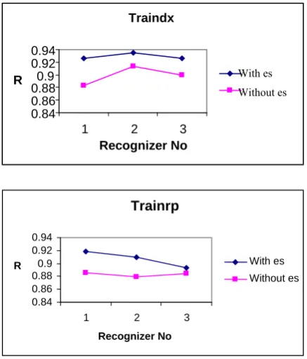
[image:4.595.307.549.67.399.2]This section presents results and comparisons of the performance between the recognizers trained and tested using five algorithms for generalization without early stopping and with early stopping. The recognition accuracy, coefficient of correlation (R) between actual targets and predicted targets and mean square error (mse) are higher compared to generalization obtained with early stopping than without early stopping for traindx algorithm.
Table 3 show the training and recall performance of the 3 raw data-based Recognizers for Traindx algorithm. Traindx provides better results in two categories. The overall recognition accuracy for five algorithms is shown in the table 4 and the graphs in figure 4.The type I error performance for both types of training algorithms does not seem to be very good. This is possibly due to the unpredictable structure of random data streams that make them relatively more difficult to be recognized compared with unstable patterns. On the other hand, unstable data streams have a tendency to correlate among the successive data. As such, the structures of their patterns are more predictable and this may have contributed towards easier recognition of unstable patterns. Type I error means wrong recognition that takes normal pattern as abnormal one and Type II error wrong recognition that takes abnormal pattern as normal one.
[image:4.595.48.267.448.704.2]
Figure 4. Comparisons of algorithms
Table 3. Computational results
Traindx with early stopping
Training Testing
R epoch Type I Type II Type I Type II
R1 0.926 156 91.11 99.18 90.4 98.76
R2 0.935 174 87.77 99.18 89.0 99.22
R3 0.926 170 91.11 99.34 87.0 99.00
Mean 0.929 166.6 89.99 99.23 88.8 98.99
Range 0.009 18 3.34 0.16 3.4 0.46
Traindx without early stopping
Training Testing
R epoch Type I Type II Type I Type II
R1 0.883 300 85.55 99.0 88.62 98.1
R2 0.912 300 87.77 99.34 88.40 98.69
R3 0.899 300 90.00 98.68 85.60 98.66
Mean 0.898 300 87.77 99.00 87.54 98.48
Range 0.029 0 4.45 0.66 3.02 0.68
Table4. Comparison of algorithms
Sl no
Recognition accuracy
withes Without es
1 traindx 94.25 92.22
2 trainrp 93.20 92.10
3 trainlm 85.95 88.20
4 trainscg 92.94 93.32
5 trainbfg 91.56 91.655
es: early stopping
V. CONCLUSIONS AND FUTURE WORK
The objective of this study was to evaluate the relative performance of training algorithms with the optimum structure for CCP recognizer. The MLP neural network was used as a generic recognizer to classify seven different types of SPC chart patterns. In this study five training algorithms are studied for generalization with early stopping and without early stopping and traindx is identified to be the best algorithm for this particular problem. Other pattern types such as stratification, mixture Trainrp
0.84 0.86 0.88 0.9 0.92 0.94
1 2 3
Recognizer No
R With es
Without es Traindx
0.84 0.86 0.88 0.9 0.92 0.94
1 2 3
Recognizer No
R With es
are to be included in future studies. This work can also be extended to investigate effect of costs on the decisions.
Appendix A
The following equations are used to generate different patterns for the training and testing data sets:
a) Normal pattern yi = µ + ri σ
b) Systematic patterns yi = µ + ri σ + d x (-1)i c) Increasing or decreasing trend yi = µ + ri σ ± ig d) Upward or downward shift yi = µ + ri σ ± ks e) Cyclic patterns yi = µ + ri σ +a sin ( 2πi/T )
where i is the discrete time point at which the pattern is sampled (i = 1, . . . , 32), k is 1 if i ≥ P (point of shift);otherwise k = 0, ri is the random value of a standard normal variate at i th time point and yi is the sample value at i th time point.
REFERENCES
[1]Amin, A., 2000, Recognition of printed Arabic text based on global features and decision tree learning techniques. Pattern Recognition, 33, 1309–1323.
[2]Anagun, A. S., 1998, A neural network applied to pattern recognition in statistical process control. Computers Industrial Engineering, 35, 185–188.
[3]B.Yegananarayana, 2009,“Artificial Neural Network”. Prentice-Hall India
[4]Demuth,H. and Beale, M., 1998, Neural Network Toolbox User’s Guide (Natick, MA: Math Works)
[5]Hassan, A., Nabi Baksh, M. S., Shaharoun, A. M., & Jamaluddin, H. 2003, Improved SPC chart pattern recognition using statistical features. International Journal of Production Research, 41(7), 1587– 1603.
[6]Montgomery, D. C., 2001a, Introduction to Statistical Quality Control, 4th edn (New York: Wiley).
[7]Montgomery, D. C., 2001b, Design and Analysis of Experiments, 5th edn (New York: Wiley)
[8]Pham, D. T., & Oztemel, E. 1992, Control chart pattern recognition using neural networks. Journal of System Engineering, 2,256–262. [9]Pham, D. T., & Wani, M. A. 1997, Feature-based control chart pattern
recognition. International Journal of Production Research, 35(7), 1875–1890.
[10]Pham, D. T., & Sagiroglu, S. 2001, Training multilayered perceptrons for pattern recognition: a comparative study of four training algorithms. International Journal of Machine Tools and Manufacture, 41, 419–430.
[11]Amari, S., N. Murata, K.R.Muller, M.Finke, and H. Yang, 1996a. “Statistical theory of overtraining-Is cross-validation asymptotically effective”, Advances in Neural Information Processing Systems, vol. 8, pp-176-182, Cambridge, MA: MIT Press
[12]Smith M ,1993, Neural networks for statistical modeling. Van Norstrand Reinhold, New York.