University of Warwick institutional repository: http://go.warwick.ac.uk/wrap This paper is made available online in accordance with
publisher policies. Please scroll down to view the document itself. Please refer to the repository record for this item and our policy information available from the repository home page for further information.
To see the final version of this paper please visit the publisher’s website. Access to the published version may require a subscription.
Author(s): Dejun Yang, Tuqiao Zhang, Kefeng Zhang, Duncan J. Greenwood, John P. Hammond and Philip J. White
Article Title: An easily implemented agro-hydrological procedure with dynamic root simulation for water transfer in the crop–soil system: Validation and application
Year of publication: 2009 Link to published version:
An easily implemented agro-hydrological procedure with dynamic root
simulation for water transfer in the crop-soil system: validation and application
1
2
3
4
5
6
7
8
9
10
11
12
13
14
15
16
17
Dejun Yanga,b, Tuqiao Zhangb, Kefeng Zhanga,*, Duncan J Greenwooda, John P Hammonda, Philip J Whitec
aWarwick HRI, The University of Warwick, Wellesbourne, Warwick, CV35 9EF, UK bDepartment of Civil Engineering, Zhejiang University, Hangzhou 310027, China cScottish Crop Research Institute, Invergowrie, Dundee, DD2 5DA, UK
*Corresponding author
Address: Warwick-HRI, The University of Warwick, Wellesbourne,
Warwick CV35 9EF, UK
Tel: 0044 24 7657 4996
Fax: 0044 24 7657 4500
18
19
20
21
22
E-mail: [email protected]
No of words in the main body text: 7058
No of figures: 10
Abstract
1
2
3
4
5
6
7
8
9
10
11
12
13
14
15
16
17
18
19
20
21
22
23
24
25
Models for water transfer in the crop-soil system are key components of
agro-hydrological models for irrigation, fertilizer and pesticide practices. Many of the
hydrological models for water transfer in the crop-soil system are either too
approximate due to oversimplified algorithms or employ complex numerical schemes.
In this paper we developed a simple and sufficiently accurate algorithm which can be
easily adopted in agro-hydrological models for the simulation of water dynamics. We
used a dual crop coefficient approach proposed by the FAO for estimating potential
evaporation and transpiration, and a dynamic model for calculating relative root
length distribution on a daily basis. In a small time step of 0.001 d, we implemented
algorithms separately for actual evaporation, root water uptake and soil water content
redistribution by decoupling these processes. The Richards equation describing soil
water movement was solved using an integration strategy over the soil layers instead
of complex numerical schemes. This drastically simplified the procedures of modeling
soil water and led to much shorter computer codes. The validity of the proposed
model was tested against data from field experiments on two contrasting soils cropped
with wheat. Good agreement was achieved between measurement and simulation of
soil water content in various depths collected at intervals during crop growth. This
indicates that the model is satisfactory in simulating water transfer in the crop-soil
system, and therefore can reliably be adopted in agro-hydrological models. Finally we
demonstrated how the developed model could be used to study the effect of changes
in the environment such as lowering the groundwater table caused by the construction
1
2
3
4
5
6
7
8
9
10
11
12
13
14
15
16
17
18
19
20
21
22
23
24
25
Key words: agro-hydrological models, soil water modeling, Integrated Richards
Equation (IRE), crop-soil system, plant-soil-atmosphere system.
1. Introduction
The prediction of soil water movement is fundamental to agro-hydrological models
for optimizing irrigation, fertilizer and pesticide practices that are so important for the
improvement of resource use and the environment. Enormous efforts have been
directed to developing models for hydrological simulations in the last few decades
(Bastiaanssen et al., 2007).
The hydrological models developed so far in agriculture and horticulture can broadly
be classified into two different types. One is a cascade type, and the other is a
numerical type based on the Richards equation. In cascade models, soil profiles are
divided into a number of layers. Infiltration moves into the soil profile where it is
routed through the soil layers. A storage routing flow coefficient is used to predict
flow through each soil layer, with flow occurring when a layer exceeds field capacity.
Since models of this type are simple and the algorithms are easy to implement without
numerical difficulties, many agro-hydrological models have employed this approach
for soil water simulation (Arnold et al., 1993; Ritchie, 1998; Greenwood, 2001;
Droogers et al., 2001; Brisson et al., 2003; Rahn et al., 2007; Zhang et al., 2007;
Renaud et al., 2008). Such models include the prominent CropWat model developed
by the FAO which was widely used for irrigation scheduling
(http://www.fao.org/nr/water/infores_databases_cropwat.html). However, the
1
2
3
4
5
6
7
8
9
10
11
12
13
14
15
16
17
18
19
20
21
22
23
24
25
depends on many factors such as the soil water properties, time step and the thickness
of soil layer. Therefore, they are often not satisfactory in predicting soil water and are
less accurate in estimating evaporation and water uptake by roots. Moreover, it is
difficult to implement precisely boundary conditions, such as free drainage, often
imposed at the lower boundary in a cascade model, which could result in unacceptable
results as the hydrological model is highly sensitive to parameterization at the lower
boundary (Boone and Wetcel, 1996).
The numerical model, on the other hand, uses the Richards equation to describe soil
water movement. Soil water flow can be simulated accurately in this way provided the
soil hydraulic properties are known with certainty. Over the last few decades,
substantial progress has been made in this area through advances in mathematics and
computer science (Bastiaanssen et al., 2007). The basic theory of water movement in
soil is now generally accepted, but the uptake of models of this type is still low
(Bastiaanssen et al., 2007). One of reasons for this is the difficulties in making
satisfactory estimates of hydraulic properties within soil (Bastiaanssen et al., 2007).
There are ways to determine soil hydraulic properties such as direct measurements
(Van Genuchten et al., 1991), estimation using pedo-transfer functions (PTFs)
(Wösten et al., 1999; Hwang and Powers, 2003; Cresswell et al., 2006), and
estimation using inverse modeling techniques (Hopmans and Šimunek, 1999).
Progress in predicting soil water retention characteristics based on PTFs has been
significant (Cresswell et al., 2006). There was a publication of EU financed work,
which provided for the first time the values of hydraulic parameters for a wide range
of soils across Europe (Wösten et al., 1999). In the aspect of inferring soil water
1
2
3
4
5
6
7
8
9
10
11
12
13
14
15
16
17
18
19
20
21
22
23
24
25
and fruitful (Huyer and Neumaier, 1999; Ines and Droogers, 2002; Jhorar et al., 2002;
Ritter et al., 2003; Sonnleitner et al., 2003; Bitterlich et al., 2004; Minasny and Field,
2005; Schmitz et al., 2005). These two lines of evidence suggest that the problem in
estimating soil water characteristics has actively been addressed and largely overcome.
The other reason that scientists are reluctant to use the Richards equation based
models is the complex numerical scheme and the associated long program codes.
Since the Richards equation is a highly non-linear differential equation, complex
numerical schemes, such as the finite difference method or finite element method, are
often employed to solve the equation (Šimunek et al., 1992). This contrasts with the
simple algorithms used in modeling other processes such as plant dry matter
accumulation, root growth, N mineralization etc. in agro-hydrological models. In
addition, these numerical schemes are associated with problems of numerical stability
and convergence. It is difficult if not impossible, for un-experienced users to address
these problems once they appear.
In order to develop a model which can produce sufficiently accurate solutions and
avoids complex numerical schemes, a promising approach named
Integrated-Richards-Equation (IRE) model has been proposed (Boone and Wetzel, 1996; Lee and
Abriola, 1999). The model considers that water content in a soil layer is only
influenced by neighbouring layers, i.e. the above and below layers. The water flux
between two soil layers is calculated by integrating the Richards equation over the
layer. Thus the whole process of simulating soil water dynamics was drastically
simplified and the resulting algorithm was reduced, becoming comparable to that in a
cascade model. It has been demonstrated that given a proper time step, the algorithm
1
2
3
4
5
6
7
8
9
10
11
12
13
14
15
16
17
18
19
20
21
22
23
24
presented by Lee and Abriola (1999) was for water drainage in the soil domain, and
did not involve root water uptake and evaporation. Furthermore, the model could not
be applied to simulate water flux in the interface between two different soils.
Therefore, the proposed model cannot be used directly in agro-hydrological models
where both evaporation and root water uptake are the dominant processes in water
transfer, and the soil water properties often vary in the profile.
From the above, it is evident that there is a clear need to develop a simple and
sufficiently accurate approach to enhance the performance of agro-hydrological
models in the simulation of water dynamics, and the IRE based hydrological model
has shown its potential to meet this demand. The main purpose of this study was
therefore to develop and validate an IRE based hydrological model at a field scale
with a dynamic root simulation component as proposed by Pedersen et al. (2007) for
water transfer in the crop-soil system. The hydrological model was developed by
extending the work of Lee and Abriola (1999) to take consideration of evaporation
and root water uptake. Thus the hydrology simulation in agro-hydrological models
such as the recently developed model for the combined nitrogen, phosphorus and
potassium fertilizers (Zhang et al., 2007), and a major EC financed model for nitrogen
fertilizer and irrigation (Rahn et al., 2007), could be updated. Also the study
demonstrated how the developed model could be used to study the effects of changes
in external environment on water dynamics in the crop-soil system.
1
2
3
4
5
6
7
8
9
10
11
12
13
14
15
16
17
18
19
20
21
22
23
24
25
The model proposed in the study is to provide a simple, approximate but sufficiently
accurate, solution to water transfer in the crop-soil system. It works with soil layers
with uniform thickness. The thickness of soil layer is fixed as 5 cm which is
considered appropriate and commonly used in agro-hydrological models (Greenwood,
2001, Zhang et al., 2007, Renaud et al., 2008) to describe processes such as root
length distribution in the crop-soil system. The bottom layer of the calculated soil
column is numbered 1, and the soil layer number increases upwards to the top layer.
On each day the model first calculates root length distribution, potential daily
evaporation and crop transpiration using the FAO dual crop coefficient approach
(Allen et al., 1998) based on the measured climatic variables and then implements the
following algorithms using a small time step within the day.
• computes the amounts of rainfall, potential evaporation and transpiration for a
small step by assuming that all these variables are evenly distributed during a
24 h period;
• calculates the net water influx for the top soil layer by the difference between
rainfall and evaporation. If rainfall exceeds potential evaporation, the water
flux is treated as infiltration in the top soil layer. Otherwise, the top layer is
subject to evaporation;
• assigns the potential transpiration in each of the rooted soil layers, based on
the assumption that potential root water uptake is dependent on the root length
1 2 3 4 5 6 7 8 9 10 11 12 13 14 15 16 17
• computes actual evaporation in the top soil layer and root water uptake in the
root occupied layers according to soil water availability;
• applies the IRE algorithm to re-distribute soil water in the simulated domain
from layer 1 at the bottom to the top layer. Water movement in the profile can
be downwards as well as upwards depending on the soil pressure head in the
adjacent layers.
These procedures first on a daily and then a small time step basis are repeated until
the end of the simulation period. Detailed formulae of various processes involved in
the water transfer are given below.
2.1 IRE algorithm for soil water movement
In 1-D systems, the Richards Equation for water transfer within the soil profile,
expressed in terms of soil water content, θ, and soil pressure head, h, is
)] 1 )( ( [ + ∂ ∂ ∂ ∂ = ∂ ∂ z h K z t θ θ (1) 18 19 20 21 22
The soil hydraulic functions are defined according to van Genuchten (1980) and
Mualem (1976) m n r s r
h| ]
| 1 1 [ α θ θ θ θ + = − − =
Θ (2)
23
2 / 1 5
.
0 [1 (1 ) ]
)
( m m
s K
K θ = Θ − −Θ (3)
1
2
where Θ is the relative saturation,θs and θr (cm
3 cm-3) are the saturated and residual
soil water contents, 3
α(cm-1) and n are the shape parameters of the retention and
conductivity functions, m=1-1/n, and K 4 5 6 7 8 9 10 11 12 13 14 15 16 17 18 19 20 21 22 23
s (cm d-1) is the saturated hydraulic
conductivity.
Eq. (1) is a non-linear differential equation which normally requires complex
numerical schemes such as the finite element method to solve it (Šimunek et al.,
1992). This involves the procedures of solving a series of linear equations
simultaneously in both temporal and spatial domains, resulting in long computer
codes which are often associated with the problem of numerical stability. In this study,
a simple procedure using an integration strategy of Eq. (1) over the soil layers is
employed. The model considers that water content in a soil layer is only influenced by
the above and below layers in a small time step, which drastically simplifies the
algorithm, allowing soil water flow to be calculated layer by layer. The procedure
differs from that by Lee and Abriola (1999) in the form of the Richards equation. Lee
and Abriola (1999) used the soil water content based flow equation, which is not
applicable to simulate water flow between different soils. This problem is overcome
by using the soil pressure head based flow equation as formulated in Eq. (1).
Integrating Eq. (1) vertically over a soil layer leads to
)] 1 ( ) 1 ( [
1 1, , 1
1 Δ +
Δ − + Δ Δ Δ = Δ
Δ + −
1
where i is the soil layer number, Δt (d) is the time step, Δθi (cm3 cm-3) is the
layer-average soil water content change in layer i in 2
t
Δ , Δz (cm) is the soil layer thickness,
(cm) and (cm) are the differences in soil pressure head between layers
i+1 and i, and i and i-1, respectively. 3
4
5
6
7
8
i i h+1,
Δ Δhi,i−1
Eq. (4) is an integrated form of the Richards equation for soil water movement. The
equation is applied from the layer 1 at the bottom to the top layer for re-distribution of
water content in the soil profile at each time step Δt. 9
10
11
12
13
14
15
16
17
18
19
20
21
22
23
24
25
2.2 Root growth
There are various approaches in litereture to estimate rooting depth during growth.
Greenwood (2001) related the rooting depth with the above gorund crop biomass,
while Jiménez-Martínez et al. (2009) assumed that the rooting depth increased with
time accoring to a logistic growth function. Experimental evidence shown that root
penetration could highly be correlated with the cumulative day temperature over a
number of crops (Kage et al., 2000; Kristensen and Kristensen, 2004;
Thorup-Kristensen, 2006). Based on these findings, a new approach of estimating rooting
depth, i.e. daily increment in rooting depth during growth is driven by the mean day
temperature, was therefore formulated (Pedersen et al., 2007), and is emplyed in the
study. It is recognized though that the used root model is rather simple. It does not
account for other factors controlling root growth such as soil water content which can
1
rz base r
z
z R T T T K
R = 0 +min{ max,max[0,( − )]} (5)
2 3 4 5 6 7 8 9 10 11 12 13 14
where Rz (m) is the rooting depth, Rz0 is the rooting depth on the previous day, Trmax
(oC) is the temperature for the maximum root growth, T (oC) is the mean day air temperature, Tbase (
oC) is the temperature threshold for root growth,
Krz (m d
-1°C-1) is
the root growth rate.
The root length declines logarithmically from the soil surface downwards, as
originally proposed by Gerwitz and Page (1974). However, contrary to the work of
Gerwitz and Page (1974) the rooting depth is extended by 30% from the calculated
penetrating depth where the root density declines from a calculated value at the
penetrating depth to zero, i.e.
⎪ ⎩ ⎪ ⎨ ⎧ ≤ ≤ − − < = − − z z z z z a z z a r R z R R R z e R z e z L z z 3 . 1 ) 3 . 0 1 ( )
( (6)
15 16 17 18 19 20 21 22 23
where Lr(z) is the relative root length distribution, az is the shape parameter
controlling root distribution down the soil profile.
2.3 Potential soil evaporation and crop transpiration
Vegetation development controls crop transpiration, and also affects soil evaporation
1
2
3
4
5
6
7
8
9
10
11
12
13
14
15
16
17
during growth as illustrated in Montaldo and Rondena (2005). However, the models
of its kind involve more variants which are crop-specific and some of them are
difficult to determine, and thus it is difficult to apply this approach to the agricultural
crops where the canopy formation varies vastly. Instead we employed the FAO
method (Allen et al., 1998) in the study to estimate water demand for crop growth.
The FAO method is not only well parameterized for a wide range of crops, but also
has been found one of the most reliable methods to estimate evapotranspiration if the
vegetation development does not deviate significantly from that under optimal
conditions. In agriculture, crops are normally properly fertilized and irrigated as
required, which ensures that the crops grow under sub-optimal conditions. The FAO
method has been widely tested over various crops and under different climates, and
has been employed in many agro-hydrological models including the most recent ones
(Hu et al., 2008; Renaud et al., 2008; Jiménez-Martínez et al., 2009).
Daily potential soil evaporation and crop transpiration are calculated using the dual
crop coefficient method proposed by Allen et al. (1998)
18
19
20
21
22
23
24
25
0
) (K K ET E
T
ETc = pot + pot = cb + e (7)
where ETc (mm) is the daily potential evapotranspiration, Tpot (mm) and Epot (mm) are
the potential daily transpiration and evaporation, respectively, Kcb, which depends on
crop species and its development stage, is the basal crop coefficient for transpiration
(Allen et al., 1998), Ke is the evaporation coefficient, and ET0 (mm) is the reference
ET0 can be estimated using a Penman-Monteith method directly at daily intervals
(Allen et al., 1998) 1 2 3 ) 34 . 0 1 ( ) ( ) 273 /( 900 ) ( 408 . 0 2 2 0 u e e u T G R
ET n s a
+ + − + + − = γ δ γ δ (8) 4 5 6 7 8 9 10 11 12 13 14 15 16 17 18 19 20 21 22 23
where Rn (MJ m-2 d-1) is the net radiation at the crop surface, G (MJ m-2 d-1) is the soil
heat flux density, u2 (m s-1) is the 24 h average wind speed at 2 m height, es (kPa) is
the saturation vapour pressure, ea (kPa) is the actual vapor pressure, δ (kPa °C-1) is the
slope of the vapour pressure curve, and γ (kPa °C-1) is the psychrometric constant.
For the evaporation coefficient, Ke is defined as
) ,
min( cmax cb cmax
e K K fK
K = − (9)
where Kcmax is the maximum evapotranspiration coefficient, and f is the soil fraction
not covered by plants and exposed to evaporation as described by Allen et al. (1998).
2.4 Actual infiltration or soil evaporation
Potential water flux at the soil surface is the difference between rainfall plus irrigation
and potential evaporation. The potential water flux is not always met due to the
limitation of water contained in the top soil layer or dryness of the soil. In the case of
surface is considered as infiltration. The actual infiltration flux in a given time step,
(cm d 1
2
3
act I
Δ -1), is determined by the following equation.
4
5
6
7
8
9
] , / )
min[( s Top Top
act z t w
I = − Δ Δ
Δ θ θ (10)
in which, θTop (cm3 cm-3) is the water content in the top soil layer, and wTop (cm d-1) is
the potential net water flux at the surface.
If the potential evaporation exceeds rainfall and irrigation, the actual evaporation in a
given time step from the top soil layer, ΔEact (cm d
-1), is expressed as
10
11
12
13
14
15
16
17
18
19
20
21
22
23
24
25
} |, 1 / ) (
|
min{ Top min Top Top
act K h h z w
E = − Δ +
Δ (11)
where KTop (cm d-1) and hTop (cm) are the soil hydraulic conductivity and soil pressure
head in the top layer, respectively, and hmin (cm) is the minimum soil pressure head
that the atmosphere could possibly exert in the top soil layer.
Under normal field conditions, both soil pressure head and water content at the soil
surface are unknown (Aydin et al., 2005), and so is the minimum soil pressure head
hmin. To estimate hmin in the top 5 cm soil layer, we employed a finite element scheme
to simulate the distribution of soil pressure head in the region for different soils. The
software used was SWMS-2D developed by Šimunek et al. (1992). The calculated
soil domain is a column of 1 cm in width by 40 cm in depth, subject to a rapid
hydraulic properties were adopted from Wösten et al. (1999) and are given in Table 1.
The applied minimum soil water potential at the surface was -10 1
2
3
4
5
6
7
8
9
10
11
12
13
14
15
16
17
18
19
6 cm of water, which
was calculated using the Kelvin equation assuming that the water potential at the
surface was at equilibrium with the atmosphere (Kirby and Ringross-Voase, 2000;
Aydin et al., 2005) and the values of 293 K and 50% for the absolute temperature and
the relative air humidity. This value was identical to that set in SWMS-2D for the
atmospheric conditions at the soil surface (Šimunek et al., 1992). The model ran for
100 days. At the end of simulation, the averaged soil pressure head over the 5 cm
region for coarse, medium and fine soils were -24200, -26100 and -29100 cm of water,
respectively. Since these values were close to each other, we simply took the average
value of -26500 cm as the minimum water potential hmin that the atmosphere could
possibly exert in the top 5 cm soil layer, regardless of soil texture. This suggests that
the soil water content in the top layer can go below that at the permanent wilting point
(h = -15000 cm) caused by evaporation, in line with the recommendation by the FAO
that the soil water content can be as low as half soil water content at the permanent
wilting point in the evaporative depth (Allen et al., 1998).
2.5 Actual crop transpiration
The actual crop transpiration in a given time step, ΔTact (cm d-1), is the sum of root
water uptake from different layers. Following Feddes et al. (1978) and Wu et al.
(1999), it is formulated 20
21
22
23
act T
Δ =Σα(h)ΔSmax(z,h)/Δt (12)
where α is the root water stress reduction factor, and ΔSmax (cm) is the maximum root
water uptake in t. 1 2 3 4 5 6 7 8 Δ
It is assumed that all roots have identical physical properties, and therefore have
uniform water uptake capacity regardless their age or location. Thus, the maximum
root water uptake in Δt can be calculated by assigning the potential transpiration to
the root zone
) ( / ) ( ) ( 0
max z L z K ET t L z
S = r cb Δ Σ r
Δ (13)
9 10 11 12 13 14 15 16 17 18 19 20 21
The reduction of transpiration caused by the decline in water uptake by the roots in
the dry parts of the soil is considered to be similar to that used in Feddes et al. (1978),
Šimunek et al. (1992), Wu et al. (1999) and Sonnleitner et al. (2003). Root water
uptake is assumed to be zero when soil pressure head is below h3, i.e. the soil pressure
head at the permanent wilting point (h3 = -15000 cm), and is unlimited for soil
pressure head between h1 (-1 cm) and (-500 cm) for a rapid transpiration (0.5 cm
d
high
h2
-1) and low (-1100 cm) for a slow transpiration (0.1 cm d
h2 -1). The increase in water
uptake between h3 and h2 is linearly related to the soil pressure head. Water uptake is
also assumed to be 0 for soil pressure head greater h1 due to lack of oxygen in the root
zone, i. e.
⎪ ⎪ ⎩ ⎪ ⎪ ⎨ ⎧ < ≤ < < − − ≥ ≤ = 1 2 2 3 3 2 3 1 3 1 0 ) ( h h h h h h h h h h h h h h h ,
α (14)
22
3. Evaluation criteria 1 2 3 4 5 6
The model performance was evaluated using the statistical indices of the coefficient
of determination (R2), the root of the mean squared errors (RMSE) and the mean error (ME) (Bohne and Salzmann, 2002; Ritter et al., 2003; Merdum et al., 2006).
2 1 ' 2 1 ' 2 ) ( ) ( 1
∑
∑
= = − − − = N i N i Y Y Y Y R (15) 7 8 2 1 ') ( 1∑
= − = N i Y Y N RMSE (16) 9 10∑
= − = N i Y Y N ME 1 ') ( 1 (17) 11 1213 where Y and Y’ are the simulated and measured values, respectively, N is the total
number of measurements, and '
Y is the average of the measured values. 14 15 16 17 18 19 20 21
A small RMSE indicates that the simulated values are in good agreement with the
measured values. Positive and negative values of ME indicate overall under and over
estimation of the predictions.
4.1 Validation cases 1
2
3
4
5
6
7
8
9
10
11
12
13
14
15
16
17
18
19
20
21
22
23
24
The validation of the model was carried out against data from field experiments with
winter wheat conducted at the Institute for Soil Fertility Research, Netherlands from
1983 to 1984 (Groot and Verberne, 1991). The dataset, which was comprehensive
including dynamic measurements of soil mineral nitrogen and water contents down
the profile, and dry matter accumulations and nitrogen contents in various organs
during growth, was widely used for testing fertilizer models at different levels (De
Willigen, 1991). The data used in the study was water related only and from two sites
with contrasting soils: the Bouwing experiment (silty clay loam) and the PAGV
experiment (silty loam). The gravimetrical soil water contents in the layers of 0-20,
20-40, 40-60, 60-80 and 80-100 cm were determined from soil cores taken in 8
replicates at intervals of three weeks from February 1984 in each experiment. The
summary of the experiments relevant to the present study is given in Table 2. Details
of the experiments can be seen in Groot and Verberne (1991).
4.2 Application case
To demonstrate how the developed model could be used in practice, a numerical
investigation of the effect of lowering groundwater table on crop transpiration was
carried out. Under the circumstances of high groundwater table, the water supply from
groundwater plays an important role to meet crop water demand for growth. Lowering
groundwater table restricts water supply from groundwater, and therefore could
1
2
3
4
5
6
7
8
9
10
11
12
13
14
15
16
17
18
19
20
21
22
23
24
25
could be used to estimate irrigation requirement caused by lowering groundwater
table to maintain crop yield.
The studied plot is located in Leicestershire, UK (latitude: 52°41'N, longitude:
01°17'W). The monthly mean air temperature and rainfall over the last 20 years are
shown in Table 3. The area is one of main vegetable production areas in the UK, and
the major crops include Brussels sprouts, potatoes and cabbage. The soil is classified
as a sandy loam soil with the topsoil having a depth of 45 cm. A higher percentage of
sand and a lower percentage of clay are contained in the subsoil than the topsoil
(Table 4). Due to the construction of a motorway, the groundwater table was
drastically lowered from about 65 cm to 4 m below the surface before and after the
construction. The crop used in the simulations was Brussels sprouts, one of the major
crops in the area. Three years’ weather data, representing the dry, typical and wet
years, respectively, were selected in the study. For each selected year, two scenarios,
before the construction (S1), i.e. groundwater table at 65 cm below the soil surface,
and after the construction (S2), i.e. groundwater table at 4 m below the soil surface,
were run.
5. Model parameterization
5.1 Validation cases
The model parameterization includes the data setting for weather, soil, crop together
with initial and boundary conditions. Although the crop was sown in October 1983,
1
2
3
4
5
6
7
8
9
10
11
12
13
14
15
16
17
18
19
20
21
22
23
24
25
and 14 February 1984 for the Bouwing and the PAGV experiments, respectively.
Since the soil water was unknown from the beginning of the experiments to the first
measurements, we used the dates of the first measurement of soil water as the starting
points in the simulations and set the measured soil water distributions down the
profile as the initial conditions. The weather information used in the simulation
periods, including daily minimum and maximum air temperatures, rainfall and global
radiation, was measured and given in Groot and Verberne (1991).
Soil water retention curves for different layers (0-40 and 40-100 cm) in the Bouwing
experiment were obtained from a series of standard curves, while the curves for the
PAGV experiment (0-25, 25-40 and 40-100 cm) were measured (Groot and Verberne,
1991). In the study we used van Genuchten functions (Eqs. 2, 3) to describe the soil
water retention curves, and the corresponding parameter values were fitted (Table 5)
using the RETC software developed by van Genuchten et al. (1991), based on the data
provided by Groot and Verberne (1991). Since there were layers of gravel at a depth
of about 100-120 cm, which acted as drains, in the Bouwing experiment (Groot and
Verberne, 1991), we calculated the soil domain down to 120 cm, and the boundary
condition at the bottom was set as free drainage. In the PAGV experiment, the
groundwater table was frequently measured and ranged from 86 to 173 cm below the
surface. We calculated the soil domain down to 200 cm and set the water content at
saturation at the lower boundary. The soil water properties below 100 cm for both
cases were taken as the same as those in the layers immediately above.
The crop parameters concerning root growth and root length distribution down the
parameter controlling root distribution az of 3.0, the threshold day temperature for
root growth T 1
2
3
4
5
6
7
8
9
10
11
12
13
14
15
16
17
18
19
20
21
22
23
24
25
base of 7 oC, the temperature for the maximum root growth Trmax of 27 oC.
These parameter values were set in line with the study of Rahn et al. (2007). The
parameter values used for estimating potential soil evaporation and crop transpiration
were according to the FAO dual crop coefficient approach proposed by Allen et al.
(1998). The small time step for calculating evaporation, root water uptake and soil
water redistribution was 0.001 d as suggested by Lee and Abriola (1999) for 3 cm soil
layers.
5.2 Application case
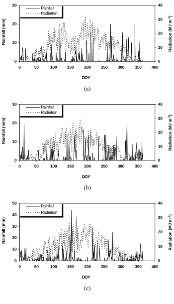
The weather data for the last 20 years (1988-2007) from a nearby weather station
which was about 25 km away from the investigated plot was analyzed to determine
the dry year, the wet year and the typical year according to yearly rainfall. The year of
1993 was found typical with yearly rainfall of 604 mm, while 1991 and 1999 were
found to be the driest and wettest with the yearly rainfall of 462 mm and 770 mm. We,
therefore, used the whole year weather data of 1991, 1993 and 1999 for the
simulations (Fig. 1). The soil water characteristics were determined using a PTFs
approach proposed by Wösten et al (1999), based on the measured soil particle
distributions and an assumed bulk density of 1.4 g cm3 for the sandy loam soil. We considered the proposed functions for estimating soil water characteristics were
particularly suitable for the case, as the published work was specifically targeting the
European soils. Table 4 shows the soil water characteristics derived using the PTFs
approach for the topsoil and subsoil. The planting and harvest dates were 1 April and
1
2
3
4
5
6
7
8
9
10
11
12
13
14
15
16
17
18
19
20
21
22
23
24
25
take up water from a saturated zone due to lack of oxygen, we considered for scenario
S1, i.e. before the motorway construction, the maximum rooting depth was restricted
to 65 cm, the average groundwater table. The upper boundary was subject to
atmospheric conditions in all the simulations. The soil water content was at its
saturation below 65 cm throughout for S1 and free drainage condition was set at the
lower boundary (2 m below the surface) for S2 as the groundwater table was far
below 2 m (estimated 4 to 5 m). The model ran from 1 January when the soil water
content was at its field capacity.
The crop parameters for root growth and root length distribution down the profile, and
the small time step for calculating evaporation, root water uptake and soil water
redistribution were set the same as those in the validation cases. In the very early crop
development stage, the model assumed a constant rooting depth of 0.2 m for the
cumulative effective day degree less than 100 d oC. The parameter values used for estimating potential soil evaporation and crop transpiration were determined
according to Allen et al. (1998).
6. Results and discussion
6.1. Model Validation
6.1.1. Model overall performance
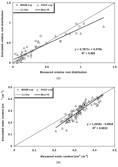
To evaluate the overall performance of the model, all the measurements collected
content in different soil layers were compared with the simulations (Fig. 2). Simulated
values of relative root density down the profile at intervals for both the Bouwing and
the PAGV experiments were not only highly correlated but almost proportional to the
measured values (Fig. 2a). Both RMSE and ME were small, only 0.1258 and 0.0016,
respectively (Table 6). This indicates that the model gave good predictions of root
dynamics during crop growth. The simulated values of soil water content also agreed
well with the measured values (Fig. 2b). Regression of simulated and measured gave a
high R 1
2
3
4
5
6
7
8
9
10
11
12
13
14
15
16
17
18
19
20
21
22
23
24
25
2 of 0.801. And again the values of RMSE (0.0412 cm3 cm-3) and ME (0.0260
cm3 cm-3) were small. Over the 99 comparisons only 22 differed by more than 0.05 cm3 cm-3 and 2 by more than 0.1 cm3 cm-3. The overall agreement between measurement and simulation for both relative root length distribution and soil water
content in various layers was good. This suggests that the model performed
reasonably well in predicting root and water dynamics in the crop-soil system. Thus
the proposed model using relatively simple algorithms has the potential to be adopted
in the agro-hydrological models for irrigation, fertilizer and pesticide practices.
6.1.2. Rooting depth and relative root length distribution
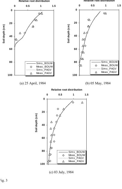
Relative root distributions down the soil profile at intervals were simulated and
compared with the measurements (Fig. 3). Generally, the model was satisfactory in
modeling root dynamics since the agreement between the simulated and measured
relative root distributions was good, indicating that the proposed equations describing
root growth and parameterization were appropriate for wheat. The difference in the
measured relative root distribution between the BOWU and the PAGV experiments
1
2
3
4
5
6
7
8
9
10
11
12
13
14
15
16
17
18
19
20
21
22
23
24
25
could not be reproduced by the model in the study since the model did not consider
the effect of soil texture on root growth. The comparison also reveals that the model
performed better in predicting relative root length distribution for the crop in the early
development stages. The measured root length distribution was well simulated on 25
April, 1984 (Fig. 3a), while the simulated root distributions at later dates deviated
from the measurements (Fig. 3bc). In the top 10 cm soil layer the model
underestimated the relative root length, whereas the opposite was found to be the case
in the 10 – 60 cm soil region. The probable reasons for the difference might be due to
the fact that soil water content was not considered in the simulation of root growth, or
that the relative root length distribution is dependent on crop development stage, and
thus underlines the possibility to further improve the root model in the future.
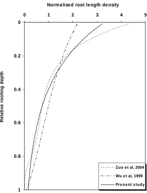
Comparison of the simulated wheat relative root length distribution in the study with
these calculated using available equations (Wu et al., 1999; Zuo et al., 2004) were
also carried out (Fig. 4). Zuo et al. (2004) described the root length distribution with a
highly non-linear equation with four parameters, while Wu et al. (1999) formulated
the distribution with a third-order polynomial equation. It was found that the modeled
relative root length distribution in the study was in good agreement with these
calculated by Wu et al. (1999) and Zuo et al. (2004) (Fig. 4). In the top and bottom
20% rooting depth the modeled root length distribution in the study was in between
those calculated by the equations proposed by Wu et al. (1999) and Zuo et al. (2004),
whereas in the middle 60% rooted region, our prediction was close to that by Zuo et al.
(2004). Both equations derived by Wu et al. (1999) and Zuo et al. (2004) were based
on comprehensive datasets made up from measurements. This indicates that the
1
2
3
4
5
6
7
8
9
10
11
12
13
14
15
16
17
18
19
20
21
22
23
24
25
distribution in the soil for wheat. This, together with the ability of modeling rooting
depth, makes the algorithm for root growth reliable for modeling water and nutrient
dynamics in wheat-soil systems.
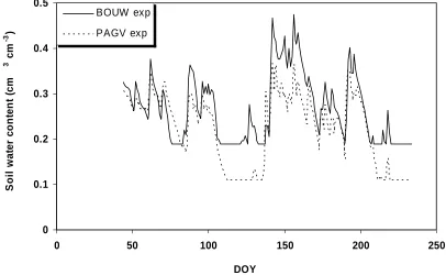
6.1.3. Soil water content in various layers
Soil water contents in 20 cm layers to 1 m were generally well simulated over time for
both experiments (Fig. 5). The model not only reproduced the patterns of soil water
changes in layers, but also produced values close to the measurements. In the top 20
cm layer, soil water content was markedly affected by rainfall. The peaks of soil water
were all coincided with big rainfall events. In the 20-40 cm layer soil water content
was less affected by rainfall. There was only one noticeable soil water increase in this
layer between Day 142 to Day 184 when big rainfall events concentrated. In the soil
layers below 40 cm, rainfall had virtually no direct influence on soil water content.
Soil water in these layers decreased constantly due to root water uptake. Despite good
overall agreement of soil water content between measurement and simulation, the
discrepancies between measured and simulated values were more evident in the 20-40
cm soil layer in the Bouwing experiment and in the top 20 cm soil layer in the PAGV
experiment. One possible reason for these discrepancies is inaccurate soil water
properties used in the simulation for these two soil layers. The measured or derived
soil water properties based on certain approaches might not be representative for the
soil at a field scale. Such a phenomenon has been encountered often and reported
previously (Hopmans and Šimunek, 1999; Ritter et al., 2003).
1
2
3
4
5
6
7
8
9
10
11
12
13
14
15
16
17
18
19
20
21
22
23
24
25
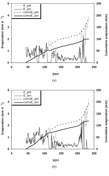
High potential soil evaporation occurred before Day 140 and after Day 205 when the
crop was at its early development stages and at its late development stage (Fig. 6). In
these stages the ground cover was less intense and therefore the evaporation demand
was larger. There were two periods from Day 110 to 138 and after Day 205 when the
actual evaporation was far less than the potential for the most days. This can be
explained by sparse rainfall during these periods and the resulting low soil water
content close to the permanent wilting point in the top 5 cm layer (Fig. 7) in both
experiments. In the rest growing period soil evaporation was basically met in both
experiments. This is because the soils in the top 5 cm layer in these periods were
relatively wet in both experiments (Fig. 7).
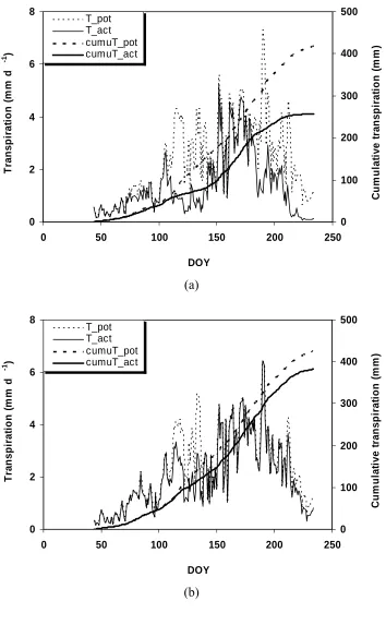
Contrary to soil evaporation, the biggest crop transpiration demand happened during
Day 140 to Day 205 when the crop was at its mid-season development stage (Fig. 8).
Wheat grown in the Bouwing experiment suffered from water stress as the cumulative
actual transpiration was clearly less than the potential one, while the crop in the
PAGV experiment was basically free from water stress (Fig. 8). The cumulative
potential transpirations for the Bouwing and the PVGA experiments were 419 and
425 mm, respectively, similar to each other. At the end of the simulation the crop in
the Bouwing experiment was only able to extract 257 mm water from the soil,
whereas the corresponding value for the PAGV experiment was 383 mm. In the
Bouwing experiment water stress occurred mainly in two periods, i.e. Day 108 to Day
145 and after Day 205 when the potential transpiration clearly exceeded the actual one
(Fig. 8a), resulting from low water content in the top 20 cm and 20-40 cm layers (Fig.
1
2
3
4
5
6
7
8
9
10
11
12
13
14
15
16
17
18
19
20
21
22
23
24
25
happened only in a brief period between Day 115 to Day 138. This contrasting
difference between two experiments was primarily caused by a free drainage in the
100-120 cm layer in the Bouwing experiment, which made the soil water flow
upwards impossible from below 120 cm, and the relatively high groundwater table in
the PAGV experiment, which made more water available for roots to take up in the
lower soil region due to capillary flow.
It should be pointed out that due to the small time step employed in calculating soil
evaporation, crop transpiration and soil water movement, the model is flexible to use
the weather information collected at shorter intervals, say hourly, to produce more
accurate results. The disadvantage is that it takes longer to run the model compared to
other approaches. However the computation effort is quite affordable with modern
computing equipment. For the cases above it only took a personal PC with a pentium
IV processor about 35 seconds CPU time to run each case.
6.2. Model application
The potential and actual cumulative crop transpirations over the growing period from
1 April to 1 October in the dry, the typical and the wet years were simulated for the
application case with Brussels sprouts (Fig. 9). The calculated potential cumulative
transpiration during growth was 430 mm in the typical year, similar with the values of
441 mm and 420 mm for the dry year and the wet year. The simulations for Scenario
S1 in all three different years, i.e. before the motorway construction, show that the
crop was basically able to extract water from the soil to meet potential transpiration
1
2
3
4
5
6
7
8
9
10
11
12
13
14
15
16
17
18
19
20
21
22
23
24
25
due to lowering the groundwater table resulting from the motorway construction.
Without irrigation, the crop was only capable of taking up about 160 mm from the soil
in the typical year. Likewise the values are 130 mm and 200 mm for the dry year and
the wet year, respectively. The reduction in transpiration was caused by the lack of
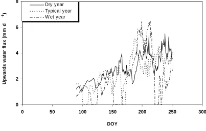
water supply from groundwater. Simulations reveal there was no upwards capillary
water flow at the depth of 50 cm from the surface in S2, whilst a substantial water
supply at this depth from groundwater was simulated in S1, and the supply tended to
increase with time despite the fluctuations (Fig. 10). The variations of soil water
content in different soil layers for both scenarios were also simulated (data not shown).
In the top 0-30 cm soil layers, the water content was heavily influenced by rainfall as
found in the validation cases. It appears that the influence was limited in the top 30
cm region, since the changes in water content in the soil below was not correlated
with rainfall. Also it is clear that the water content in different soil layers in S2 was
constantly lower than that in S1 during the growing period.
From the above it can be concluded that the construction of a motorway has a serious
negative effect on the ability of a crop to take up water from the soil without irrigation.
Since crop transpiration is positively related to the crop yield (Wild, 1988; Allen et al.,
1998), the significant reduction in transpiration will inevitably lead to a reduction in
yield.
7. Conclusions
An easy-to-use procedure, using an integrated Richards equation solution for soil
1
2
3
4
5
6
7
8
9
10
11
12
13
14
15
16
17
18
19
20
21
22
23
24
the small time step employed in the model, the coupled processes of soil evaporation,
crop transpiration and soil water movement were successfully decoupled, leading to
simple algorithms that are easily implemented. Thus the complex numerical schemes
and associated long program codes for accurate simulation of water dynamics in the
crop-soil system are avoided, which makes it easier to use the basic theory of soil
water flow in the agro-hydrological models. Further, the small time step makes it
possible to use the weather information collected at any time intervals. The validation
of the model against data from field experiments on two contrasting soils cropped
with wheat showed that the model was capable of making good predictions of soil
water content at different depths and at intervals during crop growth. This proves that
the proposed algorithms for modeling water dynamics in various processes in the
crop-soil system were reasonable and the model was adequately constructed. Since
the model is simple and sufficiently accurate for the simulations at a field scale, it has
the potential to be employed in agro-hydrological models for irrigation, fertilizer and
pesticide practices.
Finally it is worth pointing out that the model developed in the study is a deterministic
one which works well when all the input parameters are known with certainty. To
further extend the model for prediction purposes, consideration of dealing with
parameters with stochastic nature such as rainfall should be made in the future (Laio,
2006).
1
2
3
4
5
6
7
8
9
10
11
12
13
14
15
16
17
18
19
20
21
22
23
24
The work was partly financed by the UK Department for Environment, Food and
Rural Affairs through the project HH3507SFV. The authors gratefully thank Dr J
Neeteson for kindly providing the essential dataset for validating the model proposed
in the study. D Yang acknowledges the financial support from the China Scholarship
Council for his joint PhD program between Zhejiang University, China, and Warwick
University, UK.
References
Allen R.G., Pereira L.S., Raes D., Smith, M., 1998. Crop evapotranspiration.
Guidelines for computing crop water requirements. FAO Irrigation and Drainage
Paper 56. FAO, Rome.
Arnold J.G., Allen P.M., Bernhardt G.T., 1993. A comprehensive
surface-groundwater flow model. J. Hydrol. 142, 47-69.
Aydin M., Yang S.L., Kurt N., Yano T., 2005. Test of a simple model for estimating
evaporation from bare soils in different environments. Ecol. Model. 182, 91-105.
Bastiaanssen W.G.M., Allen R.G., Droogers P., D’Urso G., Steduto P., 2007.
Twenty-five years modeling irrigated and drained soils: State of the art. Agr. Water
Manage. 92, 111-125.
Bitterlich S., Durner W., Iden S.C., Knabner P., 2004. Inverse estimation of the
unsaturated soil hydraulic properties from column outflow experiments using
free-form parameterization. Vadose Zone J. 3, 971-981.
Bohne K., Salzmann W., 2002. Inverse simulation of non-steady-state evaporation
1
2
3
4
5
6
7
8
9
10
11
12
13
14
15
16
17
18
19
20
21
22
23
24
25
Boone A., Wetzel P.J., 1996. Issues related to low resolution modeling of soil
moisture: Experience with the PLACE model. Global Planet. Change 13, 161-181.
Brisson N., Gary C., Justes E., Roche D., Zimmer D., Sierra J., Bertuzzi P., Burger P.,
Bussière F., Cabidoche Y.M., Cellier P., Debaeke P., Gaudillère J.P., Hénault C.,
Maraux F., Seguin B., Sinoquet H., 2003. An overview of the crop model STICS.
Eur. J. Agron. 18, 309-332.
Cresswell H.P., Coquet Y., Bruand A., McKenzie N.J., 2006. The transferability of
Australian pedotransfer functions for predicting water retention characteristics of
French soils. Soil Use Manage. 22, 62-70.
De Willigen P., 1991. Nitrogen turnover in the soil-crop system; comparison of
fourteen simulation models. Fert. Res. 27, 141-149.
Droogers P., Tobari M., Akbari M., Pazira E., 2001. Field-scale modeling to explore
salinity problems in irrigated agriculture. Irrig. Drain. 50, 77-90.
Feddes R.A., Kowalik P.J., Zaradny H., 1978. Water uptake by plant roots. In: Feddes
R.A., Kowalik P.J., Zaradny H. (Eds.), Simulation of Field Water Use and Crop
Yield. John Wiley & Sons, Inc., New York.
Gerwitz A., Page E.R., 1974. Empirical mathematical - model to describe plant root
systems 1. J. Appl. Ecol. 11, 773-781.
Greenwood D.J., 2001. Modelling N-response of field vegetable crops grown under
diverse conditions with N_ABLE: A review. J. Plant Nutr. 24, 1799-1815.
Groot J.J.R., Verberne E.L.J., 1991. Response of wheat to nitrogen fertilization, a data
set to validate simulation models for nitrogen dynamics in crop and soil. Fert. Res.
27, 349-383.
Hopmans J.H., Šimunek J., 1999. Review of inverse estimation of soil hydraulic
1
2
and Measurement of the Hydraulic Properties of Unsaturated Porous Media.
University of California, CA, pp. 634-659.
3
4
5
6
7
8
9
10
11
12
13
14
15
16
17
18
19
20
21
22
23
24
http://www.fao.org/nr/water/infores_databases_cropwat.html.
Hu K., Li B., Chen D., Zhang Y., Edis R., 2008. Simulation of nitrate leaching under
irrigated maize on sandy soil in desert oasis in Inner Mongolia, China. Agri.
Water Manage. 95, 1180-1188.
Huyer W., Neumaier A., 1999. Global optimization by multilevel coordinator search.
J. Global Optim.14, 331-355.
Hwang S.II., Powers S.E., 2003. Using particle-size distribution models to estimate
soil hydraulic properties. Soil Sci. Soc. Am. J. 67, 1103-1112.
Ines A.V.M., Droogers P., 2002. Inverse modeling in estimating soil hydraulic
functions: a Genetic Algorithm approach. Hydrol. Earth Syst. Sci. 6, 49-65.
Jhorar R.K., Bastiaanssen W.G.M., Feddes R.A., Van Dam J.C., 2002. Inversely
estimating soil hydraulic functions using evapotranspiration fluxes, J. Hydrol. 258,
198-213.
Jiménez-Martínez J., Skaggs T.H., van Genuchten M.Th., Candela L., 2009. A root
zone modelling approach to estimating groundwater recharge from irrigated areas.
J. Hydrol., doi:10.1016/j.jhydrol.2009.01.002
Kage H., Kochler M., Stutzel H., 2000. Root growth of cauliflower (Brassica
oleracea L. botrytis) under unstressed conditions: measurement and modelling.
Plant Soil 223, 131-145.
Kirby J.M., Ringrose-Voase A.J., 2000. Drying of some Philippine and Indonesian
puddle rice soils following surface drainage: numerical analysis using a swelling
1
2
3
4
5
6
7
8
9
10
11
12
13
14
15
16
17
18
19
20
21
22
23
24
Kristensen H.L., Thorup-Kristensen K., 2004. Uptake of 15N labeled nitrate by root
systems of sweet corn, carrot and white cabbage from 0.2 to 2.5 m depth. Plant
Soil 265, 93-100.
Lee D.H., Abriola L.M., 1999. Use of the Richards equation in land surface
parameterizations. J. Geophys. Res. 104, 27519-27526.
Laio F., 2006. A vertically extended stochastic model of soil moisture in the root zone.
Water Resour. Res. 42, W02406.
Merdum H., Cinar O., Meral R., Apan M., 2006. Comparison of artificial neural
network and regression pedotransfer functions for prediction of soil water
retention and saturated hydraulic conductivity. Soil Till. Res. 90, 108-116.
Minasny B., Field D.J., 2005. Estimating soil hydraulic properties and their
uncertainty: the use of stochastic simulation in the inverse modelling of the
evaporation method. Geoderma 126, 277-290.
Montaldo N., Rondena R., Albertson J.D., Mancini M., 2005. Parsimonious modeling
of vegetation dynamics for ecohydrologic studies of water-limited ecosystems.
Water Resour. Res. 41, W10416.
Mualem Y., 1976. A new model for predicting the hydraulic conductivity of
unsaturated porous media. Water Resour. Res. 12, 513-522.
Pedersen A., Zhang K., Thorup-Kristensen K., Jensen L.S., 2007. Simulating root
density dynamics and nitrogen uptake – Is a Simple Approach Sufficient? 37th Biological Systems Simulation Conference, 17-19 April, 2007, Maryland, U.S.A.
Rahn C.R., Zhang K., Lillywhite R., Ramos C., Doltra J., de Paz J. M., Riley H., Fink
M., Nendel C., Thorup-Kristensen K., Piro F., Venezia A., Firth C., Schmutz U.,
the economic output and environmental benefits on cropping rotations. 16th
International CIEC symposium, 16-19 September, Gent, Belgium. 1
2
3
4
5
6
7
8
9
10
11
12
13
14
15
16
17
18
19
20
21
22
23
24
Renaud F.G., Bellamy P.H., Brown C.D., 2008. Simulation pesticides in ditches to
asses ecological risk (SPIDER): I. Model description. Sci. Total Environ. 394,
112-123.
Ritchie J.T., 1998. Soil water balance and plant water stress. In: Tsuji G.Y. et al. (Eds),
Understanding Options for Agricultural Production, pp. 41-54.
Ritter A., Hupet F., Munoz-Carpena R., Lambot S., Vanclooster M., 2003. Using
inverse methods for estimating soil hydraulic properties from field data as an
alternative to direct methods. Agr. Water Manage. 59, 77-96.
Schmitz G.H., Puhlmann H., Droge W., Lennartz. F., 2005. Artificial neural networks
for estimating soil hydraulic parameters from dynamic flow experiments. Eur. J.
Soil Sci. 56, 19-30.
Šimunek J., Vogel T., Van Genuchten M.Th., 1992. The SWMS_2D code for
simulating water flow and solute transport in two-dimensional variably saturated
media, v 1.1, Research Report No. 126, U. S. Salinity Lab, ARS USDA, Riverside.
Sonnleitner M.A., Abbaspour K.C., Schulin R., 2003. Hydraulic and transport
properties of the plant–soil systems estimated y inverse modelling. Eur. J. Soil Sci.
54, 127-138.
Thorup-Kristensen K., 2006. Root growth and nitrogen uptake of carrot, early
cabbage, onion and lettuce following a range of green manures. Soil Use Manage.
22, 29-38.
Van Genuchten M.Th., 1980. A closed-form equation for predicting the hydraulic
1
2
3
4
5
6
7
8
9
10
11
12
13
14
15
16
Van Genuchten M.Th., Leij F.J., Yates S.R., 1991. The RETC code for quantifying
the hydraulic functions of unsaturated soils. Robert S. Kerr Environmental
Research Laboratory, U. S. Environmental Protection Agency, Oklahoma, USA,
83pp.
Wild A. (Ed.), 1988. Russell’s Soil Conditions and Plant Growth. Longmans
Scientific and Technical.
Wösten J.H.M., Lilly A., Nemes A., Le Bas C., 1999. Development and use of a
database of hydraulic properties of European soils. Geoderma 90, 169-185.
Wu J., Zhang R., Gui S., 1999. Modeling soil water movement with water uptake by
roots. Plant Soil 215, 7-17.
Zhang K., Greenwood D.J., White P.J., Burns I.G., 2007. A dynamic model for the
combined effects of N, P and K fertilizers on yield and mineral composition;
description and experimental test. Plant Soil 298, 81-98.
Zuo Q., Jie F., Zhang R., Meng L. 2004, A generalized function of wheat’s root length
Figure captions:
1
2
3
4
5
6
7
8
9
10
11
12
13
14
15
16
17
18
19
20
21
22
23
24
Figure 1: Rainfall and radiation distributions used in the simulations for the dry year
(a), the typical year (b) and the wet year (c) in the application case.
Figure 2: Overall comparison of relative root density distribution at interval (a) and
soil water content in various soil layers (b) between measurement and
simulation for the Bouwing and the PAGV experiments.
Figure 3: Comparison of relative root distribution between measurement and
simulation at intervals of the Bouwing and the PAGV experiments.
Figure 4: Comparison of distribution of normalised root length density proposed in
the study with these calculated from literature for wheat.
Figure 5: Comparison between the measured and simulated volumetric soil water
content at different soil layers for the Bouwing experiment (a) and the
PAGV experiment (b).
Figure 6: Daily and cumulative potential and actual evaporation for the Bouwing
experiment (a) and the PAGV experiment.
Figure 7: Variations of soil water content in the top 5 cm soil layer for both the
wilting point in the top 5 cm soil layer for the Bouwing and PAGV
experiments are 0.169 and 0.114 cm 1
2
3
4
5
6
7
8
9
10
11
12
13
14
3 cm-3, respectively).
Figure 8: Daily and cumulative potential and actual transpiration for the Bouwing
experiment (a) for the PAGV experiment (b).
Figure 9: Simulated potential and actual cumulative transpiration during growth for
scenarios of S1 (before construction) and S2 (after construction) in the dry
year (a), the typical year (b) and the wet year (c).
Figure 10: Simulated upwards water flux at 50 cm below the soil surface during
growth for scenarios of S1 (before motorway construction) and S2 (after
Table captions:
1
2
3
4
5
6
7
8
9
10
11
12
13
14
15
16
17
18
19
20
Table 1: van Genuchten parameter values in Eqs. (2) and (3) for coarse, medium and
fine soils (Wösten et al., 1999)
Table 2: Summary of the Bouwing and the PAGV experiments
Table 3: Monthly average rainfall and mean air temperature in the application case
Table 4: Measured particle size distribution and soil organic matter, and soil hydraulic
properties derived using PTFs proposed by Wösten et al. (1999) for the
topsoil (0 – 45 cm) and subsoil (45 – 100 cm) in the application case
Table 5: Fitted van Genuchten parameter values in Eq. (12) for the Bouwing and the
PAGV experiments using the RETC software (van Genuchten et al., 1991)
Table 6: Statistical comparisons between measurement and simulation of relative root
length distribution and soil water content in various layers for both the
0 10 20 30
0 50 100 150 200 250 300 350 400
DOY R a in fa ll ( m m ) 0 10 20 30 40 R ad iat io n ( M J m -2) Rainfall Radiation (a) 0 10 20 30
0 50 100 150 200 250 300 350 400
DOY R a in fa ll ( m m ) 0 10 20 30 40 R ad iat io n ( M J m -2) Rainfall Radiation (b) 0 10 20 30 40 50
0 50 100 150 200 250 300 350 400
[image:40.595.122.472.100.710.2]