Technical analysis and central bank intervention

WORKING PAPERS SERIES

WP99-04

Technical Analysis and Central Bank

Intervention

Federal Reserve Bank of St. Louis

TECHNICAL ANALYSIS AND CENTRAL BANK INTERVENTION -- By Christopher Neely and Paul Weller

ABSTRACT --97-002B

Technical Analysis and Central Bank Intervention

Christopher J. Neely*

Paul Weller†

Revised version: March 26, 1999

Keywords: technical trading rules, genetic programming, exchange rates, central bank intervention

JEL subject numbers: F31, G15

* Senior Economist, Research Department Federal Reserve Bank of St. Louis P.O. Box 442 St. Louis, MO 63166 (314) 444-8568, (314) 444-8731 (fax)

[email protected]

† Department of Finance

Henry B. Tippie College of Business Administration University of Iowa

Iowa City, IA 52242

(319) 335-1017, (319) 335-3690 (fax)

[email protected]

The authors would like to thank Robert Dittmar for excellent programming assistance, Kent Koch for excellent research assistance, Owen Humpage for helpful comments on an earlier draft and their colleagues at the Federal Reserve Bank of St. Louis for generously sharing their computers at night and over

Introduction

There is now a considerable amount of evidence to suggest that technical trading

rules can earn economically significant excess returns in the foreign exchange market

(Dooley and Shafer, 1984; Levich and Thomas, 1993; Neely, Weller and Dittmar, 1997

(henceforth NWD); Neely and Weller, 1998; Sweeney, 1986). But the reasons for the

existence of these excess returns are still not well understood. One possible explanation is

that the intervention activities of central banks in the market may account for at least part

of the profitability of technical trading rules (Dooley and Shafer, 1984; LeBaron, 1998;

Szakmary and Mathur, 1997; Neely, 1998). The arguments advanced in favor of this

hypothesis focus on the fact that central banks are not profit maximizers, but have other

objectives that may make them willing to take losses on their trading. Thus, the stated

goal of intervention by the Federal Reserve is to maintain orderly market conditions, and

the unstated goals may include the achievement of macroeconomic objectives such as

price stability or full employment. If the target for the exchange rate implied by these

goals is inconsistent with the market’s expectations of future movements in the exchange

rate, there may be an opportunity for speculators to profit from the short-run fluctuations

introduced (Bhattacharya and Weller, 1997).

LeBaron (1998) investigated the relationship between intervention by the Federal

Reserve and returns to a simple moving average trading rule. He used daily intervention

data to show that most excess returns were generated on the day before intervention

occurred. He found that removing returns on the days prior to U.S. intervention reduced

the trading rule excess returns to insignificance. Szakmary and Mathur (1997) examined

exchange reserves—a proxy for intervention—of five central banks. They also found

evidence of an association between intervention activity and trading rule returns.

The fact that trading rule returns were abnormally high on the day before

intervention tends to support the hypothesis that strong and predictable trends in the

foreign exchange market cause intervention, rather than that intervention generates

profits for technical traders. But it still leaves open the possibility that a sophisticated

technical trader might be able to respond to the fact that intervention had occurred to

modify his position and increase his profits. If this is the case, then observing intervention

carries additional useful information about the future path of the exchange rate that is not

contained in current and past rates.

Thus we are interested in determining whether knowledge of central bank

intervention can increase excess returns to trading rules in dollar exchange rate markets.

We investigate this question using the methodology developed in NWD (1997). This

allows us to identify optimal ex ante trading rules that use information about whether

intervention has occurred, and to compare their profitability to that of rules obtained

without the use of such information. We find substantial differences between in-sample

and out-of-sample periods, suggesting that the effects of intervention have not been stable

over time. We also find strong evidence for two currencies (British pound and Swiss

franc) that the use of in-sample intervention data improves the efficiency with which

1. Methodology

We use genetic programming as a search procedure to identify trading rules that

use information both on the past exchange rate series and on intervention activity. We

have previously used this technique to find profitable rules that use data on exchange

rates alone (NWD, 1997) and exchange rates and interest rates (Neely and Weller, 1998).

It has also been applied in the equity market (Allen and Karjalainen, 1998). The method

is particularly useful for our purposes as it permits flexible incorporation of additional

information on central bank intervention into the trading rule.

The genetic program operates by creating successive populations of trading rules

according to certain well-defined procedures. Profitable rules are more likely to have

their components reproduced in subsequent populations. The basic features of the genetic

program are: (a) a means of encoding trading rules so that they can be built up from

separate subcomponents; (b) a measure of profitability or “fitness”; (c) an operation

which splits and recombines existing rules in order to create new rules.

Before we describe these features, let us first introduce some notation. The

exchange rate at date t (USD per unit of foreign currency) is given by S_t. Intervention at date t is given by the indicator variable, I_t, which can take on values 1, 2, or 3, according to whether the U.S. authorities buy dollars, do not intervene, or sell dollars respectively at

date t. A trading rule can be thought of as a mapping from past exchange rates and intervention data to a binary variable, z_t, which takes the value +1 for a long position in foreign exchange at time t, and -1 for a short position. Trading rules may be represented as trees, whose nodes consist of various mathematical functions, logical operators and

“lag”. The functions are distinguished by the data series on which they operate. Thus

maxS(k) is equivalent to max

(

)

operators include “and”, “or”, “not”, “if-then” and “if-then-else”.

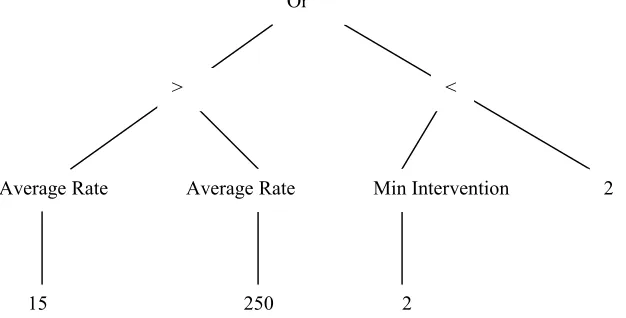
Figure 1 presents an example of a simple trading rule that makes use of both

exchange rate and intervention data. It signals a long position in foreign currency at date t

if the 15-day moving average is greater than the 250-day moving average, or if the U.S.

authorities intervened to buy dollars in the last two days, otherwise a short position.

The fitness criterion we use in the genetic program is the excess return to a fully

margined long or short position in the foreign currency. The continuously compounded

(log) excess overnight return is given by ztrt where zt is the indicator variable described

above, and rt is defined as:

r_t =lnS_t+ !lnS_t +ln( +i_t ) ln(! +i_t)

*

1 1 1 .

(1)

The domestic (foreign) overnight interest rate is i_t (i_t*_{). The cumulative excess return}

from two round-trip trades1 (go long at date t, go short at date t + k), with round-trip proportional transaction cost c, is

r_{t t k} r_{t i} c c

i k

,+ + ln( ) ln( )

=

!

=

_"

0 1

1 1

(2)

Therefore the cumulative excess return r for a trading rule giving signal zt at time t over

the period from time zero to time T is:

1 _{Each trade incurs a round-trip transaction cost because it involves closing a long (short)}

# $ % & ' ( + ! + =

_"

where n is the number of trades. This measures the fitness of the rule.

To implement the genetic programming procedures we define 3 separate

subsamples, the training, selection and validation periods. The first two periods are

equivalent to an in-sample estimation period. The third, the validation period, is used to

test the rules trained and selected in the first two periods. The results from this period

therefore constitute a true out-of-sample test of the performance of the rules. The distinct

time periods for all currencies were chosen as follows: training period, 1975-1977;

selection period, 1978-1980; validation period, 1981-1996.

The separate steps involved in implementing the genetic program are described

below.

Step 1. Create an initial generation of 500 randomly generated rules.

Step 2. Measure the excess return of each rule over the training period and rank according to excess return.

Step 3. Select the highest ranked rule and calculate its excess return over the selection period. If this rule generates a positive excess return, save it as the initial best rule. Otherwise, designate the no-trade rule as the initial best rule, with zero excess return.

Step 4. Select two rules at random from the initial generation, using weights attaching higher probability to more highly-ranked rules. Apply the recombination operator to

create a new rule, which then replaces an old rule, chosen using weights attaching higher

probability to less highly-ranked rules. Repeat this procedure 500 times to create a new

Step 5. Measure the fitness of each rule in the new generation over the training period. Take the best rule in the training period and measure its fitness over the selection period.

If this best-of-generation rule outperforms the previous best rule, save it as the new best

rule.

Step 6. Return to step 4 and repeat until we have produced 50 generations or until no new best rule appears for 25 generations.

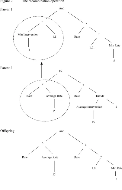
The stages above describe one trial. Each trial produces one rule whose performance is assessed by running it over the validation period from 1981-1996. Figure

2 illustrates the splitting and recombination operation referred to in Step 4. A pair of rules

is selected at random from a population, with a probability weighted in favor of rules

with higher fitness. Then subtrees of the two parent rules are selected randomly. One of

the selected subtrees is discarded, and replaced by the other subtree, to produce the

offspring rule.2

The round-trip transaction cost c was set to 0.0005 (5 basis points) in the validation period to reflect accurately the costs to a large institutional trader.3 In the

training and selection periods, however, we treat c as a parameter in the search algorithm and set it equal to 0.001 to bias the search in favor of rules that trade less frequently. We

have shown in NWD (1997) that this is an effective way of reducing the chances of

overfitting the data.

2 _{The operation is carried out subject to the requirement that the resulting rule must be}

2. The Data

We use the noon (New York time) buying rates for the German mark, yen, pound

sterling and Swiss franc (USD/DEM, USD/JPY, USD/GBP, and USD/CHF) from the

H.10 Federal Reserve Statistical Release. Daily interest rate data are from the Bank of

International Settlements (BIS), collected at 9:00am GMT (4:00am, New York time).

As in NWD (1997), we normalize the exchange rate data by dividing by a

250-day moving average. The intervention data we use is the “in market” series from the

Federal Reserve Board aggregated across all currencies. The “in market” transactions are

explicitly conducted to influence the exchange rate. We construct a variable that can take

on one of three values, 1, 2 or 3, depending on whether the U.S. authorities bought

dollars, did not transact, or sold dollars on a particular day.

Table 1 presents some summary statistics for the various exchange rate returns,

including the interest differential but excluding interest accruing over weekends and other

missing observations. There is little evidence of significant skewness, and all return series

are strongly leptokurtic. Table 2 provides summary statistics on U.S. intervention. We see

that the frequency of intervention has declined dramatically over time. Dollar purchases

were seven times more frequent during the selection period than the validation period.

This partly reflects the fact that from 1981 to 1985 there was very little intervention by

the United States.4 There has also been relatively little intervention during the Clinton

administration. At the same time the mean size of intervention has increased by a similar

order of magnitude. The average dollar purchase was eleven times greater in the

3 _{NWD (1997) discuss estimates of transaction costs.}

4 _{This was the result of a conscious policy decision by the Reagan administration (see the}

validation period than in the training period. In Table 3 we show the breakdown of

intervention in different currencies over the different sample periods. The DEM has been

the dominant intervention currency throughout the sample period, but the JPY is much

more commonly used during the validation period. Although there were no JPY

interventions at all during the training period, the currency accounted for 45 per cent of

intervention volume during the validation period. There is a correspondingly sharp

decline in the volume of intervention in other currencies during this period.

3. Results

3.1 Granger Causality

To provide a benchmark against which to interpret our results, we first analyze

two two-variable vector autoregressions run on the full sample of data from 1981 to

1996. The first includes the exchange rate return and the quantity of intervention by the

Federal Reserve, and the second substitutes for the simple return the squared exchange

rate return as a measure of volatility. The Akaike information criterion selected 16-23

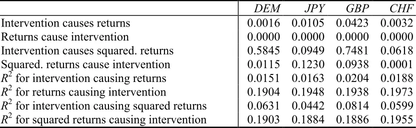
lags for each of the eight systems. The p-values reported in Table 4 indicate the

probability that we would obtain at least as extreme a test statistic if there were no

Granger causality. Thus a low p-value provides support for the presence of causality.

There is very strong evidence that returns and squared returns (except for the JPY) help

predict intervention and also support for the hypothesis that intervention causes returns.

If intervention is a predictor of future exchange rate returns, then observing

whether intervention has occurred may be valuable information for foreign exchange

power to predict returns does not necessarily imply that a trading strategy that conditions

on intervention will be more profitable than one that does not. There are several reasons

for this. First, Granger causality tests identify relationships of linear predictability,

whereas the genetic programming procedure is not constrained in the same way. Thus the

predictive power attributed to intervention by the Granger causality tests may also be

present as a non-linear component in the past exchange rate return series. This component

may already have already been incorporated into the trading rules trained only on

exchange rate data. Second, the causality tests use the magnitude of intervention, which is

not observed by traders in the market at the time of intervention. In contrast we provide

the genetic program with information only about whether the Federal Reserve intervened

on a particular day, and if so, on what side of the market. Third, evidence of causality

provides no indication of the economic significance of the relationship. In particular,

transactions costs may eliminate any potential increase in profitability.

3.2 Performance Comparisons

We have already shown in our earlier paper (NWD, 1997) that trading rules

identified by genetic programming and based only on past observations of the exchange

rates earn significant excess returns in the out-of-sample period. Here we compare the

performance of trading rules trained only on exchange rate data with rules trained on both

exchange rate and intervention data.5 We run 200 trials for each currency, 100 with

5 _{In NWD (1997) we used exchange rate data from DRI. In an earlier version of this}

intervention data and 100 without. This generates a set of 100 rules for each currency

under each informational scenario. We adopt this approach because the output from a

genetic program is inherently stochastic. Although successful rules should detect similar

predictive patterns in the data, there is generally some variation in the structure of rules

generated from distinct trials. We therefore need a large enough sample of rules to

produce a reliable estimate of the average difference in excess return.

The results of the comparison are displayed in Table 5. The mean improvement in

excess return over all currencies is 0.68 per cent per annum. But no consistent pattern

emerges. The return to the CHF rules improves by 3.1 per cent and to the GBP by 1.1 per

cent. But returns for the DEM and JPY are adversely affected. The improvement in

performance for the CHF is accompanied by an increase in the number of rules producing

a positive excess return from 49 to 89. It is also clear that the information on intervention

is being incorporated into the trading rules, as indicated by the substantial changes in

trading frequency and proportion of time spent in a long position. We present further

evidence on this issue below.

Although the information presented in Table 5 is a useful way of summarizing the

performance of the trading rules, it does not accurately reflect the returns that a trader

would have earned from the use of these rules. Even if a trader had chosen to attach a

weight of 1/100 to each individual rule, the mean return understates the return to this

composite rule by double counting some transaction costs. We consider two alternative

ways of aggregating the information contained in the individual rules into a composite

important, since as Peiers (1997) has shown, there are significant information asymmetries around the time of intervention, which in her study of Bundesbank

trading rule: the uniform portfolio rule and the median portfolio rule. The uniform portfolio rule allocates a fraction 1/100 of the value of the portfolio to each rule.6 The

median portfolio rule generates a long signal at date t if 50 per cent or more of the rules give a long signal at date t. Otherwise it gives a short signal. The performance of the uniform and median portfolio rules with and without intervention information is

presented in Table 6.

As might be expected from Table 5, the effects of supplying information on

intervention are mixed. In the case of the CHF there is a very substantial improvement in

the performance of both uniform and median portfolio rules. The return to the uniform

rule rises from 1.35 per cent to 4.19 per cent, and the return to the median rule rises from

–0.13 per cent to 5.36 per cent. There is also considerable improvement in the

performance of rules for the GBP, where the median portfolio return rises by 3.66 per

cent. But excess returns are adversely affected in the case of the DEM and JPY.

To test the significance of the difference between the portfolio rule returns with

and without intervention information, we report Bayesian posterior probabilities. A

probability greater than 0.5 means that the evidence favors the hypothesis that excess

returns are higher when intervention information is used. Strong evidence of an

improvement in performance exists for the CHF and GBP. However, there is also strong

evidence that the median rules for the DEM and JPY did less well with intervention data

than without.

the results with the DRI data set exaggerated the impact of intervention information on trading rule profitability.

6 _{The excess return to the uniform rule coincides exactly with the mean excess return}

3.3 How is the Intervention Data Used?

We conduct two experiments in order to illuminate the way in which the

information on intervention influences the performance of the rules. First we compute

returns to the rules that are trained with intervention data but are then supplied with a

fictitious series out-of-sample indicating that intervention is always zero. Comparing

Panel A of Table 7 with the results in Table 5 we see that performance actually improves

for the DEM and CHF, and is essentially unaffected for the JPY and GBP. This is an

indication that there has been a change in the response of the exchange rate to

intervention between in-sample and out-of-sample periods. It also demonstrates that for

the GBP and CHF, the two currencies where intervention information improved

performance, all the value of training rules with intervention data comes from more

efficient use of the information contained in the past exchange rate series alone. The

intervention signal, by changing the structure of the rules, is able to filter out the impact

of intervention.

Next we perform the following simulation experiment. We assume that a simple

Markov switching model generates the intervention series independently of the return

series. We generate 100 simulated intervention series using the transition probabilities

estimated from the validation period and run each set of 100 rules on the observed

exchange rate data and the simulated intervention series. This procedure eliminates any

predictive power that intervention might have had for future exchange rate returns. In

Panel B of Table 7 we report the performance of each set of rules. All four rules perform

more poorly, and average excess return falls by 0.93 per cent when compared to the

figures in Table 5. There is also a substantial increase in trading frequency. Evidently the

simulation procedure has eliminated features of the joint distribution of intervention and

exchange rate returns that had been incorporated into the trading rules.

The most direct method for determining how the genetic programming rules use

the central bank intervention data is to analyze the structure of individual rules. But this

approach is generally informative only when the structure of the rule to be analyzed is

fairly simple. Although such rules may not be representative of the total population, it is

interesting to examine an example of a simple rule produced for the CHF. The rule,

illustrated in Figure 3, had a mean annual excess return of 4.48 per cent per annum over

the out-of-sample period, and a correlation of 98.53 per cent with the median portfolio

rule. It provides a clear illustration of the way in which intervention information

influences the signal. The rule instructs “Take a long position in foreign currency if the

normalized exchange rate is greater than the norm (absolute value of the difference) of

the maximum value of the intervention variable (over a time window determined by

current intervention) and the normalized exchange rate.” The price normalization

(division by a 250-day moving average) means that the exchange rate series moves fairly

closely around unity. So on a date when the Federal Reserve buys dollars (I = 1) the rule will always signal a long position in foreign currency, and conversely on a day when it

sells dollars (I = 3) the rule will always signal a short position. Otherwise the rule takes a form that is essentially equivalent to “Take a long position in foreign currency if the

3.4 Trading Rule Returns around Intervention

We next turn to investigating the performance of the trading rules around days

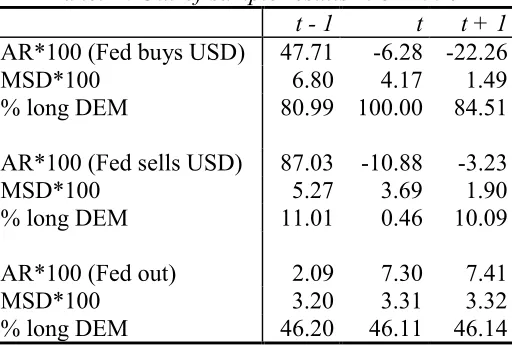
when intervention took place, concentrating on the median portfolio rules. In Panel A of

Table 8 we present for the USD/DEM the annualized daily percentage return over the

period 1981-1996, conditioned on intervention by the U.S. authorities at time t. There is an immediately striking feature to these figures. The excess return at t – 1, i.e. the return from date t – 1 to date t, is very much larger than the returns on the subsequent two days when the Fed is in the market.7 This explains why the return at t – 1 conditional on no intervention at t is significantly lower than the unconditional mean return. Many of the largest returns to the trading rule are excluded. Notice also that the intervention that

occurs at date t is on the opposite side of the market from that taken by the trading rule. The portfolio rule tends to be long in foreign currency at t – 1 when there is a large depreciation of the dollar from t – 1 to t, and this depreciation is associated with

purchases of dollars by the Federal Reserve. This clearly supports the hypothesis that the Federal Reserve intervenes to check a strong and predictable trend in the exchange rate.

Consistent with results found by Humpage (1998) the figures in the table indicate that at

least over a very short horizon the action is successful during the period 1981-96. From

the top row we see that if the Federal Reserve intervened and bought dollars at date t, the return to the median portfolio rule from t to t + 2 was –29 per cent. Since the great majority of individual rules took a long position in foreign currency, this indicates on

average an appreciation of the dollar on this date. A similar picture emerges for dollar

7 _{These results are consistent with LeBaron (1998), who found that removing returns on}

sales. The return to the USD/DEM rule was 87 per cent at t – 1, and – 14 per cent over the subsequent two trading days.

In Panel B we present the same calculations for the period 1975-1980.8 The

pattern of returns is rather different. Returns to trading rules taking the opposite side of

the market continue to be positive on the day following an intervention. This indicates

that there was a change in the response of the exchange rate to intervention between

in-sample and out-of-in-sample periods. It is clear that the DEM trading rules correctly

identified a profitable reaction to intervention over the period 1975-1980. However, this

reaction was no longer profitable over the period 1981-1996. This change in the impact

of intervention provides us with an explanation for the somewhat poorer out-of-sample

performance of the trading rules using intervention information compared to those using

only exchange rate information.

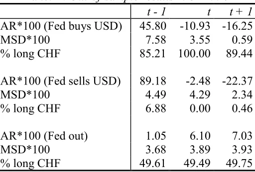
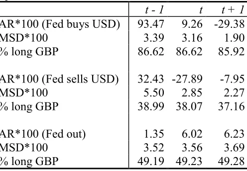
We see the same effect at work in the case of the CHF and GBP in Tables 9 and

10. It is striking that here despite the altered reaction of the exchange rate to intervention

in the out-of-sample period, training with intervention data still produced an overall

improvement in performance. The results for the JPY are not informative because the

median portfolio rule, trained with intervention information, performed poorly out of

sample and took long positions over 99 per cent of the time. We therefore omit them.

trading rule to insignificance. Note that LeBaron’s study used data from DRI and that the time at which these data were collected changed in mid-sample (see footnote 5).

8 _{In the in-sample calculations in Tables 8 through 10, we use the same transactions cost,}

4. Discussion and Conclusion

There is a sharp difference between the results we find for the major intervention

currencies DEM and JPY, and the other two currencies we examine, the GBP and CHF.

For both DEM and JPY, providing intervention information leads to some deterioration

in performance during the out-of-sample period 1981-1996. The evidence suggests that

this is a consequence of a change in the response of the exchange rate to intervention by

the Federal Reserve. During the in-sample period from 1975 to 1980, intervention,

although it succeeds in slowing the movement in the exchange rate, does not immediately

reverse it. Trading rules correctly interpret the intervention signal as an indication that the

current trend in the exchange rate will persist, at least over the day following

intervention. This interpretation is no longer true during the out-of-sample period from

1981 to 1996. On average there is a sharp reversal in trend conditional on intervention. It

seems reasonable to suppose that this increase in the short-term effectiveness of

intervention is a consequence of the marked policy shift illustrated in Table 2.

Interventions during the out-of-sample period are both much larger and much less

frequent.

However, in the case of the GBP and CHF, excess return increases as a result of

training with intervention data, by over three percentage points per annum in the latter

case. This comes about not because the intervention signal itself has predictive power

out-of-sample, but because the predictive component in the past exchange rate series

alone is better identified. What this indicates is that intervention adds more noise to the

past series of these two currencies. It is likely that this can be attributed to lower liquidity

improvement in performance is observed in the least liquid market, that for the CHF. For

this currency too we see by far the largest increase in the proportion of rules generating a

positive excess return, from 49 to 89.

These findings raise a number of questions for further research. They suggest that

the advantageous impact of training rules with intervention data should be observable in

other less liquid currency markets. In addition, since the benefits result from filtering out

the noise in the exchange rate caused by intervention, it is possible that some further

improvement in performance might accrue to the use of quantitative intervention

information. We deliberately chose not to use quantitative information in this study in

order to be able to investigate the potential out-of-sample benefits to conditioning on

intervention. Also, given the evidence that the response to intervention has been fairly

consistent over the period 1981-1996, it is possible that an analysis using more recent

training and selection periods would show some out-of-sample benefit to conditioning on

References

Allen, Franklin and Risto Karjalainen, 1998, "Using Genetic Algorithms to Find

Technical Trading Rules," Journal of Financial Economics, 51, 245-71.

Bhattacharya, Utpal and Paul A. Weller, 1997, "The Advantage to Hiding One's Hand:

Speculation and Central Bank Intervention in the Foreign Exchange Market,"

Journal of Monetary Economics, 39, 251-77.

Dooley, Michael P. and Jeffrey R. Shafer, 1984, “Analysis of short-run exchange rate

behavior: March 1973 to November 1981,” in D. Bigman and T. Taya (eds.),

Floating Exchange Rates and the State of World Trade Payments, Ballinger: Cambridge, Mass., 43-69.

Edison, Hali J., 1993, "The Effectiveness of Central-Bank Intervention: A Survey of the

Literature after 1982," Special Papers in International Economics No. 18,

Department of Economics, Princeton University.

Humpage, Owen, 1998, “U.S. Intervention: Assessing the Probability of Success,”

Federal Reserve Bank of Cleveland Working Paper 9608.

Kendall, Maurice G. and Alan Stuart, 1958, The Advanced Theory of Statistics, Hafner: New York.

LeBaron, Blake, 1998, "Technical Trading Rule Profitability and Foreign Exchange

Intervention," forthcoming, Journal of International Economics.

Levich R., and L. Thomas, 1993, “The Significance of Technical Trading Rule Profits in

The Foreign Exchange Market: A Bootstrap Approach,” Journal of International

Money and Finance, 12, 451-74.

Exchange Intervention,” Federal Reserve Bank of St. Louis Review, 80(4), 3-17. Neely, Christopher J. and Paul A. Weller, 1998, “Technical Trading Rules in the

European Monetary System,” forthcoming, Journal of International Money and

Finance.

Neely, Christopher J., Paul A. Weller and Robert Dittmar, 1997, “Is Technical Analysis

in the Foreign Exchange Market Profitable? A Genetic Programming Approach,”

Journal of Financial and Quantitative Analysis, 32, 405-26.

Peiers, Bettina, 1997, “Informed Traders, Intervention and Price Leadership: A Deeper

View of the Microstructure of the Foreign Exchange Market,” Journal of Finance,

52, 1589-1614.

Sweeney, Richard J., 1986, “Beating the foreign exchange market,” Journal of Finance,

41, 163-82.

Szakmary, Andrew C. and Ike Mathur, 1997, “Central Bank Intervention and Trading

Rule Profits in Foreign Exchange Markets,” Journal of International Money and

Table 1

Summary statistics: Daily exchange rate returns including interest differential but excluding weekends and missing observations: 1975-1996

DEM JPY GBP CHF

Observations 5417 5439 5386 5418

Mean*100 0.0035 0.0134 0.0007 0.0012 SD*100 0.67 0.63 0.65 0.77 Skewness -0.07 0.43 -0.12 -0.01 Kurtosis 3.55 4.05 3.69 3.21

Min*100 -5.89 -3.56 -3.86 -5.85 Max*100 4.13 5.15 4.60 4.39

The kurtosis and skewness statistics are marginally distributed as standard normals under the null hypothesis that the distribution is normal. See Kendall and Stuart (1958) for a derivation of these statistics.

Table 2

Summary statistics on US intervention data: “in market” series: 1975-1996 training selection validation overall Observations 735 741 3964 5440 % > 0 18.10 26.45 3.58 8.66 % < 0 18.37 22.67 5.35 9.47 Mean > 0 (million) 20.38 136.61 228.42 131.47 Mean < 0 (million) -9.62 -57.80 -169.63 -91.21 SD > 0 20.42 146.60 297.22 204.65 SD < 0 7.73 77.45 162.68 132.20

Min -46 -379 -1250 -1250 Max 112 905 1600 1600

Table 3

Proportion of intervention in different currencies: 1975 – 1996 DEM JPY Other

Training 86.17 0.00 13.83 Selection 92.19 1.92 5.89 Validation 53.96 44.95 1.08 Overall 67.90 28.94 3.16

Each column gives the proportion of absolute intervention in different currencies from the “in market” series provided by the Federal Reserve.

Table 4

Granger-causality tests: p-values for the null hypothesis that there exists no causality DEM JPY GBP CHF

Intervention causes returns 0.0016 0.0105 0.0423 0.0032 Returns cause intervention 0.0000 0.0000 0.0000 0.0000 Intervention causes squared. returns 0.5845 0.0949 0.7481 0.0618 Squared. returns cause intervention 0.0115 0.1230 0.0938 0.0001

R2 for intervention causing returns 0.0151 0.0163 0.0204 0.0188

R2 for returns causing intervention 0.1904 0.1948 0.1938 0.1973

R2 for intervention causing squared returns 0.0631 0.0442 0.0814 0.0599

Table 5

Mean annual trading rule excess return for each currency over the period 1981-96; Rules using intervention information vs. rules not using intervention information

DEM JPY GBP CHF

AR*100 CBI 5.93 3.43 3.74 4.14 No CBI 6.26 4.59 2.63 1.05 Sharpe ratio CBI 0.51 0.29 0.31 0.32 No CBI 0.53 0.40 0.21 0.08 Trades per year CBI 9.90 4.86 9.40 10.35 No CBI 5.45 8.91 8.45 13.68 % long CBI 47.14 81.19 56.19 52.90 No CBI 47.88 65.34 65.70 77.20 # rules > 0 CBI 98 93 97 89 No CBI 99 86 96 49 Long return 0.27 1.39 0.04 -1.27

Table 6

Portfolio trading rule excess return for each currency over the period 1981-1996 Rules using intervention information vs. rules not using intervention information

Panel A: Uniform portfolio

DEM JPY GBP CHF

AR*100 CBI 5.98 3.49 3.89 4.19 No CBI 6.33 4.71 2.72 1.35 t-statistic CBI 2.24 1.75 1.82 1.49 No CBI 2.51 2.64 1.19 0.67 Posterior prob. 34.00 13.20 92.40 85.40 Sharpe ratio CBI 0.55 0.39 0.41 0.36 No CBI 0.61 0.60 0.27 0.17 Trades per year CBI 9.01 3.85 6.63 9.58 No CBI 4.07 6.50 6.68 7.84 % long CBI 47.15 81.20 56.18 52.91 No CBI 47.89 65.35 65.70 77.20

Panel B: Median portfolio

DEM JPY GBP CHF

AR*100 CBI 6.29 1.13 4.83 5.36 No CBI 7.45 6.45 1.17 -0.13 t-statistic CBI 2.18 0.42 1.68 1.68 No CBI 2.58 2.42 0.40 0.04 Posterior prob. 9.10 3.40 96.10 90.50 Sharpe ratio CBI 0.54 0.09 0.36 0.41 No CBI 0.63 0.57 0.09 -0.01 Trades per year CBI 8.50 2.12 4.87 7.87 No CBI 2.12 3.94 5.62 3.62 % long CBI 45.72 99.26 49.73 48.87 No CBI 45.52 62.46 69.46 98.70

Table 7

Mean annual excess returns over the period 1981-96 for the trading rules run on actual exchange rate data and fictitious intervention data

Panel A: null intervention signal

DEM JPY GBP CHF

AR*100 6.31 3.42 3.63 5.00 Sharpe ratio 0.53 0.29 0.30 0.38 Trades per year 3.78 2.84 8.90 5.32 % long 47.57 81.28 55.90 53.90 # rules > 0 98 93 94 89

Panel B: simulated intervention signal DEM JPY GBP CHF

AR*100 4.27 2.77 3.60 2.88 Sharpe ratio 0.37 0.24 0.30 0.22 Trades per year 23.96 8.17 10.54 25.28 % long 47.59 83.35 55.55 51.60 # rules > 0 96 93 98 89

Table 8

Median portfolio returns and positions conditional on intervention/no intervention by the U.S. Authorities: USD/DEM

Panel A: Out-of-sample results 1981-1996 t - 1 t t + 1

AR*100 (Fed buys USD) 47.71 -6.28 -22.26 MSD*100 6.80 4.17 1.49 % long DEM 80.99 100.00 84.51

AR*100 (Fed sells USD) 87.03 -10.88 -3.23 MSD*100 5.27 3.69 1.90 % long DEM 11.01 0.46 10.09

AR*100 (Fed out) 2.09 7.30 7.41 MSD*100 3.20 3.31 3.32 % long DEM 46.20 46.11 46.14

Panel B: In-sample results: 1975 – 1980 t - 1 t t + 1

AR*100 (Fed buys USD) 58.30 20.43 -9.32 MSD*100 4.26 2.17 3.78 % long DEM 87.37 100.00 90.53

AR*100 (Fed sells USD) 37.35 11.61 5.96 MSD*100 5.56 1.58 2.01 % long DEM 34.87 0.00 26.89

AR*100 (Fed out) -6.05 5.88 12.78 MSD*100 1.45 2.07 2.13 % long DEM 66.55 69.82 67.25

Table 9

Median portfolio returns and positions conditional on intervention/no intervention by the U.S. Authorities: USD/CHF

Panel A: Out-of-sample results 1981-1996 t - 1 t t + 1

AR*100 (Fed buys USD) 45.80 -10.93 -16.25 MSD*100 7.58 3.55 0.59 % long CHF 85.21 100.00 89.44

AR*100 (Fed sells USD) 89.18 -2.48 -22.37 MSD*100 4.49 4.29 2.34 % long CHF 6.88 0.00 0.46

AR*100 (Fed out) 1.05 6.10 7.03 MSD*100 3.68 3.89 3.93 % long CHF 49.61 49.49 49.75

Panel B: In-sample results: 1975 – 1980 t - 1 t t + 1

AR*100 (Fed buys USD) 65.44 24.11 0.53 MSD*100 7.74 2.85 4.12 % long CHF 81.05 100.00 89.12

AR*100 (Fed sells USD) 25.99 14.12 14.66 MSD*100 7.24 2.17 2.82 % long CHF 24.37 0.00 4.62

AR*100 (Fed out) -10.70 -0.39 4.23 MSD*100 2.96 3.13 3.38 % long CHF 62.67 62.91 64.36

Table 10

Median portfolio returns and positions conditional on intervention/no intervention by the U.S. Authorities: USD/GBP

Panel A: Out-of-sample results 1981-1996

t - 1 t t + 1

AR*100 (Fed buys USD) 93.47 9.26 -29.38 MSD*100 3.39 3.16 1.90 % long GBP 86.62 86.62 85.92

AR*100 (Fed sells USD) 32.43 -27.89 -7.95 MSD*100 5.50 2.85 2.27 % long GBP 38.99 38.07 37.16

AR*100 (Fed out) 1.35 6.02 6.23 MSD*100 3.52 3.56 3.69 % long GBP 49.19 49.23 49.28

Panel B: In-sample results: 1975 – 1980 t - 1 t t + 1

AR*100 (Fed buys USD) 72.71 21.79 2.91 MSD*100 4.42 2.69 3.48 % long GBP 86.67 86.67 86.67

AR*100 (Fed sells USD) -7.86 7.49 -3.38 MSD*100 5.35 1.88 1.14 % long GBP 78.15 78.15 77.73

AR*100 (Fed out) -0.29 7.35 13.01 MSD*100 2.31 2.55 2.78 % long GBP 66.06 66.08 66.20

Figure 1 An example of a trading rule

Average Rate

250

15 2

2 Average Rate

> <

Figure 2 The recombination operation

Parent 1

Parent 2

Offspring

1.1 Rate Min Intervention

4

Min Rate And

1.01

Average Rate Rate Rate

15

2 Or

Average Intervention

5

15

Average Rate Rate

15

Min Rate And

*

1.01

5 Rate

>

* <

< _>

Divide

Figure 3 A trading rule for the CHF found by the genetic program

<

MaxI

Norm

Rate

Rate

!

_{!"#$%&'()*)+#,(,+#%+,(}

(

List of other working papers:

1999

1. Yin-Wong Cheung, Menzie Chinn and Ian Marsh, How do UK-Based Foreign Exchange

Dealers Think Their Market Operates?, WP99-21

2. Soosung Hwang, John Knight and Stephen Satchell, Forecasting Volatility using LINEX Loss

Functions, WP99-20

3. Soosung Hwang and Steve Satchell, Improved Testing for the Efficiency of Asset Pricing

Theories in Linear Factor Models, WP99-19

4. Soosung Hwang and Stephen Satchell, The Disappearance of Style in the US Equity Market,

WP99-18

5. Soosung Hwang and Stephen Satchell, Modelling Emerging Market Risk Premia Using Higher

Moments, WP99-17

6. Soosung Hwang and Stephen Satchell, Market Risk and the Concept of Fundamental

Volatility: Measuring Volatility Across Asset and Derivative Markets and Testing for the Impact of Derivatives Markets on Financial Markets, WP99-16

7. Soosung Hwang, The Effects of Systematic Sampling and Temporal Aggregation on Discrete

Time Long Memory Processes and their Finite Sample Properties, WP99-15

8. Ronald MacDonald and Ian Marsh, Currency Spillovers and Tri-Polarity: a Simultaneous

Model of the US Dollar, German Mark and Japanese Yen, WP99-14

9. Robert Hillman, Forecasting Inflation with a Non-linear Output Gap Model, WP99-13

10.Robert Hillman and Mark Salmon , From Market Micro-structure to Macro Fundamentals: is

there Predictability in the Dollar-Deutsche Mark Exchange Rate?, WP99-12

11.Renzo Avesani, Giampiero Gallo and Mark Salmon, On the Evolution of Credibility and

Flexible Exchange Rate Target Zones, WP99-11

12.Paul Marriott and Mark Salmon, An Introduction to Differential Geometry in Econometrics, WP99-10

13.Mark Dixon, Anthony Ledford and Paul Marriott, Finite Sample Inference for Extreme Value

Distributions, WP99-09

14.Ian Marsh and David Power, A Panel-Based Investigation into the Relationship Between

Stock Prices and Dividends, WP99-08

15.Ian Marsh, An Analysis of the Performance of European Foreign Exchange Forecasters,

WP99-07

16.Frank Critchley, Paul Marriott and Mark Salmon, An Elementary Account of Amari's Expected

Geometry, WP99-06

17.Demos Tambakis and Anne-Sophie Van Royen, Bootstrap Predictability of Daily Exchange

Rates in ARMA Models, WP99-05

18.Christopher Neely and Paul Weller, Technical Analysis and Central Bank Intervention,

WP99-04

19.Christopher Neely and Paul Weller, Predictability in International Asset Returns: A Re-examination, WP99-03

20.Christopher Neely and Paul Weller, Intraday Technical Trading in the Foreign Exchange Market, WP99-02

21.Anthony Hall, Soosung Hwang and Stephen Satchell, Using Bayesian Variable Selection

Methods to Choose Style Factors in Global Stock Return Models, WP99-01

1998

1. Soosung Hwang and Stephen Satchell, Implied Volatility Forecasting: A Compaison of

Different Procedures Including Fractionally Integrated Models with Applications to UK Equity Options, WP98-05

2. Roy Batchelor and David Peel, Rationality Testing under Asymmetric Loss, WP98-04

4. Adam Kurpiel and Thierry Roncalli , Option Hedging with Stochastic Volatility, WP98-02