A model driven data analysis architecture enabling reuse and insight in open data

(1)

A model-driven data-analysis

architecture enabling reuse

and insight in open data

Master's Thesis

Master of Computer Science

Specialization Software Technology

University of Twente

Faculty of Electrical Engineering, Mathematics

and Computer Science

Robin Hoogervorst

July 2018

(2)

Abstract

The last years have shown an increase in publicly available data, named open data. Organisations can use open data to enhance data analysis, but tradi-tional data solutions are not suitable for data sources not controlled by the organisation. Hence, each external source needs a specific solution to solve accessing its data, interpreting it and provide possibilities verification. Lack of proper standards and tooling prohibits generalization of these solutions.

Structuring metadata allows structure and semantics of these datasets to be described. When this structure is properly designed, these metadata can be used to specify queries in an abstract manner, and translated these to dataset its storage platform.

This work uses Model-Driven Engineering to design a metamodel able to represent the structure different open data sets as metadata. In addition, a function metamodel is designed and used to define operations in terms of these metadata. Transformations are defined using these functions to generate executable code, able to execute the required data operations. Other transformations apply the same operations to the metadata model, allowing parallel transformation of metadata and data, keeping them synchronized.

The definition of these metamodels, as well as their transformations are used to develop a prototype application framework able to load external datasets and apply operations to the data and metadata simultaneously. Validation is performed by considering a real-life case study and using the framework to execute the complete data analysis.

(3)

Chapter 1 Introduction

Data can be used as a foundation for decisions within organisations. De-creased data storage costs and faster internet speeds have enabled an increase in data availability. Organisations often collect data they deem valuable and have software applications like a CRM or ERP that store data about their customers and operations.

These data hold valuable information, but extracting this information requires analysis and interpretation. This analysis is costly and requires technical expertise. Apart from the technical knowledge, domain knowledge about the information as well as context is needed to properly interpret the analysis, requiring people with a combination of technical and domain expertise on the subject of analysis. This provides barriers for effective use of many different data sources within organisations.

Internal data sources are often well structured and tooling within the organisation is implemented for this specific structure, lowering the barrier for use. To enhance this information, external data sources can be used, but these sources are not under control of the organisation and thus cannot be used easily. Because more data is becoming publicly available, there is an increasing need for a solution to lower the barrier for using external data.

(6)

1.1 The impact of open data

Based on the trend of rising data availability and a vision on “Smart growth”, the European Union has the vision to make its documents and data as trans-parent as possible. Based on this directive, the Netherlands implemented a law that makes re-use of governmental data possible [11], as of June 2015. This law caused governmental organisations to publish more and more data classified as ’open data’[19].

Open data is a collective name for publicly available data. It is based on the philosophy that these data should be available for everyone and be used freely. Because the scope of the law applies to all governmental organisations, the scope of new available data sources is very large.

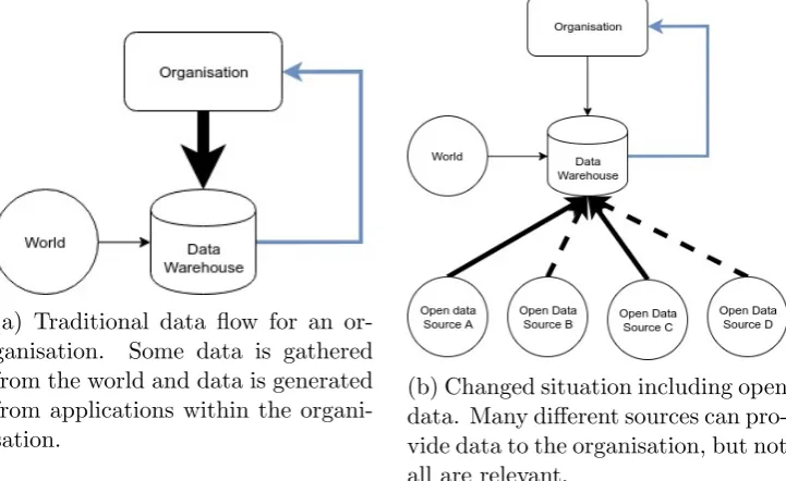
These extra data change the way that organisations can use data sources, as shown in figure 1.1. Traditionally, organisations use the data generated by themselves, in addition to some data that is gathered from the world around them (1.1a). These data are structured according to the needs of the organisation and they have influence on how this is designed. Because the amount of external data is small, the benefits of such an implementation outweigh the costs and thus effort is made to import these data into its internal data sources.

(a) Traditional data flow for an or-ganisation. Some data is gathered from the world and data is generated from applications within the organi-sation.

[image:6.595.118.479.427.648.2]

(b) Changed situation including open data. Many different sources can pro-vide data to the organisation, but not all are relevant.

Figure 1.1: Overview of changing data flows for an organisation due to the rise of open data

(7)

amount of data coming originating the organisation is relatively small com-pared to the complete set.

Organisations do not have influence on how this data is gathered, pro-cessed and published. This means that every different data source has a different way of publishing, can have a different level of trust and has dif-ferent areas of expertise. It becomes a challenge to incorporate these data, because it is expensive and time-consuming to process the data from all these different sources by hand. This challenge often means the data is not incor-porated at all, neglecting the opportunities these data can provide.

To enable effective use, several challenges need to be resolved. First of all, there are technical challenges. These include different data structures, different formats, difficult accessibility, etc. Usually, these problems can be resolved when the data is loaded into a data analysis tool and scripts can be created that load the cleaned data into the tool. This process often forms a big part of time spent by data analysts, because it can become very complex. Because this process takes place before the actual tooling is used, insight in this process is lost and the transformations (and possible errors during it) become invisible.

Another challenge concerns the context of the data. Values in themselves lack any meaning. Their meaning is defined by the context that they are put into. The number 42 in itself does not mean anything, but when it is stated that the number represents “the percentage of males”, suddenly it has meaning. This still is not a complete picture, as asking the question “The percentage of males in what?”. The context could be further enhanced by stating it represents the percentage of males within the Netherlands. There are many questions that can be asked on what the data actually represents. Then again, even when its exact meaning is known, the context is not complete. There is no information on, for example, when this measurement is taken or how it is taken (or calculated). This measurement might be taken only within a small group and not be representative. The measurement might be performed by a 4-year old, decreasing the trust in this certain measure-ment. Or someone might have calculated this number based on personal records from ten years ago.

More concretely, we state that these open data sources cannot be directly used within organisations, because:

(8)

• The context of the data (what is measured, how it is measured) is not present directly in the data itself and harder to interpret because the source is not directly from the organisation itself.

• The source may be of low quality. This includes missing values, wrong values, slightly different values that can’t be compared easily or differ-ent keys to iddiffer-entify differdiffer-ent meaning.

1.2 Project goal

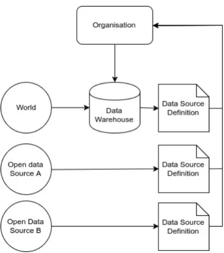
We argue that extensive use and structuring of metadata enables the use of this context during data analysis and generalise analysis methods based on these metadata structures.

Metadata are used during data analysis to provide meaning. A trivial example is data stored in a database, where the table in the database is pre-defined which defines the columns (often including types), and thus structure. This table provides the context in which data can be retrieved. Usually this use of metadata is very limited and much information about the analysis result itself is kept inside the data analysts mind.

By enriching this metadata and creating a structure for it, more extensive documentation of the context of data retrieval is possible, as well as docu-menting data results within this enriched context.

(9)

[image:9.595.180.409.123.381.2]

Figure 1.2: A schematic overview of data flows for an organisation using data source models

To be able to properly design these metamodels, we pose the following research questions.

RQ 1. What elements are necessary to create a metamodel able to represent existing datasets?

RQ 2. How can we create models for existing datasets efficiently?

RQ 3. What is the best method to define a generalized query in terms of this data model?

RQ 4. How can the generalized queries be transformed to executables able to retrieve data?

RQ 5. How can the context of the data be represented and propagated in the result?

(10)

1. is able to load open data in a raw form,

2. allows users to put these data into context,

3. eases re-use of analysis methods on datasets

4. enables analysis methods on these data that maintains this context,

5. and allows for easy publishing of results of this analysis to the end user.

1.3 Project approach

The project goals require a method to structure abstractions and properly define these, which is why we deem Model-Driven Engineering (MDE) to be a suitable approach for solving this problem. MDE allows us to explicitly define the structure of required models as meta models. Functionality is de-fined in terms of these meta models. This allows us to define functionality for all datasets that have a model defined within the constraints of the meta model.

With the use of MDE comes the definition of a transformation toolchain, consisting of metamodel definitions and transformations between them. Trans-formations are defined in terms of the metamodel, but executed on the mod-els. These transformations describe the functionality of the framework. This toolchain defines the inputs, outputs and steps required to generate the out-puts from the inout-puts.

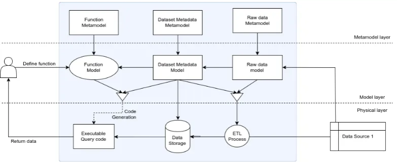
To provide an overview to the reader, the transformation toolchain used in the remainder of this report is introduced now. Figure 1.3 shows this chain. The most important models and metamodels are shown, as well as their relation between them.

The top layer represents the metamodel layer and contains metamodels for the dataset, function and raw data. The middle layer, called model layer, contains instances of these metamodels and represent actual datasets, functions and raw data sources. The bottom layer represents the physical layer. Only here is data transformed, executed and modified and upper layers only store information about the metadata.

(11)

[image:11.595.103.495.127.287.2]

Figure 1.3: A high level overview of the steps of the envisioned solution. The dataset model forms the center, functions are defined in terms of this model and a method of converting the data to this model is needed as well. The bottom layer represents the data-flow that is needed to perform the actual analysis.

This executable retrieves the results from the data as specified by the func-tion model.

We defined the metamodels for the dataset and function based on research on existing data analysis methods and metadata modeling techniques. Then, transformations based on these metamodels are defined that allows a user to transform these models into executable code. This executable code retrieves the data from the desired data source and provides the user with the desired result.

A prototype is implemented based on the definition of the metamodels and transformations and present how these cases can be solved in terms using the prototype. We focus on the metamodels that define the metadata and operations and deem model-mining of existing datasets out of scope for this project.

(12)

1.4 Structure of the report

(13)

Chapter 2 Background

Data analysis and the use of its results is already often used in businesses. They use techniques to analyse these data and use them to make better decisions. This history brought techniques to perform data analysis and strategies to apply these to policy decisions. These policy strategies are investigated in this chapter to provide a better view on the requirements of data analysis.

Similarly, solutions to perform data analysis are investigated. These in-clude storage solutions like databases, as well as libraries to directly transform data. The last element required as background is the effort others put into describing metadata of datasets.

2.1 Data-driven decision making

The huge amounts of data available today enables opportunities for analysis and extraction of knowledge from data. Using data as a foundation to build decisions upon is referred to as data-driven decision making. The goal is to analyse the data in such a way that it provides the right information for the people that need to make the actual decision. As described in the introduction, this process changes when open data is added as an additional source. To support the modeling process, this chapter explores the different opportunities for using open data within this process.

(14)

[image:14.595.219.376.175.329.2]

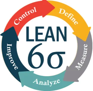
Six Sigma consists of an iterative sequence of five steps: Define, Measure, Analyze, Improve and Control, as shown in figure 2.1.

Figure 2.1: A schematic overview of the cycle of the six sigma approach

Define Based on an exploratory search through data, problems can be iden-tified or new problems can be discovered based on new insights provided by the data.

Measure When a problem has been defined, data can aid in measuring the scope and impact of the problem, indicating its importance and priority.

Analyse Analysis on relations between different problems and indicators, enabling insight on the cause of the problem or methods to solve it.

Improve Using prediction modeling, different solutions can be modeled and their impacts visualised.

Control Data can provide reporting capabilities to validate actual improve-ments .

(15)

starts again.

Open data can improve these steps by providing additional information that is traditionally outside the data collection scope of the company.

Define Open data can show additional problems that the company did not consider, because there was no insight. They can also provide informa-tion on topics that the company needs informainforma-tion for, but has not got the resources to collect these data.

Measure External sources give unbiased information and can be used to validate observations made by the organisation.

Analyse The wide scope of open data makes it possible to more extensively investigate relationships and compare different areas of interest. For example, a observation is made that sales decreased significantly. Anal-ysis shows that the market for the sector as a whole dropped, which may indicate the problem is external rather than internal and changes the view on the decision to be made.

Improve External prediction numbers can be used to either foresee future challenges, or incorporate these numbers in models from the company to improve these.

Control Use the additional information to gain extra measurements on the metrics that are important.

The additional value of open data is expected to be generally in the define, measure and analyse steps. Improve and control indications are very specific to the company itself, and therefore usually measured by the company itself. The define, measure and analyse steps are also targeted at gaining informa-tion from outside of the company, which is an area that open data holds information about. Cases in chapter 3 will show concrete examples of differ-ent business questions that can be answered within separate steps.

[20] takes another approach and divides qualitative data analysis applied policy questions into four distinct categories:

Contextual identifying the form and nature of what exists

Diagnostic examining the reasons for, or causes of, what exists

(16)

Strategic identifying new theories, policies, plans or actions

These four categories divide the different policy questions arising from the different steps from the business improvement models.

Insight on a business level is best obtained when insights are visualised well using the appropriate graph type, like a scatter plot or bar chart. These visuals directly show the numbers and give insight in the different questions asked. It is very important to choose the right type of visualisation, because this choice has impact on how easy it is to draw insight from it. This choice is based on what needs to be shown, and the type of data. [14] identifies the following types of visualisation, based on need:

Comparison How do three organisations compare to each other?

Composition What is the age composition of people within Amsterdam?

Distribution How are people within the age range of 20-30 distributed across the Netherlands?

Relationship Is there a relation between age distribution and amount of children?

The risk is that the most insightful graphs hide data to avoid clutter. While this allows the visualisation to convey meaning, it can be misleading as well. It may be not clear how much of the data is neglected, if there were any problems during aggregation, if there is missing data, how the data is collected, etc.

Important to note is that the questions for qualitative data analysis do not directly correspond to the different graph types. Policy questions are generally too complex to grasp within a single graph. [18] defines a iterative visual analytics process that shows the interaction between data visualisation, exploration and decisions made. They argue that a feedback loop is necessary, because the visualisations made provide knowledge, which in its turn can be used to enhance the visualisations made and models underlying them. This improves the decisions.

(17)

2.2 Sources for data-driven desicion making

Data is the key component for proper data-driven decision making. Organ-isations often use internal data that they collect based on the metrics they aim to analyse. These data may be too limited to be able to base conclusions on, or the use of additional sources might lead to more insights that internal data alone would be able to.

To increase the amount of data used for the decision, open data can be freely used to enable new insights. Open data are generally data published by the government and governmental organisations and are published to increase transparency within the goverment, and allow other organisations to provide additional value to society by the use of these data. The main guidelines for open data are the FAIR principles [3]:

Findable which indicates that there are metadata associated with the data to make them findable

Accessible in the sense that the data are available in a standardized, open communications protocol and that the metadata still keeps available, even if the data are not available anymore

Interoperable data uses a formal, accessible and open format and complies with the open data ecosystem.

Re-usable which ensures that data are accurate as a clear and accessible usage license.

These guidelines aim for easiest re-use of data. The vision of the gov-ernment to actively engage in publishing these data is relatively new, and publishing organizations themselves are still searching for the right approach to publish these data. This creates a diversified landscape and makes it harder to use these data. Although the publishing organisations try to ad-here to the FAIR principles, the diversified landscape and the barriers it provides leave many opportunities for the use of these data not used.

Strictly speaking, open data could be open data if it is just a plaintext file somewhere on a server. This, however, scores very low in every aspect of the FAIR guidelines. Just publishing some files is generally not enough to let people reuse the data in an efficient manner. It is important to know more about the dataset.

(18)

data or possible codes that are used. The knowledge of these elements must be published alongside the data for it to be actually useful. To facilitate an open data platform, models have been developed that model these metadata and generalise it for the users.

Other than just the meaning of data, having multiple data sources brings additional problems for the data analysis. Different formats, structures and meaning is difficult to understand. To be able to use the data, data analysts have two choices. Either they convert all needed data into a format they are comfortable with, or they use tooling that is able to use these multiple data sources.

2.3 Data analysis solutions

We investigate data analysis solutions that are widely used nowadays. These provide the foundation and inspiration for the analysis models that we pro-vide. In general, there are three distinct problems that a data analysis solu-tion needs to solve:

Data structure A definition of the data structure is needed to know how the data is stored and how to access this. This can be very simple, like an array, or very complex like a full database solution. A con-sistent structure allows standardisation of operations, while different structures may be appropriate for different data.

Data operations The analysis consists of a set of operations that are exe-cuted on the data. Because operations need to access the data, these can only be defined in terms of the structure of the data itself.

Data loading Data needs to be loaded in the desired sturcture, which is mostly not the case. To be able to load the data appropriately in the new structure, it might be neccessary to define operations that transform the data into a suitable form.

One approach is to organise all the data required into a singledata ware-house, which is a huge data storage in a specified format. In such a solution much effort is spend to define a suitable storage mechanism that stores the data for easy analysis. This approach is usually taken when questions about the data are known beforehand, because the storage solution is generally optimised for analysis, rather than the original data.

(19)

customers to allow for analytics of orders per customer, orders per time and other metrics that indicate how well the business is performing. These data originate from internal systems with underlying data storage. Sales might originate from the payments system, a complex webapplication that running a webshop, or an internal software application for customer relations.

By defining anETL pipeline, data warehouses automatically load exter-nal data into the warehouse. Just like the data storage, this ETL pipeline definition can be very complex, and is always specific for the data warehouse it is designed for. This means that the data operations used are not reusable and it is hard for users to trace the origin of the data. Reuse and interpre-tation of these data is highly dependent on the level of documeninterpre-tation that is provided.

When we step down to a lower level, we can investigate different tech-niques. We choose these techniques based on their widespread usage and different use case scenarios. The data analysis solutions we investigate are:

SQL orStructured Query Language is the best known and most used query language, and is a standardized language for querying databases. Many dialects exist for specific database implementations and their features, but all dialects share the same core. It acts on 2-dimensional data structures, referred to as tables. Usage of SQL requires the definition of these tables in the form of typed columns 1.

OLAP or Online Analytical Processing has specific operations to change cube structures. Its data structure differs compared to standard SQL in the sense that it uses multiple dimensions. Languages that allow querying over OLAP structures define operations that deal with this additional data structure.

Wrangling language, by Trifacta is a language that backs the graphical application that Trifacta makes, which lets users interact with their data to clean it. The steps the user performs are captured in a script in this specific language, which can be executed on the data.

Pandas library is a data analysis library for python that allows users to perform data operations on a loaded DataFrame, which is a 2-dimensional data structure.

All data processing libraries have their own vision on how data analy-sis should be performed ideally and differ in expressiveness, usability and

1_{although typed columns is the most used implementation, there are implementations}

(20)

method of usage. SQL and OLAP are complete data storage and query pos-sibilities and targeted to provide more data analytics, rather than extensive data science operations. The trifacta language is more extensive than SQL with regard to operations and transformations on the data and aims at pro-viding a solution to be able to interactively clean your data. The pandas library provides data analysis capabilities to python. This aims partially at solving the same problems as the trifacta language, but provides an API as first-class citizen, rather than providing a language for a user interface.

2.3.1 Database storage

Database storage is a method to storage data in a permanent manner. Be-cause they store data, they provide structure over the data they store and have methods to make this data accessible. All database solutions have methods to extract data from it.

SQL based databases are one of the oldest and stable storage solution available. Database packages like PostgreSql, MySQL or Oracle provide databases that can be queried using SQL. Queries are executed on a tables, which are defined in a database schema.

Such a schema describes a set of tables and which columns exist in which table. Based on such a schema, users can insert rows into the database, retrieve rows, and delete rows.

These databases provide 2-dimensional storage.

2.3.2 Pandas

Yet another option to define data transformations is the pandas library for python, which is often used in the data science community. Pandas works with the data structures Series, which essentially is a list of values and DataFrames which is a 2-dimensional data structure. The expressiveness of python allows users to define data operations in the form of simple equations that can quickly become more and more complex.

By the nature of being a python library, pandas makes it possible to use pre-defined functions on these data structures and by creating a very extensive set of functions it allows users to be very expressive with their data analysis. This allows users to define complex analysis methods and perform operations on the level of expressiveness that python provides, rather than the sometimes limited data operation functions in SQL.

(21)

but the user is limited to the built-in functions its specific database engine supports. Pandas allows users to define an arbitrary function based on a Series data structure and a new Series can be created that draws the value based on this function. These functions are limited to the possibilities of a python function definition, which essentially comes down to no limits.

2.3.3 OLAP

The 2-dimensional data structure of SQL has its limits, especially for ag-gregated data sources. The On-Line Analytical Processing cube, or OLAP for short is a storage and query method targeted at multi-dimensional data. This is one of the reasons this technology is mostly used in data warehouse. Just like SQL databases, OLAP databases require a pre-defined schema to be able to load the data into. But because it uses a different storage mechanism, it can provide additional operations that operate specifically on the dimensions as specified in the schema.

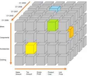
The OLAP concept has been described by different researchers and many derivatives have been defined that differ slightly in form of definition or op-erations that have been defined. We will make a simple definition based on these concepts and make an illustration of the operations that have been defined. Its goal is to define a base when OLAP is referenced elsewhere in this report.

We describe the OLAP cube on basis of figure 2.2. A single OLAP cube has multiple dimensions with distinct values. For each combination of dimen-sion values, there is a box that has a value for every metric defined. Figure 2.2 shows a cube with three dimensions, which is the largest dimension count that can be visualised easily. The cube itself, however, is not limited to three dimensions and can have many more dimensions.

While this visualisation is very simple, in practice these cubes can become very complex. Often, dimensions inherit hierarchies that aid the user in quickly collecting data. For example, there is a time hierarchy that gives an overview of sales per day. It is often desirable to view these numbers also per week, per month or per year. In OLAP cubes, these values are also calculated and stored in the cube. These data can then be queried easily, without the need for many calculations.

(22)

[image:22.595.161.451.127.382.2]

Figure 2.2: Schematic representation of an OLAP cube with three dimen-sions. Every smaller cube in the center represents a set of metrics and its values.

requires a definition that is able to capture this complexity.

We will use the definition of a direct acyclic graph. This allows for ar-bitrary parent-children relationships, while removing the complexity arising from cyclic definitions.

OLAP cubes are designed to be able to provide insight to the user inter-acting with it. Operations can be defined that allow a user to query the data within the cube, and extract the desired results. Although these operations may differ from implementation to implementation, the essential operations are:

Selection Select a subset of metrics. In the visualisation, this corresponds to taking a smaller section of each box.

(23)

sub selection of these boxes is made.

Roll-up Because the dimensions contain hierarchies, conversions between the levels of these hierarchies can be made. A roll-up is navigation to a higher level in the hierarchy. The limit is when all values for a dimension are summed up to a total value.

Drill-down Drill-down is the opposite of roll-up. It steps down a level in a dimension hierarchy. The limit of drilling down is defined by the level on which data is available.

Operations on multiple cubes are more complex, because the complexity of the dimensions needs to be taken into account. A Cartesian product, for example, creates a values for every possible combinations across the dimen-sions. This also means that metric values are duplicated across the cube and that the dimensions do not apply to every metric contained in the box. This makes the cube much harder to define and interpret.

2.4 Metadata modeling

Apart from the solutions for applying data transformations, metadata defi-nitions are an essential element as well. Metadata is data describing data. Definitions of metadata are even more broad than data itself and can consist of a wide variety of properties. While the description of data structure is the most essential for data processing, other elements are necessary to provide meaning to the data.

A proper definition to describe these metadata is hard, because there are many elements to consider. Hence we start with an identification of the elements and different use cases that users require for these metadata.

Metadata is used by users to let them understand the data it represents. Essentially, the metadata should provide answers about the data that the users can ask to their selves. Questions like: Where do these data come from? or What are the quality of these data?.

(24)

Category Definition

Definitional Convey the meaning of data: What does this data mean, from a business perspective?

Data Quality Freshness, accuracy, validity or completeness: Does this data possess sufficient quality for me to use it for a spe-cific purpose?

Navigational Navigational metadata provides data to let the user search for the right data and find relationships between the data

Lineage Lineage information tells the user about the original source of the data: Where did this data originate, and what’s been done to it?

Table 2.1: An end-user metadata taxonomy defined by [16]

Different efforts have been made to standardize these metadata [7]. DCC provides a set of metadata standards that aim to describe different methods of describing metadata. We observe that many of these specifications are based on a single domain, and describe only the meaning of the data (defi-nitional).

One of the standards described isDCAT [15], as developed by Fadi Maali and John Erickson. The goal of DCAT is to promote interoperability between different data catalogs, such that datasets can be indexed across different platforms without the need of duplicating the complete dataset. A dataset here is defined to be a file or set of files. DCAT standardizes properties that describe the file and properties of the data as a whole, like title, description, date of modification, license, etc. These attributes can be used during the implementation of a data catalog application that can then easily share its definitions with another catalog built on top of DCAT.

Because it is aimed towards data catalog interoperability, it does not pro-vide information on the data itself. Within terms of the above taxonomy: it provides information in definitional and navigational context on a high level. To some extent information about lineage, because it can be queried for the source, but it is not guaranteed that this source is the original source and does not provide information about transformations applied to the data.

(25)

provenance information in heterogeneous environments such as the Web.”. Based on the research for PROV, eight recommendations are provided to support data provenance on the web [8]. There recommendations focus on how to incorporate this provenance into a framework, like“Recommendation #1: There should be a standard wary to represent at minimum three basic provenance entities: 1. a handle (URI) to refer to an object (resource), 2. a person/entity that the object is attributed to and 3. a processing step done by a person/entity to an object to create a new object.”. Incorporating these recommendations allows for a more complete and transparent provenance framework.

While these solutions provide a standardized solution to provide metadata about the dataset as a whole, this still misses much of the context of the data itself. The data analysis solutions described above provide this information on a lower granularity to some degree, but still miss much information. SQL databases, for example, provide information the table information and some types, but lacks further description. OLAP cubes provide some additional information, but still lack much information.

Even using all these solutions does not provide much information on data quality. This quality metadata is broad, because there are many different quality issue sources that occur on different levels. On the lowest level, someone might have entered a wrong number in the database and this single value is wrong. A level higher, there could be a systematical error in a single column (e.g. leading or trailing white space), or the complete dataset could be having issues.

(26)

Chapter 3 Case Studies

To illustrate concepts, we will introduce two case studies. These cases orig-inate from a discussion group consisting of 11 board members of public or-ganisations throughout the Netherlands. This group discusses open data, use thereof inside their organisations and the impact it will have on their decision making processes. These cases thus arose from practical policy de-cisions that proved to be difficult because there was not enough insight for a substantiated choice.

This chapter indicates the insights required for policy decisions and sub-sequently gives an indication of the technical elements required to generate these insights.

3.1 Case 1: Supply and demand childcare

The first case involves supply and demand for childcare services. A large childcare services organisation with multiple locations wants to open a new location. The success of a childcare location is highly dependent on the demand close to it. Without children, there are no customers and the location set up for failure.

Before making this decision, it is essential to have an indication of the demand within possible locations. This could be done based on feeling and knowledge of the decision maker, but this relies heavily on his or her knowl-edge and is subject to biases from this person.

(27)

[image:27.595.142.454.127.275.2]

Figure 3.1: A screenshot of cbsinuwbuurt.nl, with a chloropleth map visual-isation of the amount of married people per neighborhood

Such a visualisation requires us to reduce data sources to a single value per neighborhood, which can be mapped to a color to represent that neigh-borhood on the map. This number could, for example, be calculated using a model for supply and demand, which requires us to look at supply and demand separately.

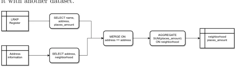
The supply is defined as the amount of places available for the childcare services. This can be estimated with good accuracy, because the register with all certified locations is published as open data. The National Registry for Childcare [4] (‘Landelijk Register Kinderopvang en Peuterspeelzalen’ in Dutch) registers every location and amount of places available per location, which directly gives a good indication of on what locations there is a lot, of little supply. The integral dataset can be downloaded as an CSV file through the data portal of the Dutch government [6].

Based on this information, one of the analysis methods that could be performed is to plot the numbers of the amount of places for each location on a map. This quickly gives a visual overview of where there are places available. Even though this requires some technical knowledge, there are many tools available online that allows a novice user to perform this operation and view the map.

(28)

[image:28.595.101.495.136.247.2]

it with another dataset.

Figure 3.2: The data flow for the data to be retrieved from the register

All in all, even this simple question results in a data processing pipeline that requires us to integrate multiple datasets. When only presented with the end result, critical policy makers immediately will ask questions like: ”How are these results calculated?”, ”What is the source?”, ”How trustworthy is the source?. This is because all assumptions made can highly influence the final results, and interpretation for these people is critical.

The resulting map gives insight on the places with high supply, but does not provide enough information. A location where few places are available might be a tempting, but is not relevant if no one lives in the neighborhood. Data indicating the supply is just as important. Since no exact numbers available, an indirect approach will be used. Various demographic properties of neighborhoods can be used to provide an indication. While this does not provide us with exact numbers, it can provide the right insights. Because this report focuses on the technical results, rather than the policy information, we will use simplified model that only uses information available already as open data. This model uses the following properties as an indicator for high demand of childcare services:

• Number of inhabitants

• % of inhabitants between 25 and 45 years

• % of people married

• % of households with children

(29)

[image:29.595.103.494.128.244.2]

Figure 3.3: The data flow for the data to be retrieved from the CBS

3.2 Case 2: Impact of company investments

The second cases concerns insights in the investments made by Oost NL. Oost NL is an investment company with the goal to stimulate employment within provinces Overijssel and Gelderland. The insight they require is twofold. On the one hand, they require insight in the impact on their investments. Since investments are not targeted for profit, but for economic growth, it is hard to measure. Insight in what investments do have an impact and what investments do not can aid them in better guiding their investments.

Another insight that they require is what companies are suitable for an investment. Generally, investments target companies and startups who inno-vate. When Oost NL wants to invest in a certain business sector, they look for companies within the regions they think it is possible to find a suitable investment. Where they look is mainly based on assumptions, which may or may not be completely off.

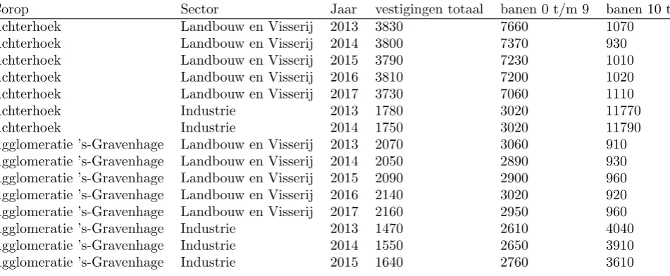
Much open data is available based on registers of companies. One of the registers in the Netherlands is LISA [5]. LISA gathers data from a national questionnaire send to companies and publishes open data based on aggrega-tions of this questionnaire. Table 3.1 shows one of the open data sets that can be generated from their site. It shows the amount of business locations in that specific region, per year and per business sector, including the amount of employees summed up in that region.

These data can be used to investigate trends of growth per sector, per region and create a baseline for growth.

(30)

[image:30.595.115.591.152.348.2]

Table 3.1: An excerpt of open data provided by the LISA register

Corop Sector Jaar vestigingen totaal banen 0 t/m 9 banen 10 t/m 99 banen>100 banen totaal

Achterhoek Landbouw en Visserij 2013 3830 7660 1070 900 9630

Achterhoek Industrie 2013 1780 3020 11770 15070 29860

Achterhoek Industrie 2014 1750 3020 11790 15030 29850

Agglomeratie ’s-Gravenhage Landbouw en Visserij 2013 2070 3060 910 420 4390

Agglomeratie ’s-Gravenhage Industrie 2013 1470 2610 4040 7850 14500

open API, and thus more easily accessible without using your own data stor-age solution.

Investments of Oost NL are often long-term and there are many factors having influence on the performance of the companies they invest in. This makes it hard to generate visualisations that undoubtedly show the impact of their investments.

From a research perspective, it is necessary to compare the growth of the companies invested in to growth of companies that did not receive this investment. One method can be to create a visualisation in which the growth of a company is compared to the growth of its sector and region, or compare its growth with similar companies throughout the Netherlands as a whole.

Measuring growth in such a manner will never become an exact science, but can provide valuable insights. These insights can best be obtained when growth is measured across as many relevant measurement scales as possible, i.e. compare it in as many relevant ways as possible. Which comparisons are relevant and which are not are to be determined by the business experts.

Oost NL uses a topsector classification for their companies, while registers (and thus resulting data) in the Netherlands usually categorize the companies using the SBI [2] (Standardized Company division). This SBI categorisation is, however, not insightful for Oost NL because this categorisation does not align with their investment portfolio and targets.

(31)

hierarchical tree structure. The root is “Total”. The second layer represents the most high level categorisation. Then, every category is categorised in smaller sub-categories.

The topsector classification Oost NL uses is a simpler subdivision across 8 different categories. These 8 categories represent the important sectors for their innovative investments, and companies that do not fall into one of these essential categories are classified as “Other”. This allows Oost NL to focus on the companies that are important for them.

To be able to use datasets with the SBI classification for comparison, we need to be able to convert this tree structure into the more simple topsector classification. Because the SBI categorisation is more explicit and contains more information, it is impossible to accurately map the sectors to this SBI code dimension.

(32)

Chapter 4 Dataset modeling

This chapter introduces the first element of the proposed solution, being a dataset metamodel. This metamodel describes the structure for a model that describes the metadata of a dataset. A DSL is generated off of this metamodel that can be used to create model files for different open data sets. Such a model then directly represents the metadata of the dataset.

4.1 Metadata

The metadata should aid users, as well as machines, to be able to read and interpret the data. While users mainly use it to understand the data, machines process the data and need to understand it in their own manner. A proper metamodel is able to fulfill these tasks for a wide variety of data.

Chapter “background” did show techniques to describe metadata. There is, however, no existing metamodel suitable for our goals, requiring the defi-nition of a custom one.

The elements required in this metamodel depend on the definition of “to understand” within the context of the data. To identify and classify what elements belong to this, we take a pragmatic, bottom-up approach, based off of questions that the metadata should be able to answer. We noted these and classified them into the following 6 categories.

Origin What is the original source? Who created or modified it? How old is it? Who modified the data? How is the data modified?

Distribution How can it be accessed? How can I filter or modify data?

(33)

Scope What region/time/values does it cover?

Structure What is the size of this dataset? What are relations between different elements?

Interpretation How should I interpret it?

More formally, to make the data understandable the metamodel should provide an abstract interface that allows processing steps to be defined and applied, independent on the data its concrete representation. Additionally, it should capture additional information about the context of the data. The combination of these two elements creates a structure allowing interaction and processing of the dataset while containing the information about its context.

4.2 Data structures

As an starting point, the two different datasets needed by case 1 will be analysed using these questions. Case 1 concerns supply and demand for childcare services and mainly uses two different data sources. The first source is the register of childcare services and the second source is the regional information from the CBS. These sources are representative of many open data sources, as we will discuss later.

The childcare service register provides an overview of every location in the Netherlands where children can be taken in. An excerpt of this dataset is shown in table 4.1. These data are published in CSV format and is structured such that every row represents a single childcare service. For each service, it provides the type of service it offers, its name, its location, amount of places and responsible municipality.

This source is representative of different registers of locations, companies, buildings or organisations that may have data that is structured in a similar format. Such a source contains a row for each instance and has columns for each of its properties.

Table 4.1: An excerpt of the register childcare services with the headers and 5 rows of values representing childcare services in Enschede

type oko actuele naam oko aantal

kindplaatsen opvanglocatie adres

opvanglocatie postcode

opvanglocatie

woonplaats cbs code verantwoordelijke gemeente VGO Hoekema 4 Etudestraat 45 7534EP Enschede 153 Enschede

(34)

The other data source for the first case originates from the CBS, and is accessible through the CBS’ OData API. In addition to providing the raw data, it has capabilities to filter the data, perform simple operations or re-trieve additional metadata. Listing 4.1 shows an excerpt of the raw data response. Because the dataset itself is too large to show in this report (62 properties), only a single metric and the two dimensions are selected.

Listing 4.1: An excerpt of how the response looks like from the OData API from the CBS

{

"odata.metadata":"http://opendata.cbs.nl/ODataApi/OData/70072ned /$metadata#Cbs.OData.WebAPI.TypedDataSet

&$select=Gehuwd_26,RegioS,Perioden",

"value":[

{ "Gehuwd_26":11895.0,"RegioS":"GM1680","Perioden":"2017JJ00" }, { "Gehuwd_26":6227.0,"RegioS":"GM0738","Perioden":"2017JJ00" }, { "Gehuwd_26":13181.0,"RegioS":"GM0358","Perioden":"2017JJ00" }, { "Gehuwd_26":11919.0,"RegioS":"GM0197","Perioden":"2017JJ00" }, { "Gehuwd_26":null,"RegioS":"GM0480","Perioden":"2017JJ00" }, { "Gehuwd_26":null,"RegioS":"GM0739","Perioden":"2017JJ00" }, { "Gehuwd_26":null,"RegioS":"GM0305","Perioden":"2017JJ00" }, { "Gehuwd_26":11967.0,"RegioS":"GM0059","Perioden":"2017JJ00" }, { "Gehuwd_26":null,"RegioS":"GM0360","Perioden":"2017JJ00" }, { "Gehuwd_26":9118.0,"RegioS":"GM0482","Perioden":"2017JJ00" }, { "Gehuwd_26":10960.0,"RegioS":"GM0613","Perioden":"2017JJ00" }, { "Gehuwd_26":null,"RegioS":"GM0483","Perioden":"2017JJ00" } ]

}

The structure between these two data sources may seem disparate, but they are actually very similar. Both are a list of grouped values. The CSV file groups the values by row, and identifies values by the header on the first row. The OData result explicitly groups these values as sets of key-value pairs. When the keys for each set are the same, these data structures are identical albeit in a different representation.

The CSV format could be easily converted to the OData result by gener-ating key-value pairs based on the column header and the value in its column. Every row then represents an entry in the set, and the value for each column forms a key-value pair within this set. The OData repsonse can be rendered to CSV by extracting the keys to headers, and placing the values in the corresponding columns.

(35)

simple. More complex structures tend to be hard to distribute and interpret further.

Because this structure is so common, we limit the supported datasets by only supporting data that can be represented as a list of sets. The implica-tion for our metamodel is that it should accurately describe the properties of each set. Structure can be generalized, with the condition that a method is need to identify the representation.

Another important aspect is the interpretation. This can be split up into interpretation of each individual key, each individual value and the set as a whole.

The key does not provide much information. The key “Gehuwd 26” in the CBS data leaves the user in the dark with its exact representation. It could be guessed that it represents the amount of married people, but this is still not enough. Questions arise such as: Which people are taken into account? How are these people counted? What does the number “26” mean within the key?

In addition to the information the key should provide, the value pro-vides information itself as well. Each value says something about its group, but not all values are equal. Isolating the column amount of places (’aan-tal kindplaatsen’) yields the values: 4,14,4,6,4. The values are a pretty se-quence, but do not convey any meaning. Isolating the names column provides the sequence: “Hoekema”, “Peuteropvang Beertje Boekeloen”, etc. These names are not valuable on their own as well, but they do provide a means to identify a single instance, and thus the topic of the group.

Combining these two sequences yields key-value pairs that match the amount of places to the name. Adding the other information from the dataset like location and type adds even more and more information about the in-stance.

(36)

We identify the columns that cannot be removed without loss of meaning to be the identifying columns, similar to a primary key in SQL databases. When the names of the childcare instances is used as the identifying column, this column cannot be removed without loss of information. These identify-ing columns play a key role in determinidentify-ing the scope of a dataset, its topics and in combining multiple datasets.

4.2.1 Dimension and metrics

The identifying columns are an essential element of the context of the dataset, and thus essential metadata. A method to fundamentally capture these prop-erties into the dataset is by classifying a column to be either a dimension or metric. Dimensions and metrics form the foundation of OLAP databases (section 2.3.3). Yet, definitions and interpretations of dimensions in datasets differ in academia. Based on the observation about columns that can or can-not be missed, we consider a data feature to be a dimension if its row value is necessary to define the context of the value of the metrics in the same row. When classifying a column to be dimension or metric, its role in identi-fying the subject of the row is the deciding factor. If the value describes a property of the subject, it is considered to be a metric, if it puts the subject into perspective or gives an indication of partitioning of a value, it is a di-mension.

Our definition provides some useful properties. First of all, the complete scope of the dataset can be identified by just inspecting the dimensions. Be-cause these dimensions describe what the data is about, their values describe the complete scope.

This dimensional information can be further enhanced. Different keys can describe different types of a dimension. One example is the use of a dimension that describes time-related information. By adding such a type to the dimension, the scope of dimension, regional and topics quickly become apparent.

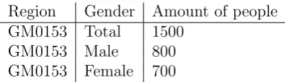
Sometimes, the structure of the data obstructs the actual use of dimen-sional information. Table 4.2 shows an example which provides information on the amount of people in a specific region (specified by a code). In this case, the region code is the subject, as all values describe a property of that region.

(37)

Region Total people Male Female

GM0153 1500 800 700

Table 4.2: An example dataset

The dataset could be just as well be represented using a single metric with “Amount of people” and two dimensions for region and gender, which would transform the dataset into the form in table 4.3. Because it now is a di-mension, it directly identifies in the metadata that information about the differences in gender is present, and that the scope is the complete set of people.

Region Gender Amount of people GM0153 Total 1500

[image:37.595.193.401.301.361.2]

GM0153 Male 800 GM0153 Female 700

Table 4.3: The example dataset in a pivoted form, using an additional di-mension

The method of converting this information is known in OLAP terminol-ogy as a pivot operation. One solution is to create an extraction process that extracts this information when importing such a dataset, but doing so would require a high level of complexity in querying and function definition. Besides that, a problem occurs when the dataset has additional metrics that are not represented in that dimension. The example shown in table 4.4 has two additional columns that are not related to the gender dimension.

Region Total people Male Female Native inhabitants Immigrants

GM0153 1500 800 700 1350 150

Table 4.4: The second example dataset

(38)

4.2.2 Aggregated vs. non-aggregated data

The difference between the two data sources is the level of aggregation. Di-mensional data structures are generally used to describe aggregated data, and the aggregation means are used as the dimensions.

For data sources that represent measurements on single entities, an spe-cific dimension type is used called “Identity”. Its values identify a single entity and requires the data source to have a feature that can be used as an identity.

4.2.3 Origin and quality

Elements important for traceability of the dataset are its origin and quality. These two properties are not essential for data analysis, and often not con-sidered in database models. But, traceability is a key element of the dataset once important decisions are based off of these data, which is part of the interpretation of the data.

The origin of the data can be split up into two categories, being the original source and the operations that have been performed on the data. These metadata should provide insight into the complete path from data aquisition to presentation of the data.

This includes information about the author, organisation that the author belongs to, method of publishing people who modified it. The credibility of the author or its organisation can have a big influence on the trustwhortyness of the data.

Another closely related metadata caterogy is the quality of the data. When data quality is higher, better conclusions can be based on these data, while low data quality can lead to skewed results.

Data quality is, like the origin, dependent on the source as well as the operations. During the data aquisition step, there is much room for error. When data originates from applications, for example, the data quality de-pends on the quality of the application. Some applications may force a user to enter data, or restrict the types of data that can be put in, which increases consistency, and thus quality, across exported datasets.

(39)

4.3 Dataset model

The above observations need to be modeled in a formal metamodel. We pro-pose the metamodel shown in figure 4.1. The root element is the “Dataset” element, which contains a key, name and description, as it is a child of the

[image:39.595.34.560.301.657.2]

Elementclass. TheElementclass is used for the most elements in the meta-model, because many elements need a key, name and description.

(40)

The dimensions and metrics form the foundation for the metamodel. The usage of dimensions allows the distinction between values that provide mean-ing to the context of the data and actual measurements. Because its usage is widespread, it allows us to build upon the results and experiences of OLAP technology for data analysis and focus on how to re-use different concepts.

The metamodel is a combination of different features provided by existing data metamodels.

• The dimension-metric model used by the CBS. We consider this model to be strong in definition of description of different properties and the grouping of metrics and dimensions.

• The dimension-metric model described by Boulil et al. [13], which is strong in defining typing and the operations that can be performed on the different types.

• The open data standard DCAT [15], which is strong in providing con-text of the dataset itself

Not all properties required for the metadata are directly described by properties in the dataset model. Table 4.5 shows an overview of which meta-data properties are covered in which manner.

Table 4.5: An analysis of the metadata categories and the level the meta-model supports

Origin The definition of author and distribution shows the source.

Distribution Definition of distribution defines the location and type of dataset. The keys of the dimensions and metrics define how these can be accessed.

Quality Validation can be done based on the units of measure-ments.

Scope This is implicitly contained in the dimensional informa-tion.

Structure The combination of dimensions and metrics shows the amount of columns and typing of different columns.

Interpretation Fine-grained descriptions allow people to specify infor-mation about the dimensions and metrics. Typing of different elements allows users to

(41)

Each column in the table needs to correspond to either a dimension or metric in the dataset model. This distinction already gives us a good indication of the meaning of the values.

Listing 4.2: The dataset model description for the dataset of childcare ser-vices

Dataset { key: lrkp

description: "Dataset met alle register kinderopvang gegevens"

dimensions: { type: identity key: id

description: "Identiteit"

}

metrics: {

type: "Measurement"

key: aantal_kindplaatsen name: "Aantal kindplaatsen"

description: "Het aantal kindplaatsen binnen deze instantie"

},{

type: "Property"

key: type_oko

description: "Het type kinderopvang"

},{

type: "Property"

key: actuele_naam_oko name: Naam

description: "Naam van de kinderopvang instantie"

},{

type: "Property"

key: opvanglocatie_postcode name: "Postal code"

description: "Postal code of the instance"

},{

type: "Property"

key: opvanglocatie_huisnummer name: "Huisnummer opvanglocatie"

description: "Huisnummer van de opvanglocatie"

},{

(42)

key: opvanglocatie_straat

description: "Straat van de opvanglocatie"

}

distributions: CSV {

url: "file:///home/lrkp.csv"

} }

For each value in the original data file, it needs to provide information on what properties these data points have, what they mean, and how we can perform operations on these sets of data points. Every row in this file is an individual data point. We can analyse this model definition based on the context definition given earlier.

The metamodel representation for the CBS dataset is given in listing 4.3.

Listing 4.3: Dataset model representation for the CBS OData dataset

Dataset {

key: wijk_kerncijfers_2017 name: "Kerncijfers per wijk"

description: "Aantal kerncijfers per wijk in Nederland"

dimensions: { type: Spatial

key: WijkenEnBuurten name: "Neighborhoods"

description: "Wijken en buurten"

attributes: {

NL00: "Nederland", GM1680: "Aa en Hunze", WK168000: "Wijk 00 Annen", BU16800000: "Annen",

BU16800009: "Verspreide huizen Annen", WK168001: "Wijk 01 Eext"

} }

metrics: {

type: "Measurement"

key: Gemeentenaam_1

description: "Testing"

}, {

type: "Measurement"

(43)

description: "Test"

}, {

type: "Measurement"

key: Mannen_6

description: "Het aantal mannen per regio gebied"

}, {

type: "Measurement"

key: Vrouwen_7

description: "Het aantal vrouwen"

}

distributions: CSV { url: "test"

} }

Due to the additional metadata the CBS provides and semantics its datasets have, modeling the results from the CBS’s OData API is more straightforward. Its aggregated data is based on dimensions and metrics, and our model implements a similar pattern for dimensions and metrics. Because the semantics already inherit dimensions and metrics, there is no design decision in what columns should be defined as dimension, and which as metric.

These groups allow us to give additional meaning to a big list of metrics for larger datasets and make it easier for an user to browse and filter these.

The dataset model provides a foundation to describe different properties of the metadata. These properties are essential to make data-driven policy decisions. Some metadata elements are not described in the dataset model. This model describes a state of the dataset. This includes structure, docu-mentation for interpretation and method of accessing. It does, however, not necessarily include complete history on the data.

(44)

Chapter 5 Function modeling

This chapter presents the DSL specifying the function that defines data op-erations, described in the form of a metamodel.

Performing operations on the data requires the definition of a function. This function enables data-analysts to specify their intentions and generate their desired results. They create a function model in terms of the function metamodel, and use the framework to transform the function to executable queries such as SQL or executable code that retrieves the results.

The definition of these functions should aid in providing information on the metadata elements stated in the previous chapter.

First, we show how the function model fits into the model driven frame-work. This should be be designed such that results can be reused, as well as direct use of results, while still maintaining a appropriate level of expressive-ness of the language.

After that, we will show its usefulness from a data oriented perspective. The metamodel needs to be constructed in such a way that the data analysis it supports is actually useful. The dataset model has already taken a step towards this goal, by using the dimension-metric model often used in data analytics.

5.1 Functions transformation structure

(45)

We opt to maintain the same levels of documentation, by structuring the documentation and operations on the data. Using a model driven solution allows us to specify the models in such a way that the documentation in-formation can be propagated. This propagation allows the data analyst to directly have documentation about the resulting data, and provide this doc-umentation alongside the dataset to inform people reusing the data.

Consider an analysis about the percentage of households with children across neighborhoods within a single municipality. Analysis is needed to determine if households with children have been declining in the city center. Such information can help case 1, regarding supply and demand for childcare services.

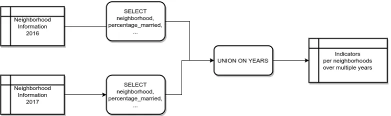
As stated, Statistics Netherlands publishes data about neighborhoods every year in a separate dataset. The information to determine a trend is available, but separation across multiple datasets encumbers retrieval in the desired format. Data from all datasets with years of interest need to be combined into a single result. This result can then be used to generate graphs and analyse it to achieve the desired result.

A possible solution is to perform an ETL process that extracts informa-tion from the separate datasets, gets the right informainforma-tion and stores its results. The result is a file or database that contains the data needed analy-sis. This works well, but insight in the process is lost and because only the data is processed, metadata about underlying sources is lost. A person using these results has no clue about the origin of the data and cannot reproduce the steps taken.

If the analyst continues working and publishes visualisations or reports based on the results, the meaning of these data is derived from the implicit knowledge the data analyst has. Errors during this process are not transpar-ent, and all implicit knowledge not documented is quickly lost after the data analyst continues with the next project.

Using the dataset model, operations can be defined that are able to mod-ify the dataset model in such a way that the desired dataset is derived. Because these dataset models represent underlying data, executing the same operations on the data generates matching results. A combination of these operations can be used to define a proper function meant for analysis.

(46)

[image:46.595.105.496.195.446.2]

level of metadata, descriptive properties and query possibilities. Automatic generation of an ETL process based off of this function definition provides the possibility to transform data and metadata accordingly.

Figure 5.1: An example of the function transformation application to a merge of the CBS neighborhoods datasets

The process of such a transformation applied to the example above is shown in figure 5.1. Two dataset models are taken and a new dataset model is created containing the information of both, accompanied by a new dimension. This new dataset model now represents the resulting data, thus the user has an overview of the meaning of the data and can share this metadata definition to help others interpret the data as well.

A model driven data analysis architecture enabling reuse and insight in open data