Large deviations and metastability in condensing stochastic particle systems

(1)

University of Warwick institutional repository: http://go.warwick.ac.uk/wrap

A Thesis Submitted for the Degree of PhD at the University of Warwick

http://go.warwick.ac.uk/wrap/45031

This thesis is made available online and is protected by original copyright.

Please scroll down to view the document itself.

(2)

M A

E

G

NS I

T A T MOLEM

U N

IV ER

SITAS WARWICEN

SIS

Large Deviations and Metastability in Condensing

Stochastic Particle Systems

by

Paul Ian Chleboun

Thesis

Submitted to the University of Warwick

for the degree of

Doctor of Philosophy

Centre for Complexity Science and Mathematics Institute

(3)

(4)

Acknowledgements

I would like to express my warmest gratitude to my supervisor, Stefan Grosskinsky, for

his continued guidance and support. It seems his door was always open, and he always

found time for very useful discussions. He has always been happy to share his knowledge

and insight, with enthusiasm and patience.

I would also like to thank all the other members of the DTC for making my time in

the department so pleasurable. In particular my second supervisor Ellak Somfai. Also

Robin Ball, for ensuring that the DTC was such a success and still finding time for very

insightful discussions. I am very grateful for the many happy discussions I have had

with colleagues in the department on this work, as well as many other things. Moreover

I would like to thank Anthony Woolcock, Peter Jones and Steven Hill for their careful

reading of this thesis.

Additional thanks go to the many people outside of the department with whom I

have had the great pleasure of discussing my work, and who responded with helpful

suggestions. I am very grateful to Michalis Loulakis and In´es Armend´ariz for pointing

out the particular local limit theorem for triangular arrays used in Chapter 3. Also

thanks to Gunter Sch¨utz, Hugo Touchette and Rosemary Harris for their support and

advice.

Finally, I would like to thank my family for their constant support. I am especially

grateful to Sarah Lloyd for her continuing support and affection, and for looking after

me so generously in the last month or so of writing-up.

This work was supported by the Engineering and Physical Sciences Research Council as

(8)

Declarations

This work has been composed by myself and has not been submitted for any other degree

or professional qualification.

• The work of Chapter 4 has largely been published in [25].

• Work from Chapter 3 and 6 will be submitted for publication.

• Chapter 5 extends results of Grosskinsky and Sch¨utz [66], and significantly

sim-plifies the analysis giving rise to the equivalence of ensembles. The analysis also

extends the stationary results to give full large deviation properties of the

maxi-mum. This gives original insight into the dynamics of the condensate. This work

(9)

(10)

Abstract

Condensation, or jamming transitions, are observed throughout the natural and so-cial sciences as prevalent emergent phenomena in complex systems, from shaken granular gases to traffic congestion. The understanding of the critical behaviour in these systems is currently a major research topic, in particular a mathematically rigorous treatment of the associated metastable dynamics. In this thesis we study these phenomena in the context of interacting particle systems. In particular we focus on two generic models for condensation, the zero-range process, and the recently introduced inclusion process.

We firstly give a brief review of some relevant aspects of Markov processes, with a par-ticular emphasis on interacting particle systems and a heuristic description of metasta-bility. Subsequently, we present a general framework for studying the equivalence of ensembles, and the large deviations of the maximum site occupation, in interacting par-ticle systems that exhibit product stationary measures. These original results are based on relative entropy methods and techniques from the theory of large deviations. They form the theoretical basis of this thesis, which enables us to find the relevant scales on which metastability is observed, and to derive refined results on the equivalence of ensembles.

The general approach is to first derive a large deviation principle for the density and maximum site occupation under a reference measure. This gives rise to the large deviations of the maximum in the thermodynamic limit, or a more refined scaling limit, which describe the metastable behaviour. Also it gives rise to equivalence of ensembles results, which are used to find the limiting expectation of important observables (such as the stationary current).

(11)

Notation

(aL) Thermodynamic scale. Scale of the large deviation principle (p. 31)

(bL) Density (mass) scale (p. 30)

¯

A Closure of the set A (p. 45)

¯

zL,m(µ) Grand canonical partition function of the restricted ensembles (p. 34)

¯ νL

m, ¯νµ,mL Restricted reference measure and restricted grand canonical measure

with restriction m. (p. 33)

B The Borelσ-algebra generated by open sets (p. 5)

Df Essential domain of the functionf (p. 31)

Eν[F] Expectation corresponding to path measurePν (p. 6)

ηx Local configuration (particle number) on site x (p. 30)

ν(f) Expectation of f with respect to measureν on the state space (p. 10)

η= (ηx)x∈ΛL Full configuration (p. 30)

1A Indicator function of the set A, 1A(x) = 1 if x∈A and 0 otherwise (p.

35)

ΛL Lattice of Lsites, connected subset ofZd (p. 30)

bxc The integer floor of a real number x∈_R(p. 23)

,() Asymptotically much smaller (greater),fngn⇔limf_gn_n = 0 (p. 45)

µ Chemical potential (p. 31)

ν=νL Reference single site marginal (p. 30)

νL Reference measure (p. 30)

ν_µL, ν_µ,mL Grand canonical measure, and restricted grand canonical measure at system size L(p. 31)

Pν Path measure of a Markov process with initial distribution ν (p. 6)

πν Measureπ is absolutely continuous with respect toν (p. 152)

π_ρL, πL_ρ,m Canonical and restricted canonical measures at system size L(p. 35)

(12)

R+ Non-negative reals [0,∞) (p. 21)

scan Canonical entropy density (p. 39)

scond Condensed entropy density contribution (p. 41)

sgcan Grand canonical entropy density (p. 40)

|X| Cardinality of the setX (p. 30)

k · k_{T .V.} The total variation norm (p. 153)

∧,∨ a∧b= min{a, b}and a∨b= max{a, b} (p. 43)

π

−→ Convergence in probability w.r.t. probability measureπ. (p. 23)

Zd d-dimensional integer lattice (p. 5)

A◦ Interior of the setA (p. 45)

Ac Complement of the setA (p. 45)

Cb Bounded continuous functions (p. 152)

C₀b Set of bounded cylinder functions (p. 37)

D[0,∞) Canonical path space of a Markov process (p. 6)

E Local state space (p. 30)

f(h) =o(h) f(h)/h→0 ash→0 (p. 6)

f∗ The Legendre-Fenchel transform off (p. 157)

fn=O(n) |fn| ≤C|n|for someC >0 andn sufficiently large (p. 45)

fn∼gn Asymptotically proportionalfn=Cgn+o(1) (p. 61)

fn'gn Asymptotically equivalent fn=gn+o(1) (p. 61)

I(ρ, m) Rate function for the joint density and maximum under the reference measure (p. 50)

Iρ(m) Rate function for the maximum under the canonical measures (p. 51)

ML Random variable onXL giving the macroscopic maximum site

occupa-tion on scale (bL) (p. 33)

P_ρL←→aL QL_µ MeasuresP_ρL and QL_µ are equivalent, Definition 3.11 (p. 36)

SL Empirical density or rescaled density (p. 30)

x, y Lattice sites (p. 30)

XL, XρLL State space XL = N

ΛL _{and canonical state space} _XL

ρL = {η ∈ XL |

(13)

(14)

Chapter 1

Introduction

Statistical mechanics is fundamentally concerned with understanding the macroscopic

behaviour of systems composed of many interacting microscopic components. Such

systems are ubiquitous in nature, from states of matter comprising a huge number of particles (of the order∼1023), through to granular media, traffic flow and crowd

dynam-ics. In principle the microscopic dynamics often follow deterministic, albeit potentially

complicated, equations of motion. However, typically it is not feasible or desirable to have a complete description of such systems on the level of the microscopic dynamics.

We therefore approximate the system in terms of an effective probabilistic description.

The origin of the apparent random fluctuations is often related to sensitive dependence on initial conditions and mixing properties of the microscopic dynamics. In practice

a mathematically rigorous justification of this approximation is often very challenging.

In many cases we cannot hope to accurately predict the microscopic dynamics, due to their complexity, such as predicting the behaviour of people in traffic flow. Due to the

large number of individual components, however, it is often sufficient to approximate the microscopic behaviour in terms of postulated probability distributions, since the

behaviour of the system on the macroscopic scale is robust with respect to the actually

origin of the noise.

The probabilistic description gives rise to a characterization of the system in terms of the expected value of certain observables. Mathematically these correspond to

mea-surable functions on the microscopic state space. It turns out that after some suitable equilibration time, in the large system size limit these observables are typically

deter-mined by a small number of macroscopic system parameters, such as the temperature

or total density. Of particular interest is the dependence of certain observables on these parameters. Phase transitions occur when the system undergoes a qualitative change in

the macroscopic behaviour as some parameter is varied. These are signalled by

singu-larities in some thermodynamic functions and abrupt transitions of some macroscopic observables.

There is a very well developed general understanding of systems of many

identi-cal components which are in equilibrium with their surroundings. Such systems are described by a Hamiltonian, or energy function, and the dynamics are assumed to be

(15)

in the long time and large system limit, the typical value of macroscopic observables are

given by the expected values under the relevant stationary measure. Such systems have

been extensively studied in the physical literature, since the seminal work of Boltzmann, and there is now a well developed mathematical theory [76, 111]. There is also a well

developed mathematical understanding of phase transitions in such systems in terms of

Gibbs measures [55].

There are two ways that the equilibrium scenario can breakdown. The system could be driven out of equilibrium, so that time reversibility is not satisfied, such as attaching a

thermal system to two heat baths at different temperatures, or similarly, if we consider

traffic on a uni-directional road. Secondly, dynamic aspects of the systems may be relevant on long time scales comparable with the typical observation times, such as

slow relaxation times from certain initial conditions. In this case, a description of the

system in terms of the long time stationary distributions for the process is no longer satisfactory. In both of these cases it is no longer clear that the equilibrium approach is

still valid, and there currently exists no such general formalism. However, such systems are ubiquitous in nature, and of significant practical importance. The models discussed

in this thesis will typically be non-equilibrium in the sense of at least one of these ways.

Frequently, we consider the case of both non-reversibility and the existence of dynamics relevant on macroscopic time scales.

A system is said to exhibit metastability if given certain initial conditions it quickly

relaxes to some apparently stable equilibrium, but on a much longer time scale a random

fluctuation or external perturbation causes it to relax to a more stable state. The characterising feature is the existence of two or more well separated time scales. This

phenomena is typically present at first order phase transitions. Metastability is well

understood on a heuristic level, however a mathematical description is an active area of research in probability theory and statistical physics [17, 107].

To clarify ideas somewhat we describe the feature discussed above in more detail for

the example of traffic modelling. We consider a single stretch of road, with two open boundaries, cars may enter at one end and move towards the exit. Any stochastic model

of traffic on a uni-directional road (such as a motorway) clearly cannot be time reversible

with respect to any stationary distribution since the system supports a non-zero current. As the total density of cars increases the flux initially increases until, at some critical

density, a jam may form and the average flux then begins to decrease. A defining feature

of such traffic models is that close to the jamming transition the system switches between metastable fluid and jammed states. Also the typical number of cars (single components)

in traffic jams is typically only of order ∼103−104. This is far fewer than the number

of individual microscopic components in classical applications of statistical mechanics, which is of order∼1023. Therefore, finite size effects are also significant in understanding

the observed behaviour in applications. Each of these issues are addressed, for a system

that can be applied as a simple model of traffic flow, in Chapter 4.

Although there is, as yet, fewer general principles that apply to non-equilibrium

(16)

[85, 94, 95]. These consist of particles that randomly jump on a lattice and whose

dynamics are influenced by interactions with each other. Formally they are defined in

terms of continuous time Markov process on a discrete state space (see Chapter 2). The specific dynamics can be chosen to represent the microscopic behaviour of some physical

system of interest. These models have been widely applied in physics, biology and social

sciences. The underlying process may naturally be defined in terms of discrete particles on some lattice, for example a system of coupled service queues, otherwise continuous

degrees of freedom may be described by a coarse graining procedure, for example when

modelling traffic. As usual we expect the phenomenology described by the models to be independent of certain details of the underlying microscopic system of interest. In this

sense interacting particle systems can be interpreted as mesoscopic models that serve as

an approximation of the true underlying microscopic dynamics. They continue to be of interest in the physics and mathematical literature due to their broad applications and

the variety of non-trivial behaviour they can exhibit, such as phase transitions in only

one dimension, whilst (in many cases) remaining reasonably tractable.

A particular interacting particle system, known as the zero-range process (introduced

in [115]), serves as a generic model for condensation and jamming transitions and has

various applications (see [42, 43, 113] and references there in). There is, a priori, no bound on the number of particles that can occupy each lattice site, and particles interact

only with other particles on the same site (a zero-range of interaction). This process has received considerable research attention recently due to its non-trivial critical behaviour.

This process, and the condensation transition, are the focus of Chapters 4 and 5. A

description of the leading order finite size effects for a generic class of condensing zero-range processes is contained in Chapter 4.

A real space condensation transition analogous to that in the zero-range process has

been observed experimentally in granular media [123]. In these experiments it has been found that the effective jump rates of particles can depend non trivially on the total

system size [117]. In Chapter 5 we study a toy model in which size-dependent jump

rates lead to an effective long range interaction, this stabilises metastability and non-equivalence of ensembles in the thermodynamic limit. Studying the thermodynamic

limit in this model can therefore help to understand the behaviour of finite systems.

This behaviour is analogous to the case of Kac potentials in equilibrium systems [107].

In the models we consider, the total number of particles (or total mass) is conserved

by the dynamics. So, restricted to finite initial conditions the processes typically exhibit

unique stationary measures. These stationary measures, called the canonical measures, describe the typical long time behaviour of the system. Calculating the expected value

of relevant observables under these measures is often not practical. A much simpler description is often found by instead fixing only the mean of the conserved quantity, this

gives rise to the grand canonical measures. One then hopes that in the limit of large

system sizes these two descriptions give rise to the same predictions for all relevant observables. In this case the grand canonical measures give a sufficient description

(17)

to phases transitions [1, 55]. Although the systems we look at are non-equilibrium

the stationary measures are essentially still Gibbs measures and many results from

equilibrium statistical mechanics still hold [54].

In this thesis we develop a general approach, based on entropy and large deviation

methods, for studying the stationary properties of a class of interacting particle systems

that exhibit condensation transitions. These results belong to a wide class of large deviation and entropy methods in statistical mechanics [1, 40, 118]. We generalise recent

methods such as relative entropy techniques, making use of refined local limit theorems.

With regards to the equivalence of ensembles our results are closely related to the work of Lewis et al. [93]. However, the results here generalise to non-compact local state

space and point-wise estimates of large deviation probabilities, which are relevant in the

systems we study. The general framework we derive allows us to consider various scaling limits, and identify the relevant scale on which metastability is observed.

Broadly, the general approach is to derive a large deviation principle for the joint

density (corresponding to the conserved quantity) and maximum site occupation under a fixed grand canonical measure [34]. This then gives rise to a large deviation principle

for the density alone, which in turn gives rise to results on equivalence of ensembles,

useful for calculating the expected value of certain observables. Also we are able to extract the canonical large deviations of the maximum site occupation, which give rise

to an effective free energy landscape for the (scaled) maximum site occupation. The

maximum site occupation turns out to be the relevant order parameter for describing metastability in the condensing systems we consider and we associate local minimum in

the free energy landscape with metastable states. Phase transitions are observed when the nature of the global minimum changes. These results could be significant for a first

rigorous analysis of metastability in such systems, as the system size diverges.

In Chapter 2 we define the models that are used in the thesis and summarise relevant results from existing literature on interacting particle systems and metastability. We

outline our general approach to studying equivalence of ensembles and metastability,

and summarise relevant technical results in Chapter 3. On first reading, the results of Section 3.4 may be omitted and used as a reference in later chapters. In Chapter

4 we apply these techniques to derive original results on the finite-size effects in a

generic class of condensing zero-range processes, which give rise to metastability in the appropriate scaling limit. In Chapter 5 we study a system for which these effects are

stabilised in the thermodynamic limit. Here we extend recent results on the stationary

properties of the system, and gain further insight into the metastability and relocation dynamics of the condensate. The general framework of Chapter 3 also gives rise to

a simpler analysis of this system than in previous studies [70]. Finally in Chapter 6,

we discuss condensation in a different model, the recently introduced inclusion process [57, 69], where condensation in the canonical ensemble has not been studied before. We

observe two distinct regimes which are dependent on an external parameter (namely the

(18)

Chapter 2

Interacting particle systems

In this chapter we give a precise definition of the stochastic particle systems that are studied in this thesis, and summarise some relevant previous results related to these

models. We introduce key concepts that will be treated throughout the thesis, such as equivalence of ensembles, condensation and metastability.

2.1 Definitions

In this section we give a precise description of stochastic particle systems largely follow-ing [95] and [86]. Relevant results for continuous time Markov chains can also be found

in [106].

2.1.1 Dynamics: Generators and master equations

Interacting particle systems are a class of continuous-time Markov processes on discrete state spaces. States in the state space define particle configurations. The dynamics are

usually specified by giving the infinitesimal rates at which transitions between states

occur.

The state spaceX of the process is the set of all possible particle configurations.

For interacting particle systems the state space is given by X = EΛ (formally given by the set of functions from Λ to E), where E is the (countable) local state space

and Λ is a countable lattice. Throughout this thesis the lattice Λ is typically a finite

connected subset ofZd, for example in the one dimensional case ΛL={1,2, . . . , L}. We

restrict our attention to processes on the one dimensional, countable local state spaces

E = N = {0,1,2, . . .}. We note that since the local state space E is not compact, X

is itself not compact. We denote configurations of X by bold Greek letters, so that for eachx∈Λ,ηxstands for the number of particles at lattice sitexin the full configuration

η = (ηx)x∈Λ ∈ X. The state space X is endowed with the product topology which is

metrizable, with measurable structure given by the Borel σ-algebra,B.

(19)

path space,

D[0,∞) ={η(·) : [0,∞)→X|η(·) is right continuous and has left limits} .

The occupation of site x at time t is given by ηx(t). Let F be the smallest σ-algebra

on D[0,∞) relative to which all the functions η(·) 7→ η(s) for s ≥ 0 are measurable.

For t ∈ [0,∞), let Ft be the smallest σ-algebra on D[0,∞) relative to which all the

mappingsη(·)7→η(s) for 0≤s≤t are measurable. The filtered space (D[0,∞),F,Ft)

serves as a generic choice for the probability space of the process.

Definition 2.1. A Markov Process on X is a collection {Pη,η ∈ X} of probability measures onD[0,∞) indexed by initial configuration inXwith the following properties,

(a) Pη[ζ(·)∈D[0,∞) :ζ(0) =η] = 1 for allη∈X.

(b) Pη[ζ(s+·)∈A| Fs] =Pζ(s)[A] a.s. for everyη∈X andA∈ F. (Markov property)

(c) The mappingη7→_Pη_{[A] is measurable for every} _A_{∈ F}_.

Property (a) states thatPη is normalised on paths with initial conditionη. Property

(b) is the Markov property and ensures that the probability of some future event

occur-ring, conditioned on the history up to some time s, depends only on the configuration at time s(memoryless). Property (c) allows us to consider the process with arbitrary

initial distributionν on X, defined by,

Pν =

Z

X

Pη ν(dη) . (2.1)

For a Markov Process the expectation corresponding toPη will be denoted by Eη,

Eη[F] =

Z

D[0,∞)

F dPη , (2.2)

for any measurable functionF onD[0,∞) which is integrable with respect toPη.

The dynamics are characterised by transition rates c(η,η0) ≥ 0 which, for all

η,η0 ∈ X, describe the rate at which the system changes from the current state η to

the new state η0. The intuitive meaning of the transition rates cis given by

Pη[η(δt) =η0] =c(η,η0)δt+o(δt) as δt&0 forη0 6=η . (2.3)

So given the state is currently η then in a small time δt the probability of the system

transitioning to stateη0 is approximately c(η,η0)δt.

Throughout this thesis we focus on systems in which the number of particles is locally

conserved, so-called driven diffusive systems (or lattice gases), in which particles move on

the lattice without being created or annihilated. For compact local state spaces there is a general theory on how to construct interacting particle systems even on infinite lattices

(20)

local state spaces which we consider in this thesis, constructions on infinite lattices can

be done on a case by case basis and require more restrictive assumptions on possible test

functions and jump rates, see for example [2] for a construction of zero-range processes. To extend this construction to inclusion processes with bilinear growth of jump rates is

an interesting theoretical problem which has not been studied so far. We do not discuss

such constructions here, since do not study processes on infinite lattices, but only scaling limits of large finite systems and their properties. On finite lattices or graphs the state

space of our models is still non-compact but countable, and therefore we are effectively

working with Markov chains and their construction is standard [95, 106].

Markov chains are well defined for all time if the process does not explode for each

initial configuration (see e.g. Chapter 2 of [106]). This is trivially fulfilled in our case

since the processes we consider conserve the total number of particles. Under every (reasonable) initial distribution we haveν[ηx <∞] = 1, so the total number of particles

on a finite lattice is P

x∈Ληx <∞ almost surely. Therefore, for every initial condition

the time evolution of the process concentrates on a finite subset of the total state space characterized by the number of particles, and explosion is impossible.

Although we only consider Markov chains, we stick to the customary formulation

using semigroups and generators in this thesis, and explain the connection to the master equation and other concepts for Markov chains in the following. Our state space X is a

countable (not necessarily compact) metric space and we denote,

Cb ={f :X→R|f is continuous and bounded} ,

regarded as a Banach space with respect to the uniform norm kfk∞ = supη∈X|f(η)|.

Functions in Cb are regarded as observables, and we define the dynamics firstly with respect to the time evolution of the expected value of all observables. In particular

cases it is possible to consider a larger class of functions, however Cb is sufficient to

uniquely characterize the distribution of the Markov chain as a consequence of the Riesz representation theorem (for example see [110], Theorem 2.14).

Definition 2.2. For a given process{Pη,η∈X}, for eacht≥0 we define the operator,

S(t) :Cb →Cb by (S(t)f) (η) =Eηf η(t) . (2.4)

In general f ∈Cb need not implyS(t)f ∈Cb, however all the processes we consider do have this property and are known as Feller Processes.

These operators form a Markov semigroup in the following sense.

Definition 2.3. A Markov semigroup is a collection of linear operators{S(t), t≥0}on

Cb with the following properties:

(a) S(0) = 1, the identity operator onCb.

(b) The mapping t7→S(t)f is right continuous for everyf ∈Cb_.

(21)

(d) S(t)1 = 1 for all t≥0.

(e) S(t)f ≥0 for all non-negative f ∈Cb_.

The importance of Markov semigroups lies in the fact that there is a one-to-one

correspondence with Markov processes.

Theorem 2.1. Suppose {_Pη_,_η _∈ _X_} _{is a Feller Markov process on} _X_{, then} _S(t) _in

Definition 2.2 is a Markov semigroup.

Also the following converse of this theorem holds.

Theorem 2.2. Suppose {S(t), t≥0} is a Markov semigroup on Cb. Then there exists

a unique Feller Markov process {_Pη_,_η_∈_X_} _{such that (2.4) holds for all} _t_≥₀_.

Proof. For proofs of these two theorems see for example [95] and [106].

The semigroup defined above describes the time evolution of expected values of

observablesf ∈Cb for a given Markov process. It provides a full representation of the

Markov process, dual to the path measures{Pη,η ∈X}. Following (2.1) and (2.2) the expectation of observables at t≥0 with respect to initial distribution ν is given by,

Eνf η(t)=

Z

X

(S(t)f)(ζ)ν[dζ] =

Z

X

S(t)f dν for all f ∈Cb .

We expect, from property (c) of the definition of the semigroup operator S(t), that it is of an exponential form generated by the ‘time derivative’ ofS at zero, S0(0),

“S(t) =etS0(0) =I+S0(0)t+o(t)”.

This is made precise in the following.

Definition 2.4. The (infinitesimal) generatorL:Cb →Cb for the process{S(t), t≥0}

is given by,

Lf = lim

δt&0

S(δt)f−f

δt for f ∈C

b _. _(2.5)

Theorem 2.3. There is a one-to-one correspondence between Markov generators and

semigroups onCb, given by

S(t)f = lim

n→∞

I− t

nL

−n

f for f ∈Cb, t≥0 .

Forf ∈Cb alsoS(t)f ∈Cb for allt≥0 and,

d

dtS(t)f =S(t)Lf =LS(t)f , (2.6)

called the forward and backward equation, respectively. Formally we write S(t) =etL

(22)

With jump rates c(η,η0) the generator can be computed directly from (2.3), for

small δt&0,

S(δt)f(η) =Eηf η(δt)=

X

η0_∈_X

f(η0)Pη[η(δt) =η0]

= X

η0₆₌_η

c(η,η0)f(η0)δt+f(η)



1− X

η0₆₌_η

c(η,η0)δt



+o(δt) . (2.7)

With the definition 2.4 of the generator, above, this implies,

Lf(η) = X

η0_∈_X

c(η,η0) f(η0)−f(η)

.

where we use the convention thatc(η,η) = 0 for allη∈X.

The description above, for Markov chains, is equivalent to a description in terms of

themaster equation as follows. The indicator functions1η :X→ {0,1}defined by,

1η(ζ) = 





1 ifζ =η

0 otherwise,

are bounded and form a basis of Cb. We denote the probability distribution on X at timet starting from initial distributionν by,

pt[η] = Z

X

S(t)1η dν . (2.8)

Since we have countable state space, we can identify measures on X with their

proba-bility mass functions and use the same symbol to avoid overloading the notation. Sub-stituting into the forwards equation from Theorem 2.3, for all η∈X,

d

dtpt[η] =

Z

X

S(t)L1_η dν= X

ζ∈X

pt[ζ] X

ζ0∈X

c(ζ,ζ0) 1η(ζ0)−1η(ζ)

= X

ζ∈X

pt[ζ]c(ζ,η)−pt[η] X

ζ0∈X

c(η,ζ0).

This gives rise to the master equation,

d

dtpt[η] =

X

ζ∈X

pt[ζ]c(ζ,η)−pt[η]c(η,ζ)

(2.9)

with intuitive gain and loss terms on the right-hand side. For Markov chains this is equivalent to the forward equation (2.6), since the indicator functions form a basis of

(23)

2.1.2 Stationary measures

A stationary distribution for the process is a probability distribution which is invariant

under the dynamics.

Definition 2.5. A measure ν on X is stationary if

ν(S(t)f) =ν(f) for allf ∈Cb .

Throughout the thesis we use the notationν(f) =R

Xf dν for the expected value with

respect to measures on the state space.

Ifν is a stationary measure then,

Pν[η(·)∈A] =Pν[η(t+·)∈A] for all t≥0, A∈ F .

Equivalently, using the master equation notation (2.8), if ν is stationary and p0 = ν,

thenpt=ν for all t≥0.

Proposition 2.4. A measure ν onX is stationary if and only if,

ν(Lf) = 0 for all f ∈Cb .

Proof. See for example Liggett [95] Proposition 2.13.

Since the indicator functions used to construct the master equation form a basis of Cb

this can be stated equivalently in terms of the master equation as;ν is stationary if and only if it solves the system of differential equations,

d

dtν[η] =

X

ζ∈X

ν[ζ]c(ζ,η)−ν[η]c(η,ζ)

= 0 for all η∈X .

Definition 2.6. A Markov process with semigroup{S(t), t≥0}isergodicif there exists

a unique stationary distribution π and,

lim

t→∞pt=π for all initial distributions p0 ,

wherept is the distribution at timet, as given by (2.8).

Not every Markov chain has a stationary distribution. However, existence of at least

one stationary distribution is guaranteed if the state spaceX is finite.

Definition 2.7. A Markov process{_Pη_:_η_∈_X_}_{is called}_irreducible_{, if for all}_η_,_η0 _∈_X,

Pη[η(t) =η0]>0 for somet≥0 .

An irreducible Markov process can sample the entire state space, from any initial

(24)

Sec-tion 3.5). The processes we focus on in this thesis are typically ergodic when restricted

to a fixed finite number of particles on a finite lattice, due to the following theorem.

Theorem 2.5. An irreducible Markov process with finite state spaceX is ergodic.

Proof. The proof is a direct result of the Perron-Frobenius theorem ([64] Theorem 6.6.1).

The generator of the process for finite state space is a real matrix c(η,η0), which has

unique eigenvalue 0, and the corresponding unique eigenvector corresponds to the unique stationary distribution.

2.1.3 Reversibility

Definition 2.8. A measureν is called reversible for the process with semigroup

{S(t) :t≥0}if,

ν(f S(t)g) =ν(gS(t)f) for all f, g∈Cb .

For Feller processes the definition is equivalent to,

ν(fLg) =ν(gLf) for all f, g∈Cb .

Choosing g = 1 in the definition of reversible we see that every reversible measure is

stationary. Under the stationary distribution the process can be extended to negative times on the path space D(−∞,∞). If the measure ν is reversible then the forward

process, with initial condition ν, has the same joint distributions as the time reversed

process.

By inserting indicator functions into the definition 2.8 we arrive at the following

characterisation on countable state spaces.

Proposition 2.6. A measure ν on countable state space X is reversible for the process

with transition rates c(·,·) if and only if it fulfils the detailed balance conditions

ν[η]c(η,ζ) =ν[ζ]c(ζ,η) for allη,ζ ∈X .

2.2 Models

2.2.1 Zero-range process

The zero-range process (ZRP) is a stochastic particle system with no restriction on the

number of particles per site and with jump rates that depend only on the occupation of the departure site. The process was originally introduced by Spitzer [115]. The simple

zero-range interaction leads to a product structure of the stationary distributions [2, 115]. These processes have been a focus of recent research interest since they can exhibit a

condensation transition (described in Section 2.3.2). Findings for the zero-range process

can be applied to understand condensation phenomena in a variety of nonequilibrium systems (see [43] and references therein), as well as providing a generic model of domain

(25)

exclusion systems [81] (see Section 2.2.2 for more details). The process continues to be

of interest; recent work on variations of the model includes mechanisms leading to more

than one condensate [84, 114, 116], or the effects of memory in the dynamics [74].

Definition

There is a-priori no restriction on the number of particles on each site, in this sense

the zero-range process is a bosonic lattice gas. The local state space will therefore be

N={0,1, . . .}. We focus on finite translation invariant lattices with periodic boundary conditions. Denote by Tn = Z/nZ = {1,2, . . . , n} the one dimensional integer torus.

We consider the zero-range process defined on the d dimensional torus, ΛL = (Tn)d,

of L = (nd_{) sites. For example in the one dimensional case Λ}

L = {1,2, . . . , L} with

periodic boundary conditions. The state of the system is described by η = (ηx)x∈ΛL

belonging to the state space of all particle configurations

XL={η= (ηx)x∈ΛL :ηx ∈N}=N ΛL _.

Particles jump on the lattice at a rate that depends only on the occupation number of the

departure site (zero-range). A particle jumps off sitex∈ΛLafter an exponential waiting

time with rateg(ηx) and moves to a target siteyaccording to the probability distribution

p(x, y). We restrict our analysis to the case of homogeneous jump distributions,

p(x, y) =q(y−x) for all x, y∈ΛL .

Further, we assume thatq(0) = 0, q is normalised, and is of finite range,

X

y∈ΛL

q(y) = 1 and q(z) = 0 if|z|> R for someR >0 ,

where R is independent of the system size L. Also p is irreducible on ΛL so that

every particle can reach any site with positive probability. The transition rates, from

configurationη to configurationζ, are given by,

c(η,ζ) =







g(ηx)q(y−x) ifζ =ηx→y

0 otherwise,

(2.10)

where ηxz→y =ηz−δ(z, x) +δ(z, y) andδ is the Kronecker delta. We assume that the

jump rates are strictly positive on the positive integers and have bounded variation,

sup

k∈N

|g(k+ 1)−g(k)|<∞ and g(k) = 0 ⇐⇒ k= 0. (2.11)

The infinitesimal generator of the process acting on suitable functionsf is given by

(L_Lf)(η) = X

x,y∈ΛL

(26)

for f ∈ Cb_(X

L) [2, 96]. In general the jump rates may also depend on the size of

the system (see Chapter 5), in this case we explicitly included the size dependence by

including a subscriptL,gL(ηx). This defines the Markov process on the countable state

space XL as described in the previous section. The process can also be defined on an

infinite lattice under certain constraints, for details see [2, 75].

For example, if g(k) = k for all k then the zero-range process reduces to the su-perposition of independent random walkers on ΛL. If g(k) = 1 for all k > 0 then the

zero-range process reduces to a system of Lqueues with mean-one exponential random

times of service.

Stationary Measures

The following summarises well known results on stationary measures of the zero-range process, for details see [2, 42, 115]. The zero-range process with generator (2.12), on a

periodic lattice, has a family of stationary homogeneous product measures onXLwhich

we refer to as the grand canonical ensemble. These measures are parametrized by a chemical potential µ∈_Rand are of the form,

ν_µL[η] = Y

x∈ΛL

νµ[ηx] where νµ[n] =

1

z(µ)w(n)e

nµ_. _(2.13)

These exist for all µ∈ [0, µc) where µc is the logarithmic radius of convergence of the

(single site) partition function

z(µ) =

∞ X

k=0

w(k)eµk. (2.14)

The stationary weights w are given byw(0) = 1 and

w(n) =

n Y

k=1

g(k)−1, n >0. (2.15)

Throughout the thesis the expect value of a functionf with respect to a measureν is denoted by ν(f) with round brackets. The grand canonical expected particle density

is a function of µand is given by

R(µ) :=νµ(η1) = ∞ X

k=0

kνµ[k] =∂µlogz(µ) , (2.16)

which is strictly increasing and limµ→−∞R(µ) = 0. The critical density is defined by

ρc= lim µ%µc

R(µ)∈(0,∞], and condensation occurs ifρc<∞, as described in Section 2.3.

It follows from the form of the stationary weights (2.15) that the expected rate of

(27)

of the chemical potential,

νµ(g(ηx)) = ∞ X

k=0

g(k)νµ[k] =eµ .

The expected jump rate off a site is proportional to the average stationary current, or, in the case that the first moment P

zz q(z) vanishes, to the diffusivity. Therefore for

simplicity, in the rest of this thesis, current will refer to the average jump rate off a

site, which is clearly site independent under a homogeneous stationary distribution. In the grand canonical ensemble the current is therefore simply given by

jgc(µ) =νµ(g(ηx)) =eµ . (2.17)

The zero-range process is reversible if and only if the dynamics are symmetric q(z) = q(−z).

The process conserves the total number of particles in the system, so XL can be

partitioned into invariant subsets,

XL,N ={η∈ΩL| X

x∈ΛL

ηx =N}, (2.18)

on which the zero-range process is a finite state irreducible Markov process. So for fixed

system sizeLand total number of particlesN the process restricted toXL,N is ergodic,

the corresponding unique stationary measures belong to thecanonical ensembleand are given by

πL_N[η] :=νµ[η| X

x∈ΛL

ηx=N]. (2.19)

These measures are independent ofµand are given explicitly by

π_NL[η] = 1 Z(L, N)

Y

x∈ΛL

w(ηx)δ X

x∈Λ

ηx−N

,

where the canonical partition function is the finite sum

Z(L, N) = X

η∈XL,N Y

x∈ΛL

w(ηx) . (2.20)

In the canonical ensemble the form of the stationary weights, Eq. (2.15), implies

that the average current is given by a ratio of partition functions,

j_Lcan(N/L) :=π_NL(g(ηx)) =

Z(L, N−1)

(28)

The canonical partition functions can be calculated iteratively,

Z(L, N) =

N X

k=0

w(k)Z(L−1, N −k) . (2.22)

Similarly we can calculate the canonical distribution of the maximum site occupation. To this end we define the cut-off canonical partition function which counts configurations

for which the maximum site occupation is less than or equal to M,

Q(L, N, M) =

min{M,N} X

k=0

w(k)Q(L−1, N −k, M) . (2.23)

This gives rise to the cumulative distribution for the maximum under the canonical measures, and allows us to calculate

π_NL

max

x∈ΛL

ηx=M

= Q(L, N, M)−Q(L, N, M−1)

Z(L, N) . (2.24)

For more details see Appendix D.1.

2.2.2 Mapping to the exclusion process

The one dimensional zero-range process, on translation invariant lattices with

nearest-neighbour jumps, can be mapped onto a simple exclusion process (a model in which each

site can contain at most one particle). From the point of view of a tagged particle in the exclusion process the systems are equivalent. This was first noticed in [50, 85], and has

been applied to the study of jamming transitions in simple traffic models [22, 53, 83].

In the simple exclusion process the local state space is E = {0,1} where ηx = 1

is interpreted as the presence of a particle at site x ∈ Λ, and ηx = 0 an empty site.

Particles are allowed to jump to neighbouring sites on the lattice only if the target site

is empty. We consider a generalised version of the exclusion process originally introduced in [115], where the rate that particles jump on the lattices is allowed to depend on the

entire configuration (we restrict our attention again to finite lattices). The generator of

the process is given by,

Lf(η) =X

x∈Λ

px(η)ηx(1−ηx+1) +qx+1(η)ηx+1(1−ηx)

f(ηx↔y)−f(η)

.

where,

ηx_z↔y =



   

   

ηy ifz=x

ηx ifz=y

ηz otherwise,

px(η)>0, is the rate at which a particle at site xjumps to sitex+ 1, given the current

(29)

[image:29.595.162.413.74.193.2]

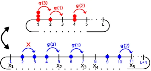
Figure 2.1: Equivalence between a totally asymmetric zero-range process and an ex-clusion process. The zero-range process is shown at the top, and the corresponding exclusion dynamics are shown below. The position of holes xi in the exclusion process

corresponds to the lattice sites in the zero-range process as explained in the text.

case most relevant for applications is that of totally asymmetric dynamics on a ring, for

which qx(η) = 0 for all configurationsη andx∈Λ.

The mapping between the zero-range and the exclusion processes, for totally asym-metric dynamics, is shown in Figure 2.1. Lattice sites in the zero-range process are

associated with empty sites in the exclusion process, and the number of particles on a

site in the zero-range process corresponds to the number of particles adjacent to each other in the exclusion process (‘block sizes’). More precisely the mapping is constructed

as follows. We consider a totally asymmetric zero-range process on{1,2, . . . , L}with pe-riodic boundary conditions and fix the total number of particles toN. This corresponds

to a totally asymmetric exclusion process ofN particles, on the lattice{1,2, . . . , L+N}.

Letxi ∈ {1,2, . . . , L+N}be the position of thei-th hole in the exclusion process, such

that x1 < x2 < . . . < xL. We fix a reference frame by tagging the first hole, so that

initially x1 = 1. The order of the particle holes is preserved by the dynamics, since

particles can not pass each other. The xi are associated with lattice sites in the

zero-range process, whose occupation number is given by the number of particles to the right

of xi in the exclusion process, that is ηi =xi+1−xi −1. The dynamics in the

exclu-sion process are inferred from the zero-range process. Particles in the excluexclu-sion process jump to the right at a rate that depends on the number of particles adjacent to the

left (distance to the previous hole to the left). This corresponds to particles exiting a

‘jam’ of n particles at rate g(n) (see Figure 2.1). This means that depending on the form of the jump rates,g(n), in the zero-range process, there may be long-range

inter-actions between particles in the exclusion process. With this interpretation zero-range

processes can be used as simple models of traffic flow [83]. It has further been observed in [81], that condensing zero-range process can serve as effective models for domain wall

(30)

2.2.3 Inclusion process

In this section we introduce an interacting particles system called the Inclusion Process. This is a system of random walkers on a lattice which interact by attracting each other.

The symmetric inclusion process (SIP) was introduced in [56, 57]. It was originally

introduced as a dual process (in the sense of Definition 3.1 in [95]) to the so-called Brownian energy process. Correlation inequalities in the SIP and the asymmetric

inclu-sion process (ASIP) were analysed in [58]. The existence of product stationary measures

under general conditions was shown in [70]. It was also shown that if the rate of particle diffusion decreases quickly enough with system size that a condensation phenomenon

can occur under the grand canonical measures.

Definition

We consider a connected, translation invariant, lattice of L sites ΛL (as defined for

the zero-range process). Typically we have in mind the one dimensional case ΛL = {1,2, . . . , L} with periodic boundary conditions. The local state space for the process

is the same as for the zero-range process, namely N, so that the full state space on a

system of size L is XL =NΛL. As with the zero-range process we denote states of the

system by bold η= (ηx)x∈ΛL∈XL where ηx is the number of particles residing on site

x. Particles diffuse on the lattice independently (performing independent random walks)

with diffusion constant dwhich could depend on the size of the system. As well as the

diffusion dynamics particles also attract each other, every particle at site x attracts all particles at site y with rate p(x, y). This is the so-called ‘inclusion’ attraction. The

dynamics on a finite lattice ΛL are defined by the generator acting on bounded test

functions f :XL→R,

L_Lf(η) = X

x,y∈ΛL

ηx(dL+ηy)p(x, y) (f(ηx→y)−f(η)) . (2.25)

As before, thep(x, y) are transition probabilities of a finite range irreducible random walk on the lattice such that p(x, x) = 0. The diffusion parameterdLdetermines the relative

strength of the diffusion (random walk) compared to the attraction. Largedcorresponds

to strong diffusion and weak attraction, and small dvice versa. If p(x, y) =p(y, x) the process is called the symmetric inclusion process (SIP), otherwise it is referred to as

the asymmetric inclusion process (ASIP). Note that a construction of the dynamics on

infinite lattices is not covered by previous results on zero-range processes due to the quadratic term in the jump rates.

Stationary Measures

For the symmetric case (SIP), stationary product measures were found in [58]. These results were generalised in [70] to the existence of product stationary measures under

(31)

(a) The random walkp(x, y) is doubly stochastic,

X

j∈ΛL

(p(i, j)−p(j, k)) = 0 for all i, k∈ΛL . (2.26)

(b) The random walk p(x, y) is reversible with respect to some measure λ(i),

λ(i)p(i, j) =λ(j)p(j, i) for all i, j∈ΛL . (2.27)

As before we focus on finite translation invariant lattices ΛLwhich are subsets of Zd with periodic boundary conditions. We also restrict the dynamics to having a

homoge-neous, irreducible jump distribution,

p(x, y) =q(y−x) forq: ΛL→R+ with bounded support ,

and P

z∈ΛLq(z) = 1. Then the condition in (2.26) implies that there exists a family of

homogeneous product stationary measures, referred to as thegrand canonical

ensem-ble. These measures are products of the single site marginals, which can be expressed in terms of the single site weights, and are parametrized by a chemical potentialµ∈_R,

ν_µL[η] = Y

x∈ΛL

νµ[ηx] where νµ[n] =

1

z(µ)w(n)e

nµ_. _(2.28)

These exist for all µ ∈[0, µc) where µc is the logarithmic radius of convergence of the

(single site) partition function

z(µ) =

∞ X

k=0

w(k)eµk. (2.29)

The stationary weights ware given by,

w(n) = Γ(dL+n)

n!Γ(dL)

. (2.30)

It follows from the properties of the gamma function that the single site weights obey the following recursion relation,

w(n+ 1) = dL+n

n+ 1 w(n) . (2.31)

As observed for the zero-range process the average particle density under the grand

canonical measures is a function of the chemical potential, and is given in the usual way

as,

R(µ) :=νµ(η1) = ∞ X

k=0

(32)

Just as for the zero-range process the average jump rate off a site is proportional to

the average current (or diffusivity for symmetric dynamics). By convention we call the

average jump rate off a site the current, and under the grand canonical measures this is given by,

jgc(µ) =νµ 

ηx X

y∈ΛL

(dL+ηy)q(y−x) 

=R(µ) (R(µ) +dL) . (2.33)

The inclusion process clearly conserves the total number of particles, as the zero-range process does. By assumption, the underlying random walk the particles perform is

irreducible, and by construction, the rate of particles exiting a site is zero if and only if

the number of particles on the site is zero. So the dynamics restricted to initial conditions withN particles are irreducible on the finite canonical state space given by (2.18), and

therefore ergodic. The unique stationary distributions are, again, called thecanonical

measures and are given by the conditioned reference measures (see Section 2.2.1),

πL_N[η] =ν_µL[η| X x∈ΛL

ηx=N]

= 1

Z(L, N)

Y

x∈ΛL

w(ηx)δ X

x∈Λ

ηx−N

,

where the canonical partition function has the same form as (2.20).

As discussed in Section 2.2.1 the canonical partition function, and the truncated

version, can both be calculated efficiently using an iterative procedure (see Appendix

D.1). However, unlike the zero-range process, there is no simple relation between the average current under the canonical measures and the partition function. The canonical

current is given by,

jcan(N/L) =πL_N



η_x X

y∈ΛL

(dL+ηy)q(x−y) 

 . (2.34)

Since stationary measures conditioned on a fixed number of particles are not product

measures this quantity is difficult to calculate.

2.2.4 Generalisations

In this section we summarize generalisations of the above systems which could in

prin-ciple be analysed by the same methods developed in this thesis.

Several particle species

Interacting particle systems with several conservation laws can show very rich critical

behaviour (see [46, 113] and references therein). In view of this the zero-range process has been generalised to a model with two conserved particle species [65, 72]. These have

(33)

in growing and re-wiring networks with directed edges. The dynamics are defined such

that jump rates of each particle off a site depend on the occupation numbers of each of

the species on that site. Due to this interaction a condensation in one particle species can be induced by another particles species.

Although the focus of this thesis is on a single particle species for each model, the

methods described in Chapter 3 could be extended to several particle species, in the case that there exist stationary product distributions. Fortunately, provided the dynamics

satisfy certain constraints, there exist product measures for the multiple species zero-range process. For the case of two particle species the local state space becomes N2,

and the state at site x ∈ Λ is given byηx = (ηx1, ηx2), where η1x is the number of ‘type

1’ particles on site x and η2_x the number of ‘type 2’. It has been shown [46, 67], that the zero-range process has product stationary measures if the jump rates of the type 1

particles,g1, and type 2, g2, satisfy

g1 (ηx1, η2x)

g2 (η1x, ηx2−1)

=g2 (ηx1, η2x)

g1 (η1x−1, ηx2)

.

Mass transport processes

A natural extension of the zero-range process is to allow the jump rates to depend on

the occupancy of more than a single site. In the physics literature, such models, which have dynamics that conserve the total number of particles on the lattice, are referred

to as ‘urn models’, as reviewed in [62]. These models are typically defined by an energy

function which is the sum of local contributions, and the dynamics are assumed to satisfy detailed balance with respect to a corresponding stationary measure. A more

direct generalisation of the zero-range dynamics is to allow the jump rates to depend on

both the occupancy of the departure site and the target site. Such a class of processes was introduced in the mathematical literature as ‘Misanthrope’ processes [26]. They still

exhibit product stationary measures, provided the jump rates satisfy certain constraints.

On a translation invariant subset ofZd, in which particles jump from site xto site y at rateg(ηx, ηx+y)q(y−x), sufficient conditions for product stationary measures are given

by,

g(i, j) g(j+ 1, i−1) =

g(i,0)g(1, j)

g(j+ 1,0)g(1, i−1) fori≥1, j≥0

and p(z) =p(−z) for all z∈_Zd_;

or g(i, j)−g(j, i) =g(i,0)−g(j,0) fori, j≥0.

Note that the inclusion process is in fact part of this family.

Another natural extension of the zero-range process is to allow for the movement

of more than a single particle in each transition. Evans et al. [48] proposed such a

generalisation of the zero-range process, called a ‘Mass Transport Model’. The model includes the case of continuous local state space, where ηx ∈ R+ is associated with

(34)

on the mass m that leaves a site given the current occupation is ηx. Necessary and

sufficient conditions for the existence of product stationary measures in these processes

have been investigated [49, 63, 132]. It turns out the system still exhibits product stationary measures, provided the jump rates satisfy certain constraints. For the totally

asymmetric case in one dimension and with discrete mass, where a mass mjumps from

sitexto sitex+1 with rateg(m|ηx), a necessary and sufficient condition for the existence

of product stationary measures is given by,

g(m|ηx) =

f(m)w(ηx−m)

w(ηx)

,

wheref andware non-negative functions (it turns out that theware the corresponding

single site weights). This result has been generalised to higher dimensions in [63] and

to continuous mass in [49, 132].

Another class of continuous mass models, with unbounded local state space, is given by a system of interacting diffusions called the Brownian energy process and the related

Brownian Momentum process [57]. These are lattice systems with local state space give

by R+. It turns out that the Brownian energy process is dual (in the sense of Liggett

[95] Definition 3.1) to the inclusion process defined in Section 2.2.3. It has been observed

that these systems can also exhibit a condensation transition [70]. The generator of the

Brownian energy process is given by

LLf(η) = X

x,y∈ΛL

p(x, y)ηxηy

∂ ∂ηx

− ∂

∂ηy 2

−dLp(x, y)(ηx−ηy)

∂ ∂ηx

− ∂

∂ηy

,

forη∈_RΛL

+ and dL and p as in Section 2.2.3.

2.3 Equivalence of ensembles and condensation

A condensation transition is said to occur when a non-zero fraction of all the

par-ticles typically accumulate on a single lattice site (or vanishing volume fraction). This

phenomenon has been the subject of recent research interest, as an interesting class of phase transitions that can occur even in one dimensional systems. As suggested in

Section 2.2.2, condensation transitions in particle systems with unbounded local state

space can be interpreted as ‘jamming’ transitions in exclusion models with long-range interactions. To be more specific we discuss details of the transition in the context of

the homogeneous zero-range process, however this class of transitions is not restricted to

this model (as is observed in Chapter 6). Condensation due to spatial inhomogeneities has been studied for zero-range processes in [9, 45], in relation to jamming in exclusion

models [87], and in models with a single defect site [3].

Condensation can occur in a homogeneous zero-range process if the jump ratesg(n) asymptotically decay with the number of particles n. In terms of the exclusion process

(35)

jump rates. A prototypical model with rates

g(n) = 1 + b

nγ forn= 1,2, . . . (2.35)

has been introduced in [42], where condensation occurs for parameter valuesγ ∈(0,1),

b > 0 or γ = 1, and b > 2. If the particle density ρ exceeds a critical value ρc, the

system phase separates into a homogeneous background (fluid phase) with density ρc

and a condensate (condensed phase), where the excess particles accumulate on a single

randomly located lattice site. This transition has been established on a rigorous level in a series of papers [4, 5, 69, 80] for the thermodynamic limit, as well as on a finite system

as the total number of particles diverges [52]. Dynamic aspects of the transition such as

equilibration and coarsening [59, 69] and the stationary dynamics of the condensate [61] are well understood heuristically. For the latter first rigorous results have been achieved

recently [8]. In this work it was shown that on a finite system as the particle number

diverges the time dependent location of the condensate converges to an effective Markov process, and they were able to calculate the transition rates in the case of reversible

dynamics.

2.3.1 Equivalence of ensembles

By choice of the jump rates (2.35) the grand canonical single site partition functionz(µ)

(see (2.14)) turns out to converge on the boundary of its domain, and its first derivative

is finite. This implies that the average density under the grand canonical measures is in-creasing on (−∞, µc] andρc=R(µc)<∞(see (2.16)). So the grand canonical measures

exist only for densities up to (and including) ρc, and product stationary distributions

do not exist with higher average density. The grand canonical measure with average density ρc is referred to as the ‘critical measure’, and the critical single site marginals

decay sub-exponentially,

lim

n→∞

1

nlogνµc[n] = 0.

SinceR(µ) is strictly increasing on (−∞, µc] it is invertible, and we denote the inverse by

µ(ρ) (with slight abuse of notation). In this way we can parametrise the grand canonical

measures by densities ρ∈ [0, ρc]. We extend this function to higher densities by fixing

the chemical potential constant atµc,

¯ µ(ρ) =







µ(ρ) forρ≤ρc

µc forρ > ρc.

(2.36)

The first rigorous results on the equivalence of ensembles were given in [69]. This can

(36)

Theorem 2.7. Let µ¯ be defined as in (2.36). Then the specific relative entropy between

πL_b_ρL_c andν_µ(ρ)L_¯ asymptotically vanishes,

lim

L→∞

1

LH(π

L

bρLc|νµ(ρ)L¯ ) = 0 .

For x∈R+ we denote the largest integer less thanx by bxc (the integer floor).

Proof. See proof of Theorem 1 in [69].

Convergence in relative entropy implies weak convergence of the canonical measures to

the grand canonical measure on finitely many lattice sites. We generalise this concept of

equivalence of ensembles in Chapter 3 in order to deal with more refined scaling limits and generalized models with size-dependent parameters. This result implies that below

ρcthe canonical measures converge locally to the grand canonical measures. Above the

critical density the canonical measures converge locally to a product of the critical grand canonical marginals, with density ρc, and the excess mass accumulates on a vanishing

volume fraction.

2.3.2 Condensation

Further to the equivalence of ensembles and phase separation, it has been proved that

the condensed phase occupies only a single lattice site [69] which is located uniformly at

random on the lattice and typically contains all of the excess mass. The result can be stated in terms of the normalised maximum site occupation which satisfies a weak law

of large numbers,

ML:=

1 Lxmax∈ΛL

ηx πL_b_ρL_c

−−−→(ρ−ρc) asL→ ∞,

where

πL

bρLc

−−−→denotes convergence in probability, i.e.

π_bL_ρL_c[|ML−(ρ−ρc)|> ]→0 asL→ ∞ .

The equivalence of ensembles in the case of supercritical densitiesρ > ρc, for the bulk

of the system after removing the maximum component was strengthened by Armend´ariz and Loulakis [4] (with partial results already in [80]). Here it was shown that, after

removing the condensate, the canonical measure converges in total variation to the

critical grand canonical measures on the rest of the system. This result was first shown for a fixed number of sites as the total number of particles diverges [52]. To state the