M
ASTER
T
HESIS
On the Risk-Free Rate
Author:
T. H
OOIJMANSupervisors:
R. J
OOSTENB. R
OORDAM. K
OERSEA thesis submitted in fulfillment of the requirements
for the degree of Master of Science
in
Financial Engineering and Management
Department Industrial Engineering and Business Information Systems
Currently several governments receive money for borrowing up to seven years. This funda-mentally contradicts with time preference implying that investors always require a positive return. Furthermore, it evokes questions about the functioning of the bond market, and about government bonds’ adequacy as proxy for the risk-free rate. Although government bonds were historically almost unquestionably used as risk-free rates, we formally disentangle the two con-cepts by defining a risk-free asset as theoretical concept and government bonds as estimators. This strict separation enables us to select the best estimators for the risk-free rate for valuation purposes.
Firstly, we distinguish two methods to estimate the risk-free rate: proxies and models. Prox-ies are observable variables and estimate an unobservable variable by closely resembling it. Models consist of several variables together related by theory to the unobservable variable. We evaluate two risk-free proxies: German government bonds and Overnight Indexed Swaps. We discard two other proxies: General Collateralized Repurchase Agreements and our developed ‘Market-Implied Risk-Free Rate’, because they are not available for longterm maturities needed for valuations. Besides the proxies, we construct a ‘Macro Model’ by regressing macro-variables on the German government bond in a period it closely resembled a risk-free asset. We discard other models, because the Macro Model has historically the best explanatory power for risk-free proxies.
Subsequently, we define three evaluation criteria for risk-free estimators: Consistency, Intel-ligibility and Availability. Firstly, we measure Consistency by comparing the risk-free estima-tors with a Market-Implied Risk-Free Rate, which we define as the market’s view of a risk-free portfolio. Secondly, we evaluate Intelligibility by comparing the resemblance of the estimators with a risk-free asset. Finally, we measure Availability as the publishing frequency of the esti-mators. Our aggregated analysis shows that the German government bond is the best risk-free estimator by performing as good as or better than the alternatives on all criteria.
Afterwards, we analyze deficiencies of the German government bond as risk-free estimator and their causes. We show that credit risk, flights-to-liquidity, and Quantitative Easing pro-grams all deviate the Bund from the risk-free rate. We propose adjustments for the former two and not for the latter, because our estimation of that deficiency is inaccurate. We propose using CDS to eliminate partially the credit risk exposure and using German agency bonds to partially eliminate the liquidity premium. Although our adjustments improve the Bund as risk-free es-timator conceptually, the adjustments worsen the Consistency of the risk-free eses-timator. We attribute this to the neutralizing effect of the positive credit risk premium and the negative liq-uidity premium of the Bund. Concluding, we recommend to use German government bonds to estimate the risk-free rate.
Finally, we reflect on theory stating that investors require a positive return and show it to be incorrect. We propose three reasons for the acceptance of negative returns: (i) speculation about bond price increases or currency appreciation, (ii) regulatory requirements for financial institutions, and (iii) lack of alternative assets. We think that all three factors push the lower bound of interest below zero. However, the question remains; “What is the lower bound?”
Firstly, I would like to express my sincere gratitude to my first supervisor Reinoud Joosten for his continuous support during my research. He triggered me to think further by discussing concepts elaborately and he helped me in improving the quality of my thesis. Besides my first supervisor, I would like to thank Berend Roorda, for his insightful comments sharpening my view.
My sincere thanks also goes to my PwC colleagues and especially Maurice Koerse, who pro-vided me the opportunity to join their team as intern. They made my six months at PwC great, because of the professional experiences, received advice and new friendships.
Last but not least, I would like to thank Micheline, my family, and friends for supporting me throughout writing this thesis and in my life in general.
Abstract iii
Acknowledgments v
List of Figures ix
List of Tables xi
List of Abbreviations xiii
1 Research Design 1
1.1 Problem Context . . . 1
1.2 Research Objective . . . 2
1.3 Research Questions . . . 2
1.4 Thesis Outline . . . 3
2 The Risk-Free Rate 5 2.1 Definition . . . 5
2.2 Components of Required Return . . . 7
2.2.1 Inflation Rate . . . 8
2.2.2 Real Rate . . . 8
2.3 Business Valuations . . . 9
2.4 Risk-Free Rate for Valuation Purposes . . . 12
3 Risk-Free Proxies 13 3.1 Government Bonds . . . 13
3.2 Overnight-Indexed Swaps . . . 14
3.2.1 Interest Rate Swaps . . . 14
3.2.2 Euro Overnight Index Average . . . 14
3.2.3 Euro Overnight Index Average Swap . . . 15
3.3 Generalized Collateral Repurchase Agreements . . . 16
3.4 Market Implied Risk-Free Rate . . . 16
3.4.1 Concept of Market Implied Risk-Free Rate . . . 16
3.4.2 Construction of Market Implied Risk-Free Rate . . . 17
3.4.3 Market Implied Risk-Free Rate as Proxy . . . 18
3.5 Selected Risk-Free Proxies . . . 18
4 Risk-Free Models 19 4.1 Modeling Methods . . . 19
4.1.1 Consumption Model . . . 19
4.1.2 Co-Movements Model . . . 21
4.1.3 Macro Model . . . 21
4.1.4 Selected Risk-Free Model . . . 22
4.2 Macro Model Construction . . . 22
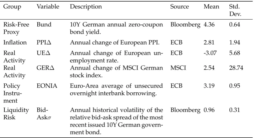
4.2.1 Data Description . . . 22
4.2.2 Regression . . . 24
5.2 Evaluation of Criteria . . . 29
5.2.1 Consistency . . . 29
5.2.2 Intelligibility . . . 30
5.2.3 Availability . . . 32
5.3 Results . . . 32
6 Improvements to the German Government Bond 33 6.1 Credit Risk . . . 33
6.2 Asset Flights . . . 34
6.3 Quantitative Easing . . . 35
6.3.1 Concept of Quantitative Easing . . . 35
6.3.2 Impact of ECB’s Quantitative Easing Program . . . 36
6.3.3 Impact of Foreign Quantitative Easing Programs . . . 38
6.3.4 Adjustment for Quantitative Easing . . . 39
6.4 Proposed Improvements to German Government Bond . . . 40
7 Conclusion 43 7.1 Conclusions . . . 43
7.2 Further Research . . . 44
7.3 Discussion . . . 45
8 Bibliography 47 A Mathematical Derivations 53 A.1 Derivation of the Continuing Value . . . 53
A.2 Derivation of the Consumption Model . . . 53
B Background for Risk-Free Proxies 55 B.1 Interest Rate Swaps . . . 55
B.2 Adjustment to Market Implied Risk-Free Rate . . . 56
C Background for Risk-Free Models 59 C.1 Intertemporal Choice Models . . . 59
C.1.1 Discounted Utility Model . . . 59
C.1.2 Alternative Intertemporal Choice Models . . . 59
C.2 Macro Model’s Additional Data . . . 60
D Detailed Evaluation of Proxies 63 E Public Securities Purchase Program 65 E.1 Concept of Public Securities Purchase Program . . . 65
E.2 Impact of Public Securities Purchase Program . . . 66
E.3 Foreign Quantitative Easing Programs . . . 67
1.1 Thesis Outline . . . 3
2.1 Components of Required Return by Investors . . . 5
2.2 Example of Cash Flows from Risk-Free Asset . . . 5
2.3 Included Financial Risks in Risk-Free Proxy Definition . . . 6
2.4 Components of the Risk-Free Rate . . . 7
2.5 Efficient Frontier . . . 10
2.6 WACC Decomposition . . . 11
3.1 Development of Overnight Rates . . . 15
5.1 AHP Scale of Intensity of Importance . . . 28
5.2 Criteria for Estimator Evaluation with Weights . . . 28
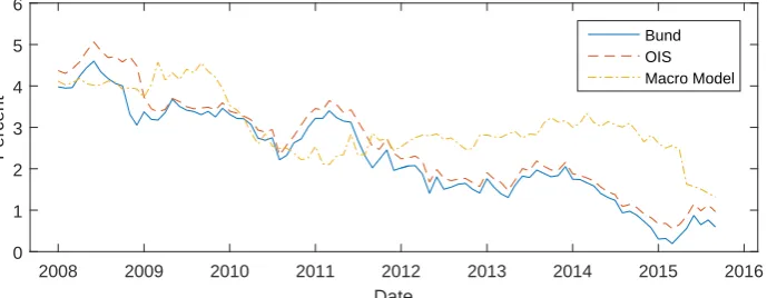
5.3 Development of Risk-Free Estimators . . . 29
5.4 Development of Estimators to Implied Risk-Free Rate Spreads . . . 30
6.1 Bund’s Potential Deficiencies as Risk-Free Proxy . . . 33
6.2 Development of KfW to Bund Spread . . . 34
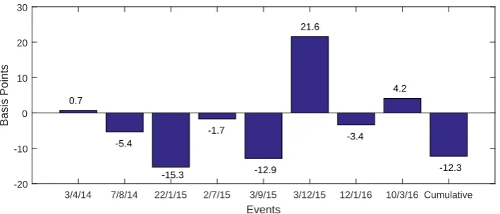
6.3 PSPP’s Cumulative Impact on Bund Yields for Three Time Windows . . . 38
6.4 PSPP’s Impact on the 10Y Bund yield . . . 38
6.5 QE’s Cumulative Impact on the Bund Yield . . . 39
6.6 Bund and KfW-CDS to Market Implied Risk-Free Rate Spreads . . . 41
7.1 Potential Explanations of Negative Real Rates . . . 45
B.1 LIBOR Swap . . . 55
B.2 Transformation of Cash Flows through LIBOR Swap . . . 56
B.3 Market Implied Risk-Free Rate Variants to the Average Risk-Free Proxy Spreads . 56 C.1 Development of Macro-Economic Variables and 10Y Bund Yields . . . 61
E.1 Monthly EAPP Asset Purchases . . . 65
E.2 QE’s Impact Channels . . . 66
E.3 PSPP’s Impact of all Events on 10Y Bund Yield . . . 67
E.4 QE’s impact of all Events on 10Y Bund Yield . . . 68
2.1 Definition of Financial Risks . . . 6
2.2 Drivers of Inflation . . . 8
2.3 Drivers of the Real Rate . . . 9
3.1 Descriptive Statistics of Corporates in our Sample Set from 2008:01 to 2015:12 . . 18
4.1 Historically Implied Discount Factor and CRRA . . . 20
4.2 Variable Description and Summary Statistics from 2000:01 to 2007:12 . . . 23
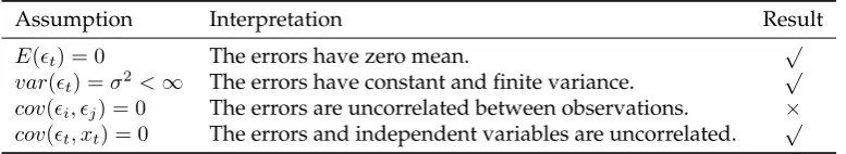
4.3 BLUE Assumptions . . . 25
4.4 Determinants of 10Y Bund Yield from 2000:01 to 2007:12 . . . 26
5.1 Pairwise Comparison Matrix of Evaluation Criteria . . . 28
5.2 Consistency of Risk-Free Estimators . . . 30
5.3 Intelligibility of Risk-Free Estimators . . . 31
5.4 Overall Priorities of Risk-Free Estimators . . . 32
6.1 Overview of International QE Programs . . . 36
6.2 PPSP Announcements . . . 37
6.3 Expected Relative Impact of QE Programs . . . 39
6.4 Impact of QE Programs . . . 39
6.5 Consistency of Bund and KfW-CDS . . . 41
B.1 Cash Flows inemillions from LIBOR Swap . . . 55
B.2 Transformation of Cash Flows through LIBOR Swap . . . 56
B.3 Accuracy of Market Implied Risk-Free Rate Variants . . . 57
C.1 Excluded Variables for Macro Model . . . 62
D.1 Random Consistency Index for Multiple Matrix Sizes . . . 63
D.2 Pairwise Comparison Matrix of Evaluation Criteria . . . 63
D.3 Pairwise Comparison Matrix of Consistency . . . 63
D.4 Pairwise Comparison matrix of Intelligibility . . . 64
D.5 Pairwise Comparison Matrix of Availability . . . 64
E.1 Foreign QE Announcements . . . 68
AHP Analytic Hierarchy Process
BLUE Best Linear Unbiased Estimator
BoE Bank of England
BoJ Bank of Japan
Bund German Government Bond
CAPM Capital Asset Pricing Model
CDS Credit Default Swap
CRRA Constant Relative Risk Aversion
CV Continuing Value
DU Discounted Utility
EAPP Extended Asset Purchase Program
ECB European Central Bank
EONIA Euro Overnight Index Average
EV Enterprise Value
FCF Free Cash Flow
FED Federal Reserve
GC Repo Generalized Collateral Repurchase Agreements
HICP Harmonized Index of Consumer Prices
KfW Kreditanstalt für Wiederaufbau
LIBOR London Interbank Offered Rate
MAE Mean Absolute Error
OIS Overnight Indexed Swap
PSPP Public Securities Purchase Program
QE Quantitative Easing
RMSE Root Mean Squared Error
WACC Weighted Average Cost of Capital
Research Design
We have divided the research design into a conceptual and a technical one, as proposed by Verschuren & Doorewaard (2010). The conceptual part describes the goal of this research. It covers the Problem Context in Section 1.1, our Research Objective in Section 1.2, and the Re-search Questions in Section 1.3. Subsequently, we describe the plan to realize this study in our technical design. It covers our Research Strategy and Thesis Outline in Section 1.4.
1.1
Problem Context
The risk-free rate is the required return on a risk-free asset and is a fundamental concept in finance. A risk-free asset is a theoretical concept and is an asset without any exposure to finan-cial risks. It pays a specified unit in a currency at a certain date in the future in every possible state of the world. The concept has attractive characteristics making it a building block for many finance theories. Fisher (1930) was probably the first to introduce formally the concept to describe the time-value of money. Subsequently, Markowitz (1952) used a risk-free asset’s uncorrelatedness with other assets in Modern Portfolio Theory to construct a portfolio with an optimal risk-return combination. Later, Sharpe (1964) continued on this theory to develop the Capital Asset Pricing Model (CAPM). Finally, Black & Scholes (1973) used the certain return of a risk-free asset in option pricing. We study the risk-free rate in the context of business val-uations. Within this context the risk-free rate is used to construct the Weighted Average Cost of Capital (WACC), which is finally used to discount all expected cash flows of a company to determine its value (Kolleret al., 2010).
In reality no asset fully satisfies all characteristics of a risk-free asset, because it is impossi-ble to eliminate all financial risks (Damodaran, 2010). Therefore the risk-free rate can only be estimated. After a preliminary literature survey we distinguish two risk-free estimator types: proxies and models. Proxies are observable variables and estimate an unobservable variable by closely resembling the theoretical concept (Bai & Ng, 2005). Models consist of several ob-servable variables and are constructed based on theory of a risk-free asset. Currently the most used risk-free estimators are government bonds, resembling the concept due to their assumed absence of credit risk. Governments are regarded as creditworthy, because they can raise taxes and in theory can use monetary policy, i.e., print additional money, to meet their outstanding obligations. However, recently questions have been raised about the adequacy of government bonds as risk-free proxy. This is due to two deficiencies that have been recognized:
• Negative long-term real yields. Currently real yields of several Euro-Area government bonds are negative, when we subtract the inflation expectation from nominal yields (CapitalIQ, 2016). This implies that investors are losing purchasing power over time, contradicting time preference stating that humans prefer direct over delayed consumption (Frederick
et al., 2002). Nominal bond yields require an inflationary and real compensation for bor-rowing money. These components compensate investors for the decrease of purchasing power of the currency and the time-value of money, respectively (Fisher, 1930).
• Increased default risk of governments. Two factors make the negligibility of the credit risk of European government bonds questionable (ECB, 2014). Firstly, Euro-Area governments do not longer have the control of the money supply, because this is transferred to the European Central Bank (ECB). Secondly, the credit risk of European governments has risen significantly after the financial crisis.
1.2
Research Objective
These two deficiencies evoked questions about the adequacy of government bond yields as risk-free proxy. Therefore our objective is to provide recommendations for estimating the risk-risk-free rate for valuation purposes. Firstly, we analyze the most common used proxies, by conducting a literature survey. Secondly, we develop a model as an alternative to the current existing proxies. Subsequently, we evaluate all risk-free estimators on evaluation criteria derived from literature and expert interviews. Finally, we analyze the deficiencies of the best risk-free estimator to further improve its adequacy. The results of this theory-oriented research project contribute to a more adequate estimation of the risk-free rate for valuation purposes.
1.3
Research Questions
To achieve the research objective, we have formulated research questions for structuring our research. Our main research question is:
What is the best estimator of the risk-free rate for valuation purposes?
We have broken down the main research question into four research questions, which are all divided into sub-questions. In this way we are able to research concepts independently and to incrementally answer the main research question.
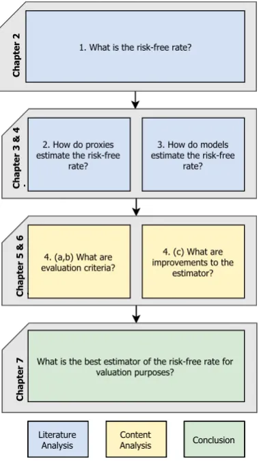
1. What is the risk-free rate for valuation purposes?
(a) What is the risk-free rate from a theoretical perspective? (b) What are components of the risk-free rate?
(c) What function does the risk-free rate have in valuations? 2. How do proxies estimate the risk-free rate for valuation purposes?
(a) Which proxies are used to estimate the risk-free rate for valuation purposes? (b) Why are these proxies assumed to resemble the risk-free rate?
(c) What are the deficiencies of these proxies?
3. How do models estimate the risk-free rate for valuation purposes? (a) What are approaches to model the risk-free rate?
(b) What are weaknesses of these models?
4. How well do the selected methods estimate the risk-free rate for valuation purposes? (a) What are criteria to evaluate estimators from an academic perspective?
(b) What are criteria to evaluate estimators from a practical perspective?
(c) What are improvements to the best estimator of the risk-free rate for valuation pur-poses?
approaches; proxies and models, respectively. Finally, the last Research Question evaluates all estimators for the risk-free rate. As stated previously, in reality no actual risk-free asset exists, so it is impossible to test the adequacy of the proxies directly. To overcome this problem we will formulate evaluation criteria. We will determine these from a theoretical and a business perspective. After the evaluation, we will further analyze the deficiencies of the best method and propose improvements.
1.4
Thesis Outline
FIGURE1.1: Thesis Outline
In our thesis we will use a combina-tion of desk research and interviews for our data gathering. Desk research en-ables us to conduct an extensive analy-sis of the theoretical concepts, making it well suited for the theory-oriented objec-tive of this thesis. Furthermore, this re-search strategy is also very well suited to conduct many similar tests on the prox-ies. We also will conduct interviews con-ducted to provide practical insights for the research.
[image:17.595.330.520.203.540.2]The Risk-Free Rate
In this Chapter we answer the first Research Question by defining and describing the function of the risk-free rate for valuation purposes. Firstly, we deduce from the theoretical concept of a risk-free asset a practical definition of a risk-free proxy in Section 2.1. Subsequently, we describe in Section 2.2 the components for which an investor requires return from a risk-free asset. Afterwards, we describe in Section 2.3 the function of the risk-free rate in valuations. Defining the specific usage in valuations enables us to focus the scope of this thesis. Finally, we synthesize our findings in Section 2.4 by answering the first Research Question.
2.1
Definition
Investors consider investments on a risk-return trade-off. Figure 2.1 shows the components of the required return of an asset by an investor. The required return consists of the return on a risk-free asset, i.e., the risk-free rate, and additional risk premia for financial risks. Hull (2015) defines financial risk as the possibility of financial loss, implying implicitly that the return of a risk-free asset has a standard deviation of zero.
Required Return by Investors
Financial Risks
Risk-Free Rate
+
FIGURE2.1: Components of Required Return by Investors
Thus a risk-free asset always pays a predetermined cash flow. However, the certainty of a specified cash flow does not eliminate all financial risks. In reality investors are bound to a return in a certain currency, inducing the inclusion of inflation and exchange-rate risk. The former is the risk of a greater depreciation of the currency’s purchasing power than initially expected (Bekaert & Wang, 2010). Exchange-rate risk is the risk of the depreciation of the foreign currency in which the return is denominated (Berket al., 2012). Furthermore, this definition also includes liquidity risk, because a predetermined cash flow at a certain date sets no requirements to the ease of trading before maturity. Liquidity risk is the ease with which assets can be sold (Hull, 2015). Concluding, we define a risk-free asset as follows:
An asset paying a specified unit in a currency at a certain date in the future in any possible state of the world.
[image:19.595.224.405.401.466.2]FIGURE 2.2: Example of Cash Flows from Risk-Free Asset
Figure 2.2 shows the cash flows of a risk-free asset with a payoff at year T. It has a single positive cash flow at maturity. This cash flow is certain in every state of the world and is a specified unit, 100+r, in the cur-rency Euro. The present value of the asset is100e, im-plying that the risk-free rate for T years is r/T% annu-ally.
[image:19.595.374.511.652.747.2]In reality no asset guarantees a specified cash flow in any possible state of the world and thus no ‘true’ risk-free asset exists. Therefore, we have to use proxies and models to estimate the risk-free rate. We transform the theoretical definition of a risk-free asset, into a practical definition for a risk-free proxy. We alter the definition to be able to quantify the exposure to financial risks. A practical definition of a risk-free proxy enables us to select risk-free proxies and finally evaluate them. Thus, defining a risk-free proxy is a trade-off between the inclusion of financial risks to make the concept more practical and staying close to the theoretical concept. To understand the considerations in this trade-off, we describe the most common financial risks affecting the cash flow at maturity in Table 2.1. The exposure to and probability of the financial risks differs per asset type, therefore we randomly list the risks. We have excluded interest-rate risk from the overview, because we define this as the resultant of all financial risks.
TABLE2.1: Definition of Financial Risks
Risk type Description Examples
Credit Risk Credit risk arises from the possibility that counterparties may default. Default is the failure to promptly pay financial obliga-tions when due (Hull, 2015).
Bankruptcy or a late interest payment.
Reinvestment Risk
The risk that future cash flows from an as-set cannot not be reinvested at the prevail-ing interest rate when the asset was ini-tially purchased (Damodaran, 2008).
Market interest rate drops during the duration of the loan, so coupons cannot be reinvested at the prevailing rate.
Prepayment Risk
The risk of the early unscheduled return of principal of loans (Damodaran, 2008).
When principal is returned early, future interest pay-ments will not be paid.
Scholars differ over the inclusion of financial risks in defining a risk-free proxy. One group stays true to the strict definition of a risk-free asset, while another only excludes credit risk. We think that controllability is key in deciding in the trade-off for the risk-free proxy. We classify financial risks as either controllable or uncontrollable. Controllable financial risks can be ex-cluded by agreements and uncontrollable financial risks cannot. We classified the three major financial risks in these categories in Figure 2.3. We classify prepayment and reinvestment risk as controllable, because they can be excluded by specific agreements, e.g., a bond can be struc-tured to only include a single payment and no right to early redemption. On the other hand we classify credit risk as uncontrollable, implying the impossibility to completely exclude it. Credit risk cannot be entirely removed, because of the existence of low probability high impact events, e.g., natural disasters.
Concluding, we think it is most accurate for a risk-free proxy definition to exclude all con-trollable financial risks and minimize all unconcon-trollable risks. Hereby we stay as closely pos-sible to the concept of a risk-free asset, but acknowledge the impossibility to exclude uncon-trollable financial risk in reality. Finally, we also stress that our definition of a risk-free asset includes exchange-rate, inflation and liquidity risk. We classify the first two as controllable financial risks, because both can be included by paying in a certain currency. However, we cannot fully include liquidity risk, because we need a certain level of liquidity for efficient mar-ket pricing. Therefore, we require a risk-free proxy to have a sufficient level of liquidity. We regard liquidity above this minimum as an excessive liquidity premium, inflating the price of a risk-free asset. Synthesizing, this leads to the following definition of a risk-free proxy.
An asset paying a specified unit in a currency at a certain date in the future with minimal credit risk and sufficient liquidity.
2.2
Components of Required Return
The risk-free rate is the required return of a risk-free asset by investors. They require compen-sation for postponing consumption and this can be broken down into two elements. Firstly, investors require compensation for the time value of money. Time preference is the economic term describing the preference of humans for direct over delayed consumption (Fredericket al., 2002). This component of the required return is called the real rate. Secondly, investors require compensation for inflation. Investors are not interested in money itself, but in the purchasing power it represents in goods. In order to maintain their purchasing power at the same level, investors require compensation for the expected inflation. This component of the risk-free rate is called the inflation rate. Together both components form the nominal risk-free rate. Fisher (1930) firstly described these components and formalized their relationship at timetbelow. The latter approximation holds when the real and inflation rate are small.
Nominal Ratet= (1 +Real Ratet)∗(1 +Inflation Ratet)−1≈Real Ratet+Inflation Ratet
The equation has become known as the Fisher equation and can be used to decompose the required return in a real and inflationary component ex-post and ex-ante. The ex-post decom-position in hindsight determines the components by using the realized inflation to determine the real rate. Decomposing the required return ex-ante needs forecasts of future inflation and real rates. An inseparable aspect of forecasting returns is uncertainty. Investors dislike uncer-tainty about future cash flows and therefore require additional compensation. This additional compensation is called a risk premium, which is the difference between the expected return from a risky asset and a certain return. In valuing the future real and inflation rate the mar-ket sums the expected rate with the risk premium. According to Fisher (1930) no interest risk premia exist on the long-term, however scholars have shown that they exist on the short-term (Bekaert & Wang, 2010; García & Werner, 2010). Figure 2.4 displays schematically the decom-position of the nominal risk-free rate ex-ante.
Inflation Rate
Expected Inflation
Rate
Inflation Risk Premium Real Rate
Expected Real Rate
Real Risk Premium
Risk-Free Rate
+
+
+
The risk-free rate components determine the required return for a certain period. Of course the length of the period also influences the required return. The relationship between the invest-ment term and the interest rate is called the term structure. The visualization of this relationship is called a yield curve. Generally a longer maturity is accompanied with a higher required re-turn, because a longer maturity is often accompanied with a larger uncertainty, resulting in a higher required risk premia. However, short-term uncertainties sometimes outweigh this effect (Bernothet al., 2012).
2.2.1
Inflation Rate
Inflation is the rate at which the general level of prices for consumer goods and service has risen over a certain period. In the Euro-Area the realized inflation is measured by the ECB with the harmonized index of consumer prices (HICP). This is a price basket of everyday items, durable goods and services weighted by the importance in the household budget (Berket al., 2012). The inflation rate is an important macro-economic variable and therefore is also forecasted. It is forecasted by surveys and mathematical models (Guimaraes, 2012). Important inflation drivers are macro-economic developments and the money supply (Gordon, 1975; Mankiw, 2008). An overview of the main drivers of inflation is listed in Table 2.2.
TABLE2.2: Drivers of Inflation
Driver Description Effect
Demand-pull inflation
Aggregate demand due to increased private and gov-ernment spending.
Demand grows faster than supply, thereby rising the general price level.
Cost-push infla-tion
Drop in aggregate supply. Supply decreases faster than demand, thereby increasing inflation.
Built-in inflation Vicious circle of inflation in-duced by adaptive expecta-tions.
When everyone expects a certain in-flation, the expectation will be incor-porated in the price setting and results in the realization of the expectation. Increase of money
supply
Increased by the govern-ment or central bank.
By increasing the money supply, the general price level increases.
After central banks adapted inflation targeting as policy in the 1990s, the inflation in the Euro-Area has become rather stable. The ECB quantified her objective of price stability in an inflation target of 2%. It uses several monetary instruments to achieve this target. A stable and positive inflation realized that the inflation component of the risk-free was positive and rather stable over the latest years. However, the inflationary compensation does not need to be pos-itive, in case of expected deflation investors can accept a negative inflationary compensation. They accept this, because the purchasing power is expected to grow over time. Since October 2013, the HICP has dropped below 1% and the ECB has taken significant measures to increase inflation. It has set overnight interest rates negative and started the Quantative Easing (QE) program in which it buys government bonds with the goal to stimulate investments. However, until today the measures have not succeeded and the Euro-Area has been exposed to a near zero to negative inflation.
2.2.2
Real Rate
determinant, cyclical factors, is the influence of the short-term interest rates, set by the central banks (Archibald & Hunter, 2013; Cour-Thimannet al., 2006). Table 2.3 summarizes the drivers of the real rate.
TABLE2.3: Drivers of the Real Rate
Driver Sub-driver Description Effect
Neutral Real Rate
Savings and investment equi-librium
The demand and supply equilibrium of the capital markets, determined by the time preference of con-sumers and the investment options.
When the savings demand increases, the equilibrium rate shifts downward.
Impediments to international capital flows
Impediments to capital mar-kets between countries af-fect the equilibrium.
Impediments prevent capi-tal to flow freely between low interest rate countries to high interest rate countries. Cyclical
factors
Adjustments of central banks to lean against in-flationary pressure, also known as the real interest rate gap.
Central banks determine the short nominal interest rate and thereby influence the long-term real rates.
The real rate is an unobservable variable and is can be calculated ex-post with the Fisher equation. Ex-ante the real rate can be estimated by using expectations of the inflation rate or mathematical models to decompose the nominal interest rate. Most of these models are based on the assumption that the high-rated government bonds reflect the nominal risk-free rate. Furthermore the rates of inflation-linked bonds issued by governments are used (Guimaraes, 2012; Canova, 2002).
2.3
Business Valuations
The most used business valuation method is the discounted cash flow method. This method defines the enterprise value (EV) as the net present value of all future free cash flows (FCF). The FCF are the available cash flows to investors and represents the cash that a company is able to generate after setting apart the money required to maintain or to extend its assets base. It is computed by subtracting the capital expenditures from the operating cash flow. The discount rate used in the valuation is the WACC. We show the EV calculation below whereF CFt
repre-sents the FCF at timetandrwaccthe WACC.
EV =
T
X
t=1
F CFt
(1 +rwacc)t
CV = F CFT
rwacc−g
EV =
T
X
t=1
F CFt
(1 +rwacc)t
+ CV (1 +rwacc)T
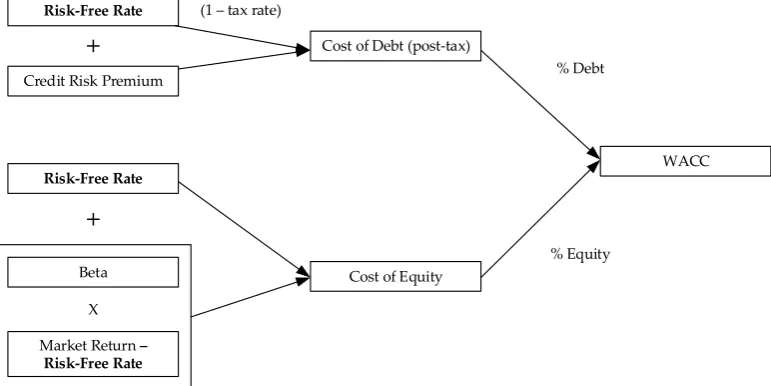
The valuation uses a fixed discount rate instead of a yearly rate. Theoretically a yearly dis-count rate is more accurate, however practitioners use a fixed rate for two reasons. Firstly, the usage of a fixed rate simplifies the valuation, and secondly it causes negligible difference in respect to the yearly method. The maturity of the fixed discount rate is based on duration matching, i.e., matching the duration of the expected cash flows with the duration of a risk-free asset. Generally practitioners use a 10-year risk-free rate when valuing business with an indef-inite horizon (Damodaran, 2008). The WACC represents the minimum return on an existing asset base to satisfy all capital providers. When a company is unable to generate the WACC as the return, capital providers switch to better risk-return investment opportunities. Therefore, the WACC is used as a discount rate. When a company finances itself through equity and debt, then the WACC is calculated as the weighted average of both costs of capital as is shown below. Interest payment on debt can be deducted from taxes and therefore the cost of debt is adjusted for the tax rate (Berket al., 2012). WhereErepresents the total equity,Dthe total debt,Kethe
cost of equity,Kdthe cost of debt, andtthe tax rate.
WACC= E
(E+D)Ke+
D
(E+D)Kd(1−t)
The first component of the WACC, the cost of equity is usually calculated with CAPM intro-duced by Sharpe (1964). It is based on the Modern Portfolio Theory introintro-duced by Markowitz (1952) stating that investors make a trade-off between risk and expected return. Risk in this context is defined as the standard deviation of the possible returns. Investors analyze all in-vestment opportunities and only consider inin-vestments yielding an optimal risk-return trade-off. All investments yielding such a trade-off together form the efficient frontier. This is shown in Figure 2.5 with the reference to ‘previous efficient frontier’.
FIGURE2.5: Efficient Frontier
Modern Portfolio Theory states that inclu-sion of a risk-free asset changes the efficient frontier. A risk-free asset is in this context characterized as an asset with zero risk, im-plying it has a return without any standard deviation. When the simplifying assumption is made that an investor can borrow at the risk-free rate, a tangent through point M, the maximum of the efficient frontier, is created. This line is called the ‘new efficient frontier’ in Figure 2.5 (Hull, 2015). Consider for ex-ample when an investor has an investable amount of 1 and forms an investment i by puttingβiin the risky portfoliomand
invest-ing the remaininvest-ing part 1−βi in a risk-free
asset. This results in the following expected return and risk equations.
E(ri) = (1−βi)rf+βiE(rm)
σi= (1−βi)σf+βiσm=βiσm
the knowledge of the market portfolio in determining the required return for individual invest-ments. His CAPM states that the required return on an investment should reflect the extent to which the investment contributes to the risks of the market portfolio. The common procedure to determine this contribution, is to regress the return of an individual investment to the market portfolio.
ri,t=a+βrm,t+i,t
Whereaandβare constants andis a random variable equal to the regression error. The equation shows that an investment is exposed two uncertain components. Firstly, the compo-nentβrmwhich is the multiple of the market return and referred to as systematic risk. This risk
cannot be diversified away by investing in other investments. Therefore, an investor requires additional compensation for this risk. The second uncertain component,, is non-systematic risk. When we assume that non-systematic risks of assets are independent of each other, then they can be diversified away in a large portfolio. Therefore, an investor does not require addi-tional compensation for non-systematic risk. Concluding, investors thus only require compen-sation for their exposure to systematic and this determines the required return of an individual investment. This asset pricing model is known as the CAPM and shown below.
E(Ke) =rf +β(E(rm)−rf)
The second component of the WACC, the cost of debt, is calculated by summing the risk-free rate with an additional credit risk premium, as shown below. A risk premium is required for the credit risk of a specific company. Credit risk is determined based on publicly known bond rates, credit ratings or a comparison with a peer group. The risk-free rate functions in the cost of debt as a benchmark asset without any credit risk.
Kd=rf+Credit Risk Premium
Figure 2.6 shows the decomposition of the WACC schematically. The risk-free rate has an increasing effect on the WACC, when the asset has a postive beta. Theoretically assets with a negative beta exist, but they are very uncommon. Such companies should profit from negative market returns and vice versa, e.g., restructuring consulting firms and gold. Thus generally an increase of the risk-free rate, when holding everything else constant, increases the discount rate and reduces the enterprise value.
WACC Cost of Debt (post-tax)
Cost of Equity
Risk-Free Rate
Beta
Market Return –
Risk-Free Rate
+
X
Risk-Free Rate
Credit Risk Premium
+
(1 – tax rate)
% Debt
% Equity
[image:25.595.124.510.513.706.2]2.4
Risk-Free Rate for Valuation Purposes
In this Chapter we have reviewed the theoretical concept of the risk-free rate. According to the strict theoretical definition a risk-free asset is not exposed to any financial risk. However, we acknowledge that in reality no true risk-free asset exists and therefore propose a practical definition of a risk-free proxy;“An asset paying a specified unit in a currency at a certain date with minimal credit and sufficient liquidity.”Our definition excludes all controllable financial risks and minimizes all uncontrollable risks. We use our definition of the risk-free proxy to evaluate esti-mators in Chapter 5.
Subsequently, we showed that the risk-free rate consists of an inflation and real compen-sation. The first component compensates for the expected decreased purchasing power of the currency and the second component for the delayed consumption. Humans have time prefer-ence and therefore it is assumed that the real component of the risk-free rate should always be positive. Furthermore, we have shown that several methods decompose nominal risk-free rate into these two components, of which using inflation-indexed bonds is the most used approach.
Risk-Free Proxies
Risk-free proxies closely resemble a risk-free asset and therefore are suitable estimators. In this Chapter, we answer the second Research Question by describing four risk-free proxies. The first and most used risk-free proxies are government bonds, which we describe in Section 3.1. Secondly, we describe Overnight Indexed swaps (OIS) in Section 3.2. Thirdly, we describe gen-eralized collateral repurchase agreements (GC repo) in Section 3.3. Fourthly, we describe our own developed ‘Market Implied Risk-Free Rate’ in Section 3.4. For all proxies we describe their resemblance to a risk-free asset by evaluating their financial risk exposure. Finally, we conclude this Chapter in Section 3.5 by selecting suitable risk-free proxies for valuation purposes.
3.1
Government Bonds
Government bonds are loans issued by national governments with the obligation of periodic coupon payments and the repayment of the face value at maturity. Generally the bonds are denominated in the country’s own currency, but some governments issue also foreign debt for strategic reasons. The government bond yields of the Euro-Area countries differ due to dif-ferences in liquidity and perceived credit risk. The German government bond (Bund) has in general had the lowest yield and therefore we use it as proxy for the Euro risk-free rate. The Bund has a low yield, because of its high liquidity and low credit risk (Ejsinget al., 2015).
Government bonds of developed countries have been used traditionally as risk-free proxy, because of their low credit risk. Governments of developed countries are regarded as cred-itworthy, because of their long-term vision and ability to raise taxes. A conformation of the low credit risk is the high credit ratings of governments of developed countries (CapitalIQ, 2016). Furthermore, governments can in theory use their control over the money supply to meet their financial obligations, i.e., print additional money to pay their creditors (Damodaran, 2008; Dacorogna & Coulon, 2013). However, since the financial crisis in 2008 the negligibility of credit risk of developed countries has been questioned. Credit agencies downgraded several countries and also Credit Default Swaps (CDS) spreads have risen (CapitalIQ, 2016). A CDS provides insurance against the default of a reference entity, and thus indicates the probability of default (Hull & White, 2013). Concluding, the credit risk of developed countries is still low, but certainly not absent.
The government bond market is large with high trading volumes and low transaction costs. Liquidity can be measured in many methods and all indicate a high liquidity of the govern-ment bond market. Fleming (2003) is in favor of using the relative bid-ask spread on assets to measure market’s liquidity and showed that spreads on government bonds are very small. The high liquidity inflates the value of the Bund, distorting it from the price of a risk-free asset requiring only a sufficient liquidity for efficient market pricing.
Finally, government bonds resemble a risk-free asset because of the absence of prepayment and reinvestment risk. Regular government bonds are not callable and include coupon pay-ments (Bloomberg L.P., 2015). The first characteristic means that governpay-ments cannot repay their loan earlier than agreed and thus excludes prepayment risk. Coupon payments exposes government bonds to reinvestment risk. However, coupon-bearing bonds can be stripped to
zero-coupons bonds, which are bonds with only a single payment. The removal of interme-diate payments eliminates reinvestment risk, because the bond has no exposure to fluctuating interest rates until maturity. Synthesizing, we conclude that zero-coupon government bonds have no exposure to prepayment and reinvestment risk and thus resemble a risk-free asset.
3.2
Overnight-Indexed Swaps
An OIS is an interest rate swap based on unsecured overnight interbank borrowing, i.e., all overnight loans between banks without collateral. The Euro OverNight Index Average (EO-NIA) is the average overnight rate in the Euro-Area and is the floating component of the in-terest rate swap. All major currencies have an overnight market, however they slightly differ in construction (Edu-Risk International, 2015). We use the EONIA as example, because it is the overnight rate for the Euro market. To better grasp the concept of an OIS, Subsection 3.2.1 firstly explains an interest rate swap. Subsequently, Subsection 3.2.2 explains the EONIA. Fi-nally, Subsection 3.2.3 describes OIS as risk-free proxy.
3.2.1
Interest Rate Swaps
In a plain vanilla interest rate swap a company exchanges a variable for a fixed cash flow stream or vice versa. It agrees to pay interest at a predetermined fixed rate on a notional principal for a number of periods. In exchange it receives interest of a floating rate on the same notional prin-cipal for the same period. A swap is structured in a way that its net present value at initiation is zero, this means that no cash flows are exchanged at initiation (Hull, 2008).
P V "
YT
t=1
(1 +Floatingt)
−1
#
=P V "
(1 +Fixed)T−1
#
This equation is realized by agreeing to a fixed rate equating the above equilibrium. Thus issuers of an interest rate swap have an expectation of the development of the variable rate. In theory two companies can enter directly into an interest rate swap agreement, but in real-ity each deals with a financial intermediary. Financial institutions act as a market maker for interest rate swaps and provide bid and offer quotes for which they are prepared to exchange floating rates (Hull, 2008). The most common floating rates like the London Interbank Offered Rate (LIBOR) and the EONIA are quoted for maturities up to thirty years.
The structure of interest rate swaps induce a lower credit risk relatively to ordinary loans with the same notional and maturity. Firstly, the creditworthiness of the variable component of an interest rate swap always remain stable. For example the LIBOR rate is always based on A-rated banks and has no risk of declining credit quality. On the other side an ordinary loan to a A-rated bank is exposed to declining credit quality. Secondly, the exchanged cash flows are smaller, because no notional is exchanged and cash flows are netted. The notional itself is only used to calculate interest and not exchanged itself, because it would be meaningless to exchange the same notational at maturity. Furthermore, the cash flows are netted, meaning only the difference between the floating and fixed rate is exchanged. This means that the exchanged cash flows are smaller, reducing credit risk. The netting occurs annually and at maturity (Collin-Dufresne & Solnik, 2001). We show a numerical example of an interest rate swap in Appendix B.
3.2.2
Euro Overnight Index Average
rate at which banks can borrow from the ECB and forms the upper bound of the corridor. The lower bound is thedeposit facility, the compensation banks receive for their overnight deposits of the ECB. The EONIA is always between this corridor, because all panel banks have access to the facilities of the ECB. The corridor is only changed between meeting dates, making EONIA relatively constant between these periods. Figure 3.1 shows the development of the overnight rates (ECB, 2015). The EONIA has sharply decreased after the financial crisis in 2008. Although not entirely clear from the figure, the deposit facility is also below the EONIA in 2014 and 2015.
1999 2001 2003 2005 2007 2009 2011 2013 2015
Date -2
0 2 4 6
Percent
EONIA Deposit Facility Marginal Lending Facility
FIGURE3.1: Development of Overnight Rates
3.2.3
Euro Overnight Index Average Swap
The Euro OIS is an interest rate swap based on the EONIA. The floating rate during an interest period is calculated by compounding the daily EONIA rates. For non-business days the EONIA is not quoted, so it is assumed to remain constant for the non-quoted days. Below we show the calculation of the compounded EONIA for an interest period withTnumber of business days.
Floating Rate=
T
Y
t=1
1 + ntEONIAt 360
!
−1
where nt is the number of calendar days between business day t and the next business
day. According to market European market convention, the interest is calculated based on a year with 360 days, a simplification of reality (Edu-Risk International, 2015). As earlier stated in Subsection 3.2.2, EONIA depends strongly on the corridor set by the ECB, which is only changed at ECB meeting dates. Therefore, EONIA swaps are quoted by market makers based on standard tenors and in short-term also with maturities corresponding to ECB meeting dates. The short-end of the curve is constructed with the assumption that the EONIA remains constant between meeting dates. The longer-end of the curve is constructed by interpolating between quoted maturities.
3.3
Generalized Collateral Repurchase Agreements
A repurchase agreement is a sale of a security with the agreement to repurchase the security at a specified price. Repos are a type of a short-term collateralized loan. We show the calculation of the repo raterbelow. The rate is calculated by determining the difference between the sale price,Ps, and the repurchase price,Pr, for a period withTdays (Hull, 2015).
Ps(1 +r
T
360) =Pr
r T
360 =
Pr
Ps
−1 = Pr−Ps
Ps
r=Pr−Ps
Ps
360
T
A GC repo is a repo type using a predefined basket of safe securities as collateral. The basket primarily contains government and agency securities with the highest credit quality. Agency securities are issued by government agencies and are guaranteed by the central government. Therefore, these securities have the same credit risk as government bonds. GC repos are re-garded to be a risk-free proxy, because they have a low exposure to financial risks. Firstly, credit risk is virtually absent due to the posted collateral. A small credit risk exposure exists, due to the market movements of the collateral, i.e., the collateral can decrease in value. How-ever, this is usually resolved by overcollateralization. Furthermore, GC repos are unexposed to prepayment and reinvestment risk by construction. Their agreement does not include any coupon payments and specifies a fixed repayment date. Lastly, the liquidity of GC repos is very small. The GC repo market is split in overnight and term repos, where the former is highly liq-uid and the latter illiqliq-uid especially for maturities longer than a week (Ejsinget al., 2015).
3.4
Market Implied Risk-Free Rate
Hullet al.(2004) and Blancoet al.(2005) construct a risk-free portfolio by combining a corporate bond and a CDS. We construct a risk-free estimator by averaging many of such portfolios and call it the ‘Market Implied Risk-Free Rate’. We use the term ‘Market Implied’, because it is indi-rectly implied by the market. Firstly, we elaborately explain the concept of the Market Implied Risk-Free Rate in Subsection 3.4.1. Subsequently, we construct the proxy in Subsection 3.4.2. Finally, we review the function of Market Implied Risk-Free Rate as proxy in Subsection 3.4.3.
3.4.1
Concept of Market Implied Risk-Free Rate
A portfolio of a corporate bond and a corresponding CDS is risk-free, because it has no credit risk. The credit risk of the corporate bond is eliminated by a CDS, which we assume to be accurately priced for large corporations. The relationship below should hold, where a holder receives interest from the corporate bond,y, and has to pay the CDS spread,s.
rf =y−s
When the above relation would not hold, then arbitrage possibilities would exist. When for examplesis greater than the difference betweenyandrf, an arbitrageur could make a risk-less
(1999) proposed the following improved estimation of the risk-free rate:
rf =y−s(1 +A)
Most European corporate bonds pay annual interest (CapitalIQ, 2016), so we can determine the expected accrued interest by assuming a certain probability of default of corporates. When we assume consistently with Hullet al.(2004) that the probability of default is uniformly dis-tributed over a year, the expected accrued interestAbecomes y2. In Appendix B we show that the Market Implied Risk-Free variant without the adjustment for accrued interest more accu-rately reflects the risk free rate. We show this by comparing the spreads of the Market Implied Risk-Free variants to the average of the Bund and OIS. We use the latter as benchmark, because they are the only available risk-free proxies for a 5-year maturity. Therefore, in the rest of this thesis we use the variant without the accrued interest adjustment as the Market Implied Risk-Free Rate. Furthermore, our analysis shows that market participants do not value the loss of accrued interest.
3.4.2
Construction of Market Implied Risk-Free Rate
We construct the Market Implied Risk-Free Rate for a 5-year maturity, because of the low liq-uidity of the longer CDS tenors and the low availability of longterm corporate bonds. Annual CDS tenors up to ten years are available, however they are much less liquid for longer maturi-ties. This is shown by the relatively high bid-ask spreads (CapitalIQ, 2016). The low liquidity disturbs accurate market pricing. Furthermore, only a few companies issue 10 year bonds: in our sample period on average 3 companies had 10 year bonds monthly available (Bloomberg L.P., 2015). This forces the Market Implied Risk-Free Rate to be based on only a small group of companies and exposes it to company specific risks. These reasons combined, force us to use only the Market Implied Risk-Free Rate for maturities up to 5 years.
Firstly, we analyzed the Europe CDS index of Markit Group (2015) containing the 125 most actively traded CDSs. We use this index due to its high liquidity. Subsequently, we filtered our selection by two criteria. Firstly, companies must have at least an A S&P rating. Houweling & Vorst (2002) have shown that bond and CDS portfolios of highly-rated companies better reflect the risk-free rate. Secondly, companies must be headquartered in the Euro-Area. This ensures that the majority of their bonds are issued in Euros. This filter resulted in a selection of 29 companies. Subsequently, we obtained for these companies the 5-year CDS spreads and all outstanding bonds from 2008 to 2015 from (Bloomberg L.P., 2015). We only incorporated bonds meeting the following criteria in our sample set:
1. Bonds have to be Euro denominated with fixed coupons. The first component of the criterion makes the loans suitable for determining the Euro risk-free rate. Furthermore, fixed coupons enable us to forecast cash flows.
2. Bonds must not be puttable, callable, convertible or reverse convertible. This ensures that bonds have a fixed maturity and do not incorporate additional risk premiums.
3. Bonds must not be subordinated or structured. These bonds are exposed to different risks than regular bonds.
4. Bonds must be issued publicly, otherwise the market is unable to function efficiently. 5. The amount issued must be at leaste100 million, because large issues ensure sufficient
liquidity.
methods for our data. Both methods show similar outcomes, however the results of the re-gression method have a lower standard deviation. Therefore, we prefer the rere-gression method, because a lower standard deviation indicates more robust results. Three companies had too few bond issues meeting the requirements, so for in total 26 companies 5-year bond yields have been calculated. The Market Implied Risk-Free Rate is determined as the simple aver-age of all companies in the sample. We have used the simple averaver-age, because we consider the assumptions of a risk-free portfolio equally holds for all companies. The descriptive statis-tics of the companies per sector are shown in Table 3.1. The companies are grouped by sector classification of CapitalIQ (2016), because it enables a sector specific review. The most remark-able observation is that the Financials have the largest CDS spread, but their bond yield is not proportionally higher in comparison to the other sectors. A possible explanation is that the Fi-nancials conduct the largest bond issues and so their bonds are traded more actively. Investors prefer this liquidity and therefore require lower bond yields.
TABLE3.1: Descriptive Statistics of Corporates in our Sample Set from 2008:01 to 2015:12
Sector No. Companies Bond Yield CDS Spread
Consumer Discretionary 3 197.31 91.36
Consumer Staples 3 228.14 54.91
Energy 1 250.35 63.61
Financials 11 263.59 119.21
Healthcare 2 213.68 56.65
Industrials 3 216.28 85.45
Materials 3 228.86 57.85
Utilities 3 234.02 73.76
Mean 229.03 76.56
The bond yield and CDS spread are denominated in basis points and are simple averages of the sector. The mean is the simple average of all companies and is used to determine the Market Implied Risk-Free Rate.
3.4.3
Market Implied Risk-Free Rate as Proxy
The Market Implied Risk-Free Rate is a risk-free proxy, because of its low exposure to financial risks and its relative low liquidity. The proxy has virtually no exposure to credit risk, and only a small exposure to reinvestment and prepayment risk. Credit risk is eliminated, because of the CDS in the portfolio. Furthermore, the proxy has a small exposure to reinvestment and prepay-ment risk. The former is caused by the annual payprepay-ments of the CDS premia and bond coupons, inducing intermediate payments. The size of this risk is small, because the payments are in opposite directions and thereby neutralize each other partially. Prepayment risk is caused by the probability of a default, where the face value of the loan is immediately repaid. This forces an investors to reinvest the face value at the then prevailing risk-free rate. The size of this risk is very small, because we only selected A-rated companies having a very low probability of de-fault. Finally, the Market Implied Risk-Free Rate is suitable as proxy, because of its relative low liquidity. The relative bid-ask spread, a common measure of liquidity, is on average four times larger for corporate than for government bonds. However, the spread is still much smaller than non-investment grade bonds (Chenet al., 2007). All these characteristics let the Market Implied Risk-Free Rate closely resemble a risk-free asset.
3.5
Selected Risk-Free Proxies
Risk-Free Models
We answer the third Research Question in this Chapter by providing an overview of the existing methods to model the risk-free rate. We explain the different methods in Section 4.1 and select the most suitable model within the context of this thesis. Subsequently, we construct our own model in Section 4.2.
4.1
Modeling Methods
After a literature review we have selected three risk-free models. The first is based on a con-sumption based asset pricing model and defines the risk-free rate as a function of intertemporal choice. Subsection 4.1.1 describes this ‘Consumption Model’. The second method defines the risk-free rate as a common factor of several market interest rates. The differences between these interest rates are related to specific factors and by calculating these factors we can determine the risk-free rate. Subsection 4.1.2 explains this so-called ‘Co-Movements Model’. The last ap-proach uses macro-economic variables to explain the risk-free rate and we refer to it as the ‘Macro Model’. This method regresses macro variables on a historical accurate risk-free proxy to model the risk-free rate. Subsection 4.1.3 explains this approach in more detail. We conclude this section by selecting the most suitable model for construction in Subsection 4.1.4.
4.1.1
Consumption Model
Campbell (2003) constructed the Consumption Model by defining the risk-free rate as a result of intertemporal choice. Intertemporal choice are decisions involving trade-offs between costs and benefits occurring at different times. Multiple psychological factors have a role in determining a person’s intertemporal choices. Economists have simplified intertemporal choice problems by comparing utility instead of real goods. Utility in this context represents the satisfaction experienced by the consumption of a good. This concept is used, because it is a more universal measure than real goods. The foundation of intertemporal choice is that humans prefer imme-diate over delayed utility. This preference has been translated into a discount function. The intertemporal utility function for the present (t= 0) is given below. In the functionU(Ct)
rep-resents the utility of consumptionCat timet, andD(t)represents the discount function at time
t(Fredericket al., 2002). With positive time preferenceD(t)is a decreasing function and always smaller than 1. We reflect on several discounting models in Appendix C. This reflection has led us to use the discounted utility model in this thesis, as it is the most widely used model.
U =
T
X
t=0
D(t)U(Ct)
The Consumption Model of Campbell (2003) assumes that humans make choices in order to maximize utility over their lifetime. Thus humans equate the cost of consuming one real dollar less at timetand the expected benefit of investing one real dollar in assetiat timetand consuming the dollar and its proceeds int+ 1. He finds this optimum by solving the first-order condition listed below, where the left-hand-side represents the benefit of utility now and the right-hand-side represents the discounted expected benefit of delayed utility. In this function
Et
h
(1 +ri,t+1)U0(Ct+1)
i
represents the expected value of the return of asseti,1 +ri,t+1, and
the derivative of the utility of consumption at timet+ 1,U0(Ct+1).
U0(Ct) =D(t)Et
h
(1 +ri,t+1)U0(Ct+1)
i
Campbell (2003) further specifies the risk-free rate by assuming a certain utility function. He uses the power utility function, which is the most used utility function. Its widespread usage is related to its simplicity and the disagreement on better models. It is simple, because it is the only utility function with a constant relative risk aversion (CRRA) coefficientγ. Risk aversion is the reluctance of a person to accept a uncertain higher expected payoff over a certain lower expected payoff. Besides its simplicity, the power utility has the advantage of being scale-invariant, meaning that is constant over time as wealth increases. The power utility function Campbell (2003) uses, is specified below.
U(Ct) =
Ct1−γ−1 1−γ
Finally, Campbell (2003) defines the risk-free rate, by assuming that the joint conditional distribution of asset returns and the stochastic discount factor is lognormally distributed and homoskedastic. The Consumption model defines the risk-free rate as an asset with a standard deviation of zero, resulting in the specification of the risk-free rate as below. We show the full derivation of Campbell (2003) in Appendix A. This equation states that the risk-free real rate is linear in expected consumption growth, with a slope equal to the CRRA. Furthermore, the variance of the consumption growth has a negative effect on the risk-free rate. Campbell (2003) interprets the latter as a precautionary savings effect, implying that a higher volatility of consumption growth induces more saving.
log(1 +rf) =−log(D(t)) +γEt[∆log(Ct+1)]−
1 2γ
2σ2
m
Weil (1989) was the first to empirically test the Consumption Model with historical data. In his analysis he used the time period ranging from 1889 to 1978. In this period the growth per capita real consumption was 1.83% and the real return on a relatively risk-free security was 0.80%. With the knowledge of these variables only the discount factor and the CRRA are unknown. Weil subsequently implied both variables, by making assumptions about the maxi-mum value of the variables. He capped CCRA at a value of10, the maximum experimentally observed by Mehra & Prescott (1985), and limited the discount factor to.98, implying almost no discounting. The results of Weil (1989) are listed in Table 4.1 and show that both maximum values result in strange implied factors. Firstly, a CCRA of 10 implies a discount factor greater than 1, implying a negative time preference. Secondly, a discount factor of.98implies a CRRA of 29, which is far greater than experimentally observed values (Arrow, 1971). The implied results are very far off from the experimentally observed discount factor and CRRA and thus seem incorrect. Weil (1989) calls this discrepancy between theory and reality the ‘Risk-Free Rate Puzzle’. It poses the question: ‘Why can the risk-free rate be so low with the observed discount factors and CRRA?’ This puzzle is linked to the equity premium puzzle discovered by Mehra & Prescott (1985), questioning the high observed risk equity risk premia with the observed dis-count factors and risk aversion. After the research of Weil (1989), scholars have tried to resolve the Risk-Free Rate Puzzle by altering the utility functions of humans (Kandel & Stambaugh, 1991; Mello & Guimaraes-Filho, 2004), however this has not yet resolved in a solution.
TABLE4.1: Historically Implied Discount Factor and CRRA
rf ∆Ct+1 σc D γ
Concluding, we appreciate the approach of the Consumption Model to model the risk-free rate as a function of human intertemporal choice. It has great explanatory power by linking psychological motives to the risk-free rate. However, the model with the current assumptions has proven to be a bad explainer of the risk-free rate historically. This is as a big disadvantage of the approach.
4.1.2
Co-Movements Model
The Co-Movements Model defines the risk-free rate as the common factor underlying all market interest rates. It interprets market interest ratesriat timetas the sum of the risk-free rate, credit
and liquidity premia and a disturbance term.
ri,t=rf,t+Credit Premiumi,t+Liquidity Premiumi,t+i,t
Reinhart & Sack (2002) and Feldhutter & Lando (2008) propose that besides these four fac-tors market interest rates are also influenced by idiosyncratic shocks, i.e., shocks specific to an asset. For example, they state that government bonds are exposed to these shocks, because they have advantages not shared by other assets, e.g., their widespread use as collateral in repo transactions. The number of unique characteristics in comparison to other bonds determines the exposure to idiosyncratic shocks. Therefore they include an idiosyncratic shock term in the definition of several market interest rates.
The influence of the factors to the market interest rates is quantified with factor loadings. The risk-free rate is assumed to influence all market interest rates equally, i.e., its factor loading is one for all market interest rates. The other factors all influence the interest rates differently. The risk-free rate is solved from the Co-Movements Model by quantifying the factor loadings of market interest rates. This can be done in two approaches, either by determining anchor points or by maximum likelihood estimation. The first method determines specific interest rates as an-chor points without any exposure to specific risks. For example Ejsinget al.(2015) determines the OIS as an interest rate with a zero factor loading to credit risk. When anchor points for all factor loadings have been determined the model can be solved recursively or by regression. The advantage of this method is its ease and intelligibility. However, it has the disadvantage that it relies on arbitrary anchor points. As stated in Section 2.1, in reality no assets without credit or liquidity risk exposure exist, so by definition these anchor points are only approximations. The second approach in solving the factor loadings uses maximum likelihood estimation. This approach determines the factor loadings by calculating the maximum likelihood of the factor loadings within a selected set of interest rates, which can be done with various techniques. The advantage of this method is that it does not rely on subjective methods, however it does require complex maximum likelihood estimators.
The main advantage of the Co-Movements Model’s approach to model the risk-free rate is its economic interpretation. It isolates risk premia in existing market interest rates to determine the risk-free rate. Thereby it let risk-free proxies more closely resemble a risk-free asset. How-ever, the biggest disadvantage of the model lies within the determination of the factor loadings. The first approach relies on subjective anchor points decreasing the accuracy of the model. This is caused by the fact that these anchor points are per definition approximations. Furthermore, the second other approach uses complex maximum likelihood estimation methods decreasing the economic interpretation and are outside the scope of this thesis.