Linking subjective mental workload to performance on bronchoscopy simulator tasks

(1)

simulator tasks

Luise Warnke University of Twente

Department of Cognitive Psychology and Ergonomics

Bachelor thesis

Author Note

Date: June 27, 2018

(2)

Abstract

Introduction: In selection of future pulmologists a differentiation needs to be made between those who will reach a high performance level and those who will not. By combining mental workload and performance measures we aimed to get better predictions of maximal performance individuals will reach.

Methods: Thirteen students participated in training on a 3D-Systems GI-BRONCH Mentor simulator. The training was split in two sessions consisting of a total of three tasks teaching basic bronchoscopy skills. Performance was recorded by the simulator and the NASA-TLX was filled in between the trials. Both measures were to be modeled as learning curves and their asymptotes correlated.

Results: Due to insufficient representation of NASA-TLX scores as learning curves they were not compared to performance scores. Based on exploratory plots, data was found to fit third degree polynomials well.

(3)

1 Introduction

One of the major breakthroughs in modern medicine was the development of procedures that do not require open surgery, so called Minimally Invasive Procedures or Surgery (MIS). These procedures enable physicians to examine, sample and repair tissue in narrow tracts of our bodies without causing major injury. At the same time, risk of post-surgical infections is reduced (Dobson et al., 2011).

The price for reduced risk for patients is higher challenges for physicians. Unlike open surgery, MIS does not give direct visual and haptic contact with the operation area and tools. Information not perceived directly has to be filled in from memory or imagination, processes that put additionally cognitive load on the operator. And indeed a lack of sensory input has been found to be correlated with higher mental workload (MW) during several tasks, including MIS (see for example Berguer, Smith, & Chung, 2001; McCarley & Wickens, n.d.; Yurko, Scerbo, Prabhu, Acker, & Stefanidis, 2010.

But not all persons are alike in what gets the mentally loaded and in how much they perceive a task as loading. In general, those who are more loaded by a task do also perform worse, a condition that is maleficent during medical procedures. Through the combination of performance and MW measures we therefore hoped to differentiate novices on how good their final training outcome will be.

For training a bronchoscopy simulator was used. We initially planned to analyse the collected data through a learning curve model - which is discussed below - but exploration of the MW data was strongly contradicting this model and therefore analysis eventually was based on another model. A factor that might have caused this unexpected result, might have been that due to material breakage less data was collected than planned.

Nevertheless, in the following sections our initial expectations will be discussed. First, we give an introduction to bronchoscopy. Then the model used for analysis will be described in more detail and it will be explained how measures of MW can be integrated into it.

1.1 Bronchoscopy and training of pulmologists

(5)

to flexible endoscopes which can be brought to deep bronchi without causing severe injury (for a discussion on the history of bronchoscopy see Panchabhai & Mehta, 2015).

To conduct bronchoscopy a pulmologist stands by the head of patients laying on their back. The bronchoscope is introduce through the mouth or nose using the non-dominant hand while the control tool is held in the dominant hand. The scope can be moved up and down by a lever on the tool and rolled left and right by turning of the wrist. During the process the pulmologist needs to keep track of various motor tasks, like avoiding the scope from bending and maintain a certain body posture. Additionally, assistants need to be coordinated and anatomical knowledge has do be retrieved. This factors make the procedure demanding in several ways.

Special courses are provided for physicians who want to qualify for the procedure. These courses differ in length and end examination. Konge et al. (2012) reasoned that this comes through an absence of a valid criterion for expertise.

And indeed there are courses as the one offered by the American College of Chest Physicians (CHEST) which is not set to an exact duration but all parts need to be finished within three years (CHEST, 2018). Also, they do not refer to an evaluation form but state they award a Certificate of Completion to those who “meet the performance, proficiency, or passing standard for the assessment(s)” (CHEST, 2018, para. 5).

Other countries actually do provide information on training duration and criteria for proficiency. Training of prospective pulmologists in the Netherlands, for example, is standardized by the Nederlandse Vereniging van Artsen voor Longziekten en Tuberculose (NVALT). The complete specialisation process is set to take six years and is organized in modules, that focus on different aspects of the work as a pulmologist and different procedures used. (NVALT, 2017). The final evaluation of the bronchoscopy module is done using the Bronchoscopy Skills and Tasks Assessment Tool (BSTAT). On the BSTAT a maximum of 100 points can be achieved whereof 19 account for scope handling; the rest is given for orientation and identification ability (Bronchoscopy International, 2010).

(6)

examinators who have differing standards; one might give the 5 points when the scope is centered most of the time, another might not give them even if centering was not kept for only a short time.

Another approach to standardisation was examined by Konge et al. (2012). They aimed to identify the number of surgeries needed to reach proficiency and found 80 surgeries to be sufficient. Still, there is the possibility that trainees will not have reached proficiency after that time - in this study that was the case for 1 in 28 physicians - or reach proficiency earlier (also 1 in 28). As time and money may be wasted on additional training it seems more fruitful to determine how much training is necessary early on in training.

Both of these problems, lack of objective rating and differences in training sessions needed, can be approached through the usage of simulators in examination. It already has become good practice to use simulators during the training process since they can be used for self-administered practice (Gopal et al., in press) and can be used to train single aspects of a procedure (Schreuder, Oei, Maas, Borleffs, & Schijven, 2011). But simulators do also record performance data which can be used to provide objective feedback. This feature is already being used in the training of CHEST (Simbionix, n.d.).

Predicting the right amount of training proves to be a harder challenge. Through the usage of simulator output learning curves can be calculated. But, when only based on performance data, predictions have a high degree of uncertainty, especially early in training. Through integration of measures as MW- which will be discussed shortly - we hope to gain certainty earlier. But first we will turn to the learning curve model.

1.2 Predicting future performance from learning curves

To establish an efficient selection method for those who will reach proficiency in MIS, learning curves from prospects completing simple tasks on simulators can be analysed. This has the advantage that less repetitions are needed than the 80 as proposed by Konge et al. (2012) and therefore time is saved. Also the same simulators as those used in training can be used for selection and therefore no additional costs incur.

(7)

Figure 1. Learning curve of Participant 6 on Task 3. The rate of curvature describes the maximal change, the asymptote the maximal level of performance that will be reached and the amplitude the difference between initial performance and asymptote.

from the best expected performance or in other words: how much someone learns. The rate of change indicates the speed of learning; a high rate of change means that the individual was quicker in reaching the final performance than someone with a low rate of change. Finally, there is the asymptote. This is the value corresponding to the best performance that will be reached by a person and therefore is what we are interested in when predicting whether someone will reach proficiency.

Dissenting from traditional statistics the focus during analysis of learning curves clearly lies on individual performance (Brown & Heathcote, 2003). After all, we want to know whether individuals will be good pulmologists and not whether the group on average will be good pulmologists, risking a wide spread between very good ones and very bad ones.

(8)

have not been of strong support for any of these assessment methods it is still being looked for a measure that helps to predict performance. With this study we want to give it another try to tackle the question by the use of mental workload measures.

1.3 Mental Workload and Task Performance

Mental Workload is a factor that is deeply interrelated with performance, experience and learning. It determines performance by allocating resources, but also does performance determine mental workload as bad performance calls for adaptation (Parasuraman & Hancock, 2010).

According to Wickens’s (1980) influential Multiple Resources theory each of our senses has a finite amount of cognitive resources available to one process (e.g. object recognition) at a time. Several objectives might involve usage of one resource in conflicting ways (Wickens, 2002). During bronchoscopy conflicts may for example be caused by the need to identify the distance to the next airway junction as well as estimating space left to the sides of the scope. Both of these objectives involve distance inference but one in depth, the other in width.

When conflicts arise processing is delayed or imprecise, causing unforeseen events that ask for responses that do not belong to the main workflow. These off-task responses lead to a sudden increase in information to be processed which according to Parasuraman and Hancock (2010) is what is actually perceived as high load and interferes with performance. For example, in the task used for the study at hand contact between the bronchoscope and the airway walls caused auditory and visual feedback that prompted the operator to reject the scope, an activity contrary to the main task of inserting the scope. These spontaneous actions are less proficient in execution and therefore can lead to more injuries being caused to the patient (Yurko et al., 2010).

(9)

increase of performance scores) and internally in automatization (i.e. decrease of mental workload; Zheng, Cassera, Martinec, Spaun, & Swanström, 2010).

In a good learning process we should should expect automatization and learning to develop parallelly; techniques that cause good performance should be automatisized. And Stefanidis, Scerbo, Montero, Acker, and Smith (2012) actually found that performance was better when the goal of training was reaching automatization gather than reaching proficiency. Therefore the level of automatization can also be used as a measure of performance. If this is true, performance scores and mental workload scores handed to a learning curve model give more precise predictions of the asymptote as either of the two on their own. This should become visible as a high correlation of their asymptotes (Arendt, 2017).

1.4 Measuring Mental Workload

Even though there has been an increase of physiological methods to measure MW as for example heart rate variability which are reliable (Jorna, 1992), subjective measurement is still often the method of choice. Especially in environments where subjects need to perform a physical task the instrument might interfere with task performance. Two instruments used often are the Subjective Workload Assessment Technique (SWAT; Reid & Nygren, 1988) and the National Aeronautics and Space Administration Task Load Index (NASA-TLX; Hart, 1986).

In a meta-analysis de Winter (2014) found that the SWAT has been used 825 times and the NASA-TLX almost 7,000 times in published papers. So both have a sufficient amount of results for comparison and validation (see for example Hill et al., 1992). But de Winter (2014) uttered concerns that the NASA-TLX only came to be used that often due to its high popularity and not due to advantages as found by Hill et al. (1992). Still, we are concerned that the SWAT lacks sensitivity for the given situation as it only uses Time Load, Mental Effort and Psychological Stress but does not include physical aspects of the performed task (Reid & Nygren, 1988). Also scales are not continuous but using a three level design, from high to low.

(10)

Unfortunately, the tool has not been used often at the moment of writing and validity might not be sufficient. Because we used a new design, we wanted to avoid eventual effects caused by an invalid instrument. For the given reasons we prefer the NASA-TLX over the other two.

Within the field of MIS several studies exist that used the NASA-TLX. Within this research two different goals can be identified. The first is the development of supportive technologies. By employing the NASA-TLX it was shown, for instance, that three-dimensional displaying is less stressing for physicians than traditional two-three-dimensional displaying (Foo et al., 2012; Gómez-Gómez et al., 2015).

A second goal is to improve selection and training of physicians. For example, Yurko et al. (2010) found NASA-TLX scores to significantly correlate with performance scores measured at three moments of training and O’Connor, Schwaitzberg, and Cao (2008) showed that providing results and instruction helps to lower MW for trainees. The study at hand belongs to this latter field of research with the novelty of linking NASA-TLX scores to concurrent performance to get better insight in its relation to learning of MIS.

2 Methods

2.1 Design

The study was designed two measure performance, as Time on Task (ToT), and MW, as NASA-TLX scores. Those to measures were collected on three times 15 data points. Scores were to be correlated.

2.2 Procedure

(11)

The first task taught basic scope manoeuvres. The scope was to be moved through a virtual reality (VR) tube system while keeping an indicator at the middle of the screen (Figure A1). If the scope touched the walls participants were warned by visual and auditory feedback. Fifteen tracks were followed in total. Beginning from the first trial, the NASA-TLX was filled in every second trial. Participants needed an average of 33 minutes to fulfil the first task.

After a break of five minutes the participants continued to the second task. Now they needed to perform a lung inspection by searching for light bulbs which were situated at the major airway junctions (Figure A2). Of the 28 light bulbs available 10 needed to be found and matched to an on-screen indicator. Again this was repeated 15 times and the procedure for the NASA-TLX as in Task 1 was followed. The second task took on average 47 minutes.

After the training was finished the participants were thanked for attending and asked whether they had any more questions and whether they were willing to participate in a second session. The first session was set to last for a maximum of two hours.

For the second session the participants returned on another day. Upon arrival they were shown a video explaining the usage of sampling tools. Again participants had the chance to ask questions and then started with the third task. This time they had to perform a tissue sampling task. The spot of interest was marked in a purple colour in the simulated lung (Figure A3). To obtain the sample the tool was handed over by the researcher and then had to be introduced through the bronchoscope’s working channel. At a certain level of insertion the simulator prompted to choose one of several sampling tools from the screen. First, the participant had to choose a forceps. After doing so, they were handed the tool handle to their non-dominant hand. The sample was obtained by either pushing the handle up or down while holding the scope at the sampling area.

When the sampling was successful the tool needed to be rejected until the selection panel would be shown again. Then the sampling brush had to be chosen. A second sample was obtained by moving the tool back and forth in the working channel. After this second sampling was successful the trial was finished. The third task was also repeated 15 times and the NASA-TLX again was filled in after every second trial. This resulted in an average time of 47 minutes.

(12)

the experiment. The second session was set to a maximum time of one hour. Neither for the first nor the second session was maximum time exceeded.

Pre- and pilot test. Prior to writing the protocol used, the tasks were pretested by the researchers. The goal hereof was to find out how long each trial of the simulator tasks will take and to get comfortable with the apparatus used. Also it was concluded to provide stools for smaller participants since the table’s height could not be changed and was considerably high.

The resulting protocol was pilot tested on a 21 years old male, Dutch student of Medical Healthcare and Technologies. The procedure did not exceed the set maximum time of two hours and proofed to be expedient. Analysis of the data recorded during the pilot test indicated that completion of the NASA-TLX after every second trial was sufficiently resembling its progress. So this was preferred in order to cut down session time.

2.3 Measures

Simulator. As the simulator used is designed for education and not for research the recorded data did not satisfy our criteria. Therefore it was decided to include the following measures in the analysis.

For Task 1 the ToT as measured by the simulator was used. Because routes were drawn at random from a list of 8 routes, also the corresponding route number was recorded. This enabled us later to check for eventual differences in difficulty of routes.

For Task 2 and 3 also ToT was used in the analysis but the output from the simulator differed from the actual times. Therefore times were manually stopped by the researchers, starting at the moment of scope insertion and stopping when the final criterium - for Task 2 identification of the tenth light bulb and for Task 3 finishing sampling with the brush -was met. Additionally, during Task 2 the times were recorded between the single light bulbs and during Task 3 the time needed for both of the sampling procedures. Full lists of variables measured by the simulator are provided in Appendix B.

(13)

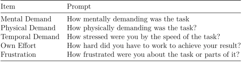
Table 1

Prompts to the different item as provided on-screen

Item Prompt

Mental Demand How mentally demanding was the task Physical Demand How physically demanding was the task?

Temporal Demand How stressed were you by the speed of the task? Own Effort How hard did you have to work to achieve your result? Frustration How frustrated were you about the task or parts of it?

Note. Questions adapted from Hart (1986, Appendix A).

item was omitted. The other five were displayed as continuous scales ranging 0 to 100 (see Figure C1).

At the beginning of both sessions on-screen information was provided on how the survey should be taken. Participants were asked to judge from intuition and focus on the preceding trial and not the overall performance. Also prompts to the items as provided in Table 1 were given.

Hart (1986) included a card sorting task through which it can be measured which factor subjectively impacts MW the most. We implemented the card sorting as a drag-and-drop ranking which was done after finalizing all trials of each task (see Figure C2). Each item was assigned a rank from 1 to 5. No rank could be assigned two times. For the ranking participants were asked to judge all trials they performed.

2.4 Data analysis

As well performance scores as NASA-TLX data were analysed using an adapted version of the model proposed by Heathcote, Brown, and Mewhort (2000). The basic model is represented by Equation 1. Before performing analysis scores were transformed to lay within an interval from 0 to 1, as it is good practice. Finally, correlations between the asymptotes of performance and NASA-TLX were to be calculated, to answer our research question.

P erf ormance= exp(Amplitude−exp(Rate)×NT rial) + exp(Asymptote) (1)

[image:13.595.102.499.108.209.2]

(14)

T LX = 5 X

i=1

Scorei×Ratingi

15 (2)

The analysis was conducted using the statistics-focused programming language R and the Bayesian Regression Models engine (brms; Bürkner, 2017). The code is given in Appendix D.

2.5 Material

Simulator. The simulator used was a GI-BRONCH Mentor produced by 3D-Systems. It consists of a hard-plastic body with openings for as well bronchoscopy as gastrointestinal endoscopy. The system was connected to a touchscreen that was placed just above the body and could be turned to face the operator.

The bronchoscope was controlled using a handle as shown in Figure A4a. The scope’s tip could be bowed by pushing the lever up or down. Side ward rotation was achieved by rotation of the whole handle from one’s wrist. The tool shown in Figure A4b could be introduced through the scopes working channel and used by the attached handle.

The tasks were included in the BronchMentor training curriculum for prospective pulmologists (Simbionix, n.d.). Also was a video included in the MentorLearn software1 used to explain basic bronchoscope handling. For explanation of the third task a self-produced video was used2.

Laptop. The NASA-TLX as well as the demographics survey were displayed on the researchers’ laptops. They were accessible online at Qualtrics using an anonymous link.

Intake Questionnaire and Informed Consent. Basic demographic data of participants was collected. In addition it was asked for weekly gaming time in accor-dance with studies showing a positive correlation between gaming and MIS performance (Enochsson et al., 2004). Also participants were asked to indicate whether they had any visual or motor disabilities which would hinder them from proper performance. The questions used are shown in Appendix E. Informed consent was given on a paper form as presented in Appendix F.

1_{Included as “Posture and Scope Maneuvering”}

(15)

2.6 Participants

We initially aimed at a sample size of 25 but due to breakage of the bronchoscope we had to stop data collection early. Eventually, twelve students of the University of Twente and one of the Saxion University of Applied Sciences participated in the study, resulting in a total sample of 13. Five participants attended both sessions.

Nine of the students were recruited using the university’s research pool and received two European Credit Points as a reward of the first session and one more for the second session. The other four participants were a convenience sample.

The convenience sample consisted of three male and one female Dutchmen. Two ma-jored in Mechanical Engineering, the other in Applied Physics and Industrial Engineering, respectively. The sample from the research pool consisted of one male and eight females. Again eight were German and the other Bulgarian. Six were majoring in Psychology and three in Communication Studies.

The total sample’s age average was 20.2 years ranging from 19 to 23. Two out of thirteen described themselves to be left-handed. Three of the participants indicated to be playing video games on a regular basis with an average of 11.3 hours of gaming per week. None of the participants needed to be excluded from analysis due to impairments.

3 Results

Performance was found to be learning curves (Appendix G), but our expectation that the NASA-TLX scores also take that shape and, thus, their asymptotes correlate with those of the performance learning curves did not hold. Instead we observed the NASA-TLX scores best to be fit by a polynomial of third degree. As through this development MW was not compared to performance scores, the latter is not described here, but analysis can be found in the thesis of Marlise Westerhof (In Progress).

Through the first analysis of the total scores of the NASA-TLX it turned out that they did not take a shape resembling a learning curve when mapped against the trials (Figure 2). While participants 6, 10 and 13 show a clear decrease of MW and participants 8,9 and 12 show irregular progression, the rest remains at the initial level of MW. Participant 2 was excluded from this first analysis since due to technical problems they could not complete the ranking.

(16)

Figure 2. Total NASA-TLX scores as calculated from Equation 2. Each subfigure corresponds to one participant. Lines are smoothed using locally weighted scatterplot smoothing (LOESS).

showed a high consistency (α = 0.84). Task 3 was excluded from further analysis as only little data was collected. Through analysis of plots like the one shown in Appendix H, three types of development could be identified. It could be found that some individuals show a decrease in MW while others maintain their initial level. But for most participants workload increased after an initial decrease.

(17)

T LX = 3 X

i=0

aixi =a0 +a1x+a2x2+a3x3 (3)

Applying the polynomial model resulted in the curves shown in Figure 3. From these curves it seemed that the model better matches data from the second task than from the first task. Those of the first task did not yield the characteristic maximum in the beginning. This difference is very good visible for Participant 2 and 13.

Figure 3. Representation of the NASA-TLX scores as third degree polynomials. Task 3 was excluded from analysis due to small sample size.

(18)

mean of Mr <0.00. Confirming our observation made from the model plots Figure 3, Task 2 was fitted slightly better than Task 1 (r2 _{= 0.21;} _r2 _{= 0.29, respectively).}

From the given plots it can also be observed that minima and maxima are positioned similar across all participants (see Figure 3). For Task 1 the point of change can be found at about 11 trials; for Task 2 the maximum lies at about 4 trials and the minimum at about 12 trials. What actually differs between individuals is the range of scores. A very prominent example hereof is Participant 6 whose scores have a range of about 20 points for both tasks.

4 Discussion

It was expected that mental workload as measured by the NASA-TLX can be used together with performance data measured by a training simulator for bronchoscopy, to give improved predictions of maximal performance individuals can reach. This would have been possible if as well performance as mental workload had taken a learning curve shape. Unfortunately, no such shape was found. We rather found that, after a short period of increase, scores would decrease, to finally increase again. Following this observation we modeled the data to a third degree polynomial.

This shape of curvature might be interpreted as phases corresponding to the different uses of MW measurement (see Figure 4). This does not mean that each of these phases is limited to a certain time; rather these processes happen in parallel but one prevails at a certain time resulting in the curvature.

The first phase is overload or stress. The novelty of the task causes inefficient filtering of information, interference of cognitive processes and erroneous choice of response. This phase matches to the classical notion of MW as Wickens (1980) used. The second phase can be described as automatization, the process we were initially interested in. In this phase efficient methods for handling and cognitive processing are chosen to lower the initial stress (Parasuraman & Hancock, 2010). For the third phase we found two competing explanations with crucially different implications. They will be discussed in turn.

(19)

Figure 4. Polynomial curve of NASA-TLX scores of Participant 1 on Task 2 with the phases discussed. The first phase is interpreted as stress, the second as automatization, and for the third arguments for an interpretation as either fatigue or increased effort is provided.

In conditions were vigilance has to be maintained performance is starting to decrease through fatigue after about 30 minutes (Mizuno et al., 2011). Based on the measured times (see subsection 2.2) this would indicate that as off the tenth repetition fatigue was setting in for our participants, but through the data it seems that automatization prevails for 2 more trials. As a state of fatigue is associated with lowered ability to maintain motivation and lowered cognitive ability which will be restored after a period of rest (Mizuno et al., 2011), this interpretation implicates that a break should be given to trainees when mental workload rises.

Another explanation might be that after the process is automatized more effort is put into the task to increase performance. Fairclough (2010) argued that the uppermost goal of a human performing a task is to perform good. The will to do so is restricted by the need to maintain a comfortable level of MW. This means that if stress is above one’s level of comfort when learning a new task, one needs to wait for the stress to decrease through automatization before being able to put more effort in it to reach ones actual goal (i.e. perform good). From this perspective it would be logical to focus training on the third phase because this is the phase where the trainee is striving for perfection.

(20)

of the SWAT, actually used polynomials to model their data but eventually found an additive model to better fit their data.

We did not expect to find these results and have to consider that they are caused by major deficits in the design. Especially, the low number of participants that causes high uncertainty of the model but also the missing data for every second trial can be considered contributing factors. Still, the deviation of the expected model is so essential that a replication of the study without these shortcomings would be interesting.

Another point regarding the method that needs to be discussed is the usage of the NASA-TLX. Our analysis showed that for the tasks performed all subscales of the NASA-TLX showed a high correlation. It can be recommended for similar studies to use single item tools like the Overall Workload (OW) scale developed by Vidulich and Tsang (1987) which shows similar validity and usability as the NASA-TLX (Hill et al., 1992) with the advantage of decreased time demand and less effort asked of the participant. Through the usage of a one-item scale it would even be reasonable to ask for response after every trial. This would still result in a decrease of asked responses by more than 60 %.

(21)

References

American College of Chest Physicians. (2018). Certificate of Completion. Retrieved from http://www.chestnet.org/Education/Advanced-Clinical-Training/Certificate-of -Completion-Program

Arendt, A. (2017). Towards reliable and valid predictionof MIS-performance with basic laparoscopic tasks in the LapSim and low-fi dexterity tasks (Master thesis). University of Twente, Enschede, The Netherlands.

Baldwin, C. L., & Reagan, I. (2009). Individual Differences in Route-Learning Strategy and Associated Working Memory Resources. Human Factors,51(3), 368–377. doi: 10.1177/0018720809338187

Berguer, R., Smith, W. D., & Chung, Y. H. (2001). Performing laparoscopic surgery is significantly more stressful for the surgeon than open surgery. Surgical Endoscopy, 15(10), 1204–1207. doi: 10.1007/s004640080030

Bronchoscopy International. (2010). Bronchoscopy Skills and Task Assessment. Retrieved from https://www.bronchoscopy.org/education/PDFS/BEP/BEP%20Assessment% 20Tools/BSTAT.pdf

Brown, S., & Heathcote, A. (2003). Averaging learning curves across and within participants. Behavior Research Methods, Instruments, & Computers,35(1), 11–21. doi: 10.3758/ BF03195493

Bürkner, P.-C. (2017). Brms: An R Package for Bayesian Multilevel Models Using Stan. Journal of Statistical Software, 80(1). doi: 10.18637/jss.v080.i01

de Winter, J. C. F. (2014). Controversy in human factors constructs and the explosive use of the NASA-TLX: A measurement perspective. Cognition, Technology & Work, 16(3), 289–297. doi: 10.1007/s10111-014-0275-1

Dobson, M. W., Geisler, D., Fazio, V., Remzi, F., Hull, T., & Vogel, J. (2011). Minimally invasive surgical wound infections: Laparoscopic surgery decreases morbidity of surgical site infections and decreases the cost of wound care: Minimally invasive surgical wound infections. Colorectal Disease,13(7), 811–815. doi: 10.1111/j.1463 -1318.2010.02302.x

(22)

874–880. doi: 10.1016/j.gassur.2004.06.015

Fairclough, S. H. (2010). Mental Effort Regulation and the Functional Impairment of the Driver. In P. A. Hancock & P. A. Desmond (Eds.), Stress, Workload, and Fatigue (pp. 479–502). Mahwah, NJ: Lawrence Erlbaum Associates.

Foo, J.-L., Martinez-Escobar, M., Juhnke, B., Cassidy, K., Hisley, K., Lobe, T., & Winer, E. (2012). Evaluating Mental Workload of Two-Dimensional and Three-Dimensional Visualization for Anatomical Structure Localization. Journal of Laparoendoscopic & Advanced Surgical Techniques,23(1), 65–70. doi: 10.1089/lap.2012.0150

Gómez-Gómez, E., Carrasco-Valiente, J., Valero-Rosa, J., Campos-Hernández, J. P., Anglada-Curado, F. J., Carazo-Carazo, J. L., . . . Requena-Tapia, M. J. (2015). Impact of 3D vision on mental workload and laparoscopic performance in inexperi-enced subjects. Actas Urológicas Españolas (English Edition), 39(4), 229–235. doi: 10.1016/j.acuroe.2015.03.006

Gopal, M., Skobodzinski, A. A., Sterbling, H. M., Rao, S. R., LaChapelle, C., Suzuki, K., & Litle, V. R. (in press). Bronchoscopy Simulation Training as a Tool in Medical School Education. The Annals of Thoracic Surgery. doi: 10.1016/j.athoracsur.2018.02.011 Groenier, M., Schmettow, M., Huijser, S., & Gallagher, A. G. (n.d.). Predicting laparoscopic

skill aquisition. Unpublished manuscript.

Hancock, P., & Verwey, W. (1997). Fatigue, workload and adaptive driver systems.Accident Analysis & Prevention, 29(4), 495–506. doi: 10.1016/S0001-4575(97)00029-8 Hancock, P. A., & Chignell, M. H. (1988). Mental workload dynamics in adaptive interface

design. IEEE Transactions on Systems, Man, and Cybernetics, 18(4), 647–658. doi: 10.1109/21.17382

Hart, S. G. (1986). Task Load Index: Computerized Version (Tech. Rep. No. 20000021487). Moffett Field, CA: NASA Ames Research Center.

Heathcote, A., Brown, S., & Mewhort, D. J. (2000). The power law repealed: The case for an exponential law of practice. Psychonomic Bulletin & Review, 7(2), 185–207. doi: 10.3758/BF03212979

Hill, S. G., Iavecchia, H. P., Byers, J. C., Bittner, A. C., Zaklade, A. L., & Christ, R. E. (1992). Comparison of Four Subjective Workload Rating Scales. Human Factors, 34(4), 429–439. doi: 10.1177/001872089203400405

(23)

of its validity as a workload index. Biological Psychology, 34(2-3), 237–257. doi: 10.1016/0301-0511(92)90017-O

Konge, L., Clementsen, P., Larsen, K. R., Arendrup, H., Buchwald, C., & Ringsted, C. (2012). Establishing pass/fail criteria for bronchoscopy performance. Respiration, 83(2), 140–146. doi: 10.1159/000332333

McCarley, J. S., & Wickens, C. D. (n.d.). Human factors concerns in UAV flight. https:// www.faa.gov/about/initiatives/maintenance_hf/library/documents/media/ human_factors_maintenance/human_factors_concerns_in_uav_flight.doc.

Mizuno, K., Tanaka, M., Yamaguti, K., Kajimoto, O., Kuratsune, H., & Watanabe, Y. (2011). Mental fatigue caused by prolonged cognitive load associated with sympathetic hyperactivity. Behavioral and Brain Functions, 7(1), 17. doi: 10.1186/ 1744-9081-7-17

Nederlandse Vereniging van Artsen voor Longziekten en Tuberculose. (2017). Oplei-dingsplan longziekten en tuberculose, Deel I [Curriculum pulmonary disease and

tuberculosis, Part I]. Retrieved from https://www.nvalt.nl/aios/opleiding/het-nieuwe

-opleidingsplan//Documenten/Opleidingsplan%20deel%20I.pdf

O’Connor, A., Schwaitzberg, S. D., & Cao, C. G. L. (2008). How much feedback is necessary for learning to suture? Surgical Endoscopy, 22(7), 1614–1619. doi: 10.1007/s00464-007-9645-6

Panchabhai, T. S., & Mehta, A. C. (2015). Historical perspectives of bronchoscopy. Connecting the dots. Annals of the American Thoracic Society, 12(5), 631–641. doi: 10.1513/AnnalsATS.201502-089PS

Parasuraman, R., & Hancock, P. A. (2010). Adaptive control of workload. In P. A. Hancock & P. A. Desmond (Eds.), Stress, Workload, and Fatigue (pp. 305–320). Mahwah, NJ: Lawrence Erlbaum Associates.

Reid, G. B., & Nygren, T. E. (1988). The Subjective Workload Assessment Technique: A Scaling Procedure for Measuring Mental Workload. Advances in Psychology, 52, 185–218. doi: 10.1016/S0166-4115(08)62387-0

Schreuder, H. W., Oei, S. G., Maas, M., Borleffs, J. C., & Schijven, M. P. (2011). Implementation of simulation for training minimally invasive surgery. Tijdschrift voor Medisch Onderwijs,30(5), 206–220. doi: 10.1007/s12507-011-0051-7

(24)

Stefanidis, D., Scerbo, M. W., Montero, P. N., Acker, C. E., & Smith, W. D. (2012). Simulator Training to Automaticity Leads to Improved Skill Transfer Compared With Traditional Proficiency-Based Training: A Randomized Controlled Trial. Annals of Surgery, 255(1), 30–37. doi: 10.1097/SLA.0b013e318220ef31

Vidulich, M. A., & Tsang, P. S. (1987). Absolute Magnitude Estimation and Relative Judge-ment Approaches to Subjective Workload AssessJudge-ment. Proceedings of the Human Fac-tors Society Annual Meeting, 31(9), 1057–1061. doi: 10.1177/154193128703100930 Westerhof, M. (In Progress). Individual differences in MIS: Using bronchoscopy simulator

tasks to predict MIS-performance (Master thesis). University of Twente, Enschede, The Netherlands.

Wickens, C. D. (1980). The Structure of Attentional Resources. In R. S. Nickerson (Ed.), Attention and Performance (Vol. 8, pp. 239–258). Hillsdale, New Jersey: Lawrence Erlbaum Associates.

Wickens, C. D. (2002). Multiple resources and performance prediction. Theoretical Issues in Ergonomics Science, 3(2), 159–177. doi: 10.1080/14639220210123806

Wilson, M. R., Poolton, J. M., Malhotra, N., Ngo, K., Bright, E., & Masters, R. S. W. (2011, September). Development and Validation of a Surgical Workload Measure: The Surgery Task Load Index (SURG-TLX). World Journal of Surgery,35(9), 1961. doi: 10.1007/s00268-011-1141-4

Yurko, Y. Y., Scerbo, M. W., Prabhu, A. S., Acker, C. E., & Stefanidis, D. (2010). Higher Mental Workload is Associated With Poorer Laparoscopic Performance as Measured by the NASA-TLX Tool. Simulation in Healthcare, 5(5), 267. doi: 10.1097/SIH.0b013e3181e3f329

(25)

Appendix A

Detail images of the GI-BRONCH Mentor and MentorLearn Software

(26)

Figure A2. Screenshot of the second task. The light bulb shape has to be matched with light bulbs found in the air way junctions. From http://www.beidestar.com/Item/ Show.asp?m=1&d=911. Copyright 2018 by Beijing Beijing Beidestar Technology and Development Ltd.

(27)

(a) Handle used to control the scope. (b) Sampling tool.

(28)

Appendix B

Variables measured by the simulator Variables for task 1

Number of wall contacts in wide lumen Number of wall contacts

Number of wall contacts in medium lumen Number of wall contacts in narrow lumen Total time on task

Relative time at mid-lumen Relative time in wall contact

Variables for task 2 Total time on task

Relative time at mid-lumen Relative time with clear visibility Relative time in wall contact

Unidentified light bulbs (skipped carinas)

Carinas where light bulbs were identified on the first attempt Carinas where light bulbs were identified on the second attempt

Carinas where light bulbs were identified on the third or higher attempt Carinas where light bulbs identification was attempted but not satisfactory

Variables for task 3 Total time on task

Details about the sample obtained using the forceps Details about the sample obtained using the brush

(29)

Appendix C

Online forms for the NASA-TLX

Figure C1. Tool used to administer the NASA-TLX.

(30)

Appendix D

R code for data preparation and analysos3

Libraries

library(tidyverse) library(readxl) library(stringr) library(brms)

options(mc.cores = 6) library(mascutils) library(asymptote) library(bayr) library(psych) library(gridExtra)

load("MISTA18.Rda")

Data preparation sim_files_MW_task1

<-dir(path = "raw_data/MW/",

pattern = "^Participant\\d{2}_Participant\\

d{2}_Essential Bronchoscopy_columns.csv",

full.names = T)

time_files_MW_task23 <-dir(path = "raw_data/MW/",

pattern = "Participant\\d{2}_task[23]_time.xlsx",

full.names = T)

MW_task1

<-set_names(sim_files_MW_task1) %>%

map_df(read_csv) %>%

mutate(Part = str_extract(`Last Name`, "\\d+"),

Task = 1,

trial = as.integer(Repetition),

ToT = as.numeric(Text4)/60,

Route = as.factor(Text5),

Setup = "Sim") %>%

select(Setup, Part, Task, Route, trial, ToT) %>%

print()

read_time <- function(x) {

(31)

read_excel(x) %>%

mutate(Participant = as.character(Participant)) }

MW_task23

<-set_names(time_files_MW_task23) %>%

map_df(read_time) %>%

mutate(Part = str_extract(Participant, "\\d+"),

trial = as.integer(Repetition),

ToT = if_else(Task == 2, TimeOnTask, Time_Task3_Total),

ToT = ToT/60,

Route = NA,

Setup = "Sim") %>%

select(Setup, Part, Task, Route, trial, ToT) %>%

print()

MW18 <- bind_rows(MW_task1, MW_task23) %>%

mutate(Task = as.factor(Task)) %>%

filter(!is.na(ToT)) %>%

mascutils::as_tbl_obs()

save(MW18, file = "MISTA18.Rda")

# tlx_files

<-# dir(path = "raw_data/MW/unr/", # pattern = "Participant.*.csv",

# full.names = T)

#

# LW18

<-# set_names(tlx_files) %>% # map_df(read_csv) %>%

# select(Part, Task, trial, UnrankedTotals) %>% # rename(tlx_total = UnrankedTotals) %>%

# as_tbl_obs() %>% # print()

LW18

<-read_csv("raw_data/MW/set2.csv") %>%

rename(tlx_total = UnrankedTotals,

tlx_mental = MentalDemand,

# tlx_physical = PhysicalDemand, # tlx_temporal = TemporalDemand,

tlx_effort = OwnEffort,

tlx_frust = Frustration) %>%

mutate_at(vars(starts_with("tlx")), function(x) x/100) %>%

mutate(Part = as.factor(Part),

(32)

as_tbl_obs() %>%

print()

save(LW18, file = "LW18.Rda")

Data exploration

load("MISTA18.Rda")

Number of observations.

MISTA18 %>%

group_by(Setup, Part, Task) %>%

summarize(N_trials = n()) %>%

ungroup() %>%

group_by(Setup, Task) %>%

summarize(N_Part = n(),

min(N_trials), median(N_trials), max(N_trials), sd(N_trials)) %>%

knitr::kable()

Plotting of raw data.

MISTA18 %>%

filter(Setup == "Sim") %>%

ggplot(aes(x = trial, color = Task, y = ToT)) +

facet_wrap(~Part, ncol = 3) +

geom_point() +

geom_smooth(se = F)

Boxplots of ToT per Route of Task 1.

MISTA18 %>%

filter(Setup == "Sim", !is.na(Route)) %>%

ggplot(aes(x = Route, y = ToT)) +

geom_boxplot()

Analysis of Performance Setting up the LARY model.

lazyeval::f_lhs(LARY) <- quote(ToT) LARY

(33)

formula(ampl ~ 0 + Task + (0 + Task|corr1|Part)),

formula(rate ~ 0 + Task + (0 + Task|corr2|Part)),

formula(asym ~ 0 + Task + (0 + Task|corr3|Part)))

# Including difficulty of Route (Asymptote and Amplitude only) F_ef_lary_2 <- list(

formula(ampl ~ 0 + Task + Route + (0 + Task|corr1|Part)),

formula(rate ~ 0 + Task + (0 + Task|corr2|Part)),

formula(asym ~ 0 + Task + Route + (0 + Task|corr3|Part)))

# Log scale weak priors

F_pr_lary_1 <- c(set_prior("normal(1, 5)", nlpar = "ampl"), set_prior("normal(-1, 5)", nlpar = "rate"), set_prior("normal(0.5, 5)", nlpar = "asym"))

M_1: LARY exgaussian.

M_1

<-brm(bf(LARY,

flist = F_ef_lary_1, nl = TRUE),

prior = F_pr_lary_1,

family = exgaussian(),

data = MW18,

iter = 0, warmup = 0,

init = "0")

M_1

<-brm(fit = M_1,

data = MW18,

iter = 11000, warmup = 10000, chains = 6,

control = list(adapt_delta = 0.95,

max_treedepth = 12),

init = "0")

save(M_1, file = "M_1.Rda")

M_2: LARY gamma.

M_2

<-brm(bf(LARY,

family = Gamma(link = identity),

data = MW18,

iter = 0)

(34)

<-brm(fit = M_2,

data = MW18,

init = "0",

max_treedepth = 12))

M_3: LARY gamma with routes.

M_3

<-brm(bf(LARY,

data = MW18,

iter = 0)

M_3

<-brm(fit = M_2,

data = MW18,

init = "0",

ARY parameters by task:

# load("M_1.Rda") load("M_2.Rda")

P_2 <- posterior(M_2) fixef(P_2)

Individual differences as standard deviations by task and ARY parameters.

grpef(P_2)

(35)

P_2 %>%

filter(type == "cor") %>%

group_by(parameter) %>%

summarize(center = median(value),

lower = quantile(value, .025),

upper = quantile(value, .975)) %>%

separate(parameter, into = c("type", "level", "nonlin", "Cor_1", "X", "Cor_2")) %>%

select(nonlin, Cor_1, Cor_2, center, lower, upper) %>%

knitr::kable()

Estimated curves.

PP_2 <- post_pred(M_2) thin<-1

newdata<-NULL

T_pred_2 <-PP_2 %>%

filter(!is.na(ToT)) %>%

mutate(resid = ToT - center)

T_pred_2 %>%

ggplot(aes(x = trial, y = ToT, color = Task)) +

geom_point() +

geom_line(aes(y = center))

M_4, M_5: SCOR.

lazyeval::f_lhs(SCOR) <- quote(ToT) SCOR

F_ef_scor_1 <- list(

formula(scale ~ 1 + Task + (1|Part)),

formula(rate ~ 1 + Task + (1|Part)),

formula(offset ~ 1 + Task + (1|Part)))

formula(scale ~ 0 + Task + (1|Part)),

formula(rate ~ 0 + Task + (1|Part)),

formula(offset ~ 0 + Task + (1|Part)))

formula(scale ~ 0 + Task + (0 + Task|Part)),

formula(rate ~ 0 + Task + (0 + Task|Part)),

(36)

SCOR original scale weak priors.

F_pr_scor_1 <- c(set_prior("normal(0, 100)", lb = 0, nlpar = "scale"), set_prior("normal(0, 10)", lb = 0, nlpar = "rate"), set_prior("normal(0, 10)", lb = 0, nlpar = "offset"))

M_4

<-brm(bf(SCOR,

flist = F_ef_scor_1, nl = TRUE),

prior = F_pr_scor_1,

data = MW18,

iter = 0)

M_4

<-brm(fit = M_4,

data = MW18,

init = "0",

M_5

<-brm(bf(SCOR,

data = MW18,

iter = 0)

M_5

<-brm(fit = M_5,

data = MW18,

init = "0",

PP_4 <- post_pred(M_4) PP_5 <- post_pred(M_5)

(37)

<-MW18 %>%

filter(!is.na(ToT)) %>%

bind_cols(predict(PP_4)) %>%

T_pred_5 <-MW18 %>%

filter(!is.na(ToT)) %>%

bind_cols(predict(PP_4)) %>%

T_pred_5 %>%

ggplot(aes(x = trial, y = ToT, color = Task)) +

facet_grid(Part~Task, scale = "free_y") +

geom_point(size = .2) +

geom_line(aes(y = center, linetype = "SCOR_AGM")) +

geom_line(data = T_pred_4, aes(y = center, linetype = "SCOR_CGM")) #+ #geom_line(data = T_pred_2, aes(y = center, linetype = "LARY"))

Is scale parameter really equivalent with amplitude? Do we get the same rates?

load("M_2.Rda") load("M_4.Rda") load("M_5.Rda")

P_4 <- posterior(M_4) P_5 <- posterior(M_5)

fixef(M_2) %>%

mutate_at(vars(center:upper), exp) %>%

select(nonlin, fixef, center, lower, upper)

fixef(M_4)

Offset does not have a useful interpretation. We convert to asymptote:

scor_to_ary <- function(posterior) { posterior_offset

<-posterior %>%

filter(nonlin %in% c("offset"),

type %in% c("ranef", "fixef")) %>%

rename(offset = value)

posterior_scale <-posterior %>%

(38)

type %in% c("ranef", "fixef")) %>%

rename(scale = value)

posterior_asym

<-left_union(posterior_offset, posterior_scale) %>%

dplyr::mutate(value = scale * offset,

nonlin = "asym",

parameter = str_replace(parameter, "offset", "asym"),

order = order + 100) %>%

select(-scale, -offset) %>%

posterior()

bind_rows(posterior, posterior_asym) }

P_4 <- scor_to_ary(P_4) P_5 <- scor_to_ary(P_5)

bind_rows(P_4, P_5) %>% fixef()

loo(M_2) # 360, 44 loo(M_4) # 352, 43 loo(M_5) # 347, 43

T_ranef_wide <-ranef(P_5) %>%

filter(nonlin != "offset") %>%

mutate(parameter = str_c(nonlin, fixef, sep = "_")) %>%

select(parameter, Part = re_entity, center) %>%

spread(key = parameter, value = center)

T_ranef_wide %>%

select(-Part) %>%

GGally::ggpairs()

Analysis of Workload

load("LW18.Rda")

LW18 %>%

gather(key = Scale, value = score, tlx_total:tlx_frust) %>%

ggplot(aes(x = trial, y = score, color = Scale, group = Part)) +

facet_grid(~Scale) +

(39)

LW18 %>%

gather(key = Scale, value = score, tlx_total:tlx_frust) %>%

ggplot(aes(x = trial, y = score, color = Scale)) +

facet_grid(Task~Part) +

geom_point() +

geom_smooth(se = F, span = 2)

LW18 %>%

ggplot(aes(x = trial, y = tlx_total, color = Task)) +

facet_grid(~Part) +

geom_point(se = F, span = 2)+

M_6: LARY.

lazyeval::f_lhs(LARY) <- quote(tlx_total) LARY

M_6

<-brm(bf(LARY,

# family = Beta(link = identity),

data = LW18)

M_6

<-brm(fit = M_6,

data = LW18,

iter = 35000, warmup = 30000, chains = 6, # init = "0",

M_7: SCOR beta.

lazyeval::f_lhs(SCOR) <- quote(tlx_total) SCOR

M_7

<-brm(bf(SCOR,

# family = Beta(link = identity),

(40)

M_7

<-brm(fit = M_7,

data = LW18,

iter = 16000, warmup = 15000, chains = 6, # init = "0",

Polynomial regression. Hypothesis: Learning and fatigue cause a curvilinear associ-ation between trials and workload. Task 3 has only be observed at 4 participants, we exclude it for a simpler model

load("LW18.Rda")

LW18_1

<-na.omit(LW18) %>%

filter(Task != "3") %>%

as_tbl_obs() %>%

print()

filter(LW18_1,Part==10)

Square polynomial.

M_8 <- brm(tlx_total ~ Task * poly(trial,2) + (Task*poly(trial,2)|Part),

data = LW18_1, chains = 1, iter = 100)

M_8 <- brm(fit = M_8,

data = LW18_1, chains = 6, iter = 3000, warmup = 2000)#, # control = list(adapt_delta = 0.99, max_treedepth = 14))

Cubic polynomial.

M_9 <- brm(tlx_total ~ Task * poly(trial,3) + (Task*poly(trial,2)|Part),

data = LW18_1, chains = 1, iter = 100)

M_9 <- brm(fit = M_9,

data = LW18_1, chains = 6, iter = 3000, warmup = 2000,

control = list(adapt_delta = 0.9, max_treedepth = 12))

(41)

M_8 <- add_loo(M_8) M_9 <- add_loo(M_9)

loo(M_8) loo(M_9)

fixef(M_9)

T_predict_9 <-predict(M_9)%>%

left_join(LW18_1)

T_predict_9 %>%

ggplot(aes(x = trial, y = tlx_total, color = Task)) +

geom_point(size = .4) +

geom_line(aes(x = trial, y = center))+

geom_line(aes(x = trial, y = upper))+

geom_line(aes(x = trial, y = lower))

res <- T_predict_9$tlx_total - T_predict_9$center

T_res <- add_column(T_predict_9,res)

T_res %>%

filter(Task==2)%>%

select(res)%>%

sapply(function(x) x^2)%>%

sum()

T_res %>%

ggplot(aes(x = trial, y = res))+

facet_wrap(~Task)+

geom_point() +

geom_smooth(method = lm)

LW18%>%

select(tlx_mental:tlx_frust)%>%

alpha()

Data visualisation. Figure 2.

g <- LW18 %>%

filter(Part == 1 | Part == 3 | Part == 4 | Part == 5)%>%

(42)

theme(axis.title.x = element_text(size = 11, face = "bold"),

axis.title.y = element_text(color=alpha("red",0)),

legend.title = element_text(size = 11, face = "bold"),

legend.position = "none") +

ylab("Score") +

xlab(NULL) +

scale_y_continuous(limits = c(0,100)) +

geom_point() +

geom_smooth()

h <- LW18 %>%

ggplot(aes(x = trial, y = tlx, color = Task)) +

theme(axis.title = element_text(size = 11, face = "bold"),

ylab("Score") +

xlab(NULL) +

scale_y_continuous(limits = c(0,100))+

geom_point() +

geom_smooth()

i <- LW18 %>%

ggplot(aes(x = trial, y = tlx, color = Task)) +

axis.title.y = element_text(color = alpha("red", 0)),

legend.background = element_rect(fill = "gray90", size = .5),

legend.position = "bottom") +

ylab("Score") +

xlab("Trial") +

scale_color_continuous(breaks = c(1,2,3),

labels = c("1","2","3")) +

geom_point() +

geom_smooth()

j <- arrangeGrob(grobs = list(g,h,i), ncol = 1, nrows = 3,

heights = unit(c(4,4,6.5), c("cm","cm","cm")))

Figure 3.

label_tlx <- c(

tlx_effort = "Own Effort",

(43)

tlx_mental = "Mental Effort",

tlx_physical = "Physical Effort",

tlx_temporal = "Temporal Effort",

tlx_total = "Total")

a <- LW18 %>%

filter(Part == 2|Part == 7|Part == 6|Part == 13)%>%

filter(Task == 2)%>%

gather(key = Scale, value = score, tlx_total:tlx_frust)%>%

ggplot(aes(x = trial, y = score*100, color = Scale, group = Part)) +

axis.ticks.x = element_blank(),

axis.text.x = element_blank(),

ylab("Score") +

xlab(NULL) +

facet_grid(~Scale,labeller = labeller(Scale = label_tlx)) +

b <- LW18%>%

filter(Task==2)%>%

axis.title.y = element_text(size = 11, face = "bold"),

ylab("Score") +

xlab(NULL) +

facet_grid(~Scale, labeller = labeller(Scale = label_tlx)) +

c<-LW18%>%

filter( Part == 1 | Part == 10 | Part == 11)%>%

filter(Task == 2) %>%

(44)

ylab("Score") +

xlab("Trial") +

facet_grid(~Scale, labeller = labeller(Scale = label_tlx)) +

grid.arrange(a,b,c)

d <- arrangeGrob(grobs = list(a,b,c), ncol = 1, nrows = 3,

heights = unit(c(4,4,4.75), c("cm","cm","cm"))) ggsave("I:/Meine Ablage/Bachelor/Latex/res3.png",d)

Figure 4.

q <- T_predict_9 %>%

filter(Part == 1 | Part == 2 | Part == 3 | Part == 4 | Part == 5)%>%

ggplot(aes(x = trial, y = tlx_total*100, color = Task)) +

ylab("Score") +

xlab(NULL) +

geom_point() +

geom_line(aes(x = trial, y = center*100))

r <- T_predict_9 %>%

filter(Part == 6 | Part == 7 | Part == 8 | Part == 9 | Part == 10)%>%

axis.title.y = element_text(size = 11, face = "bold"),

ylab("Score") +

xlab(NULL) +

geom_point() +

s <- T_predict_9 %>%

filter(Part == 11 | Part == 12 | Part == 13)%>%

(45)

legend.position = "right") +

xlab("Trial") +

ylab("Score") +

geom_point() +

lay <- rbind(c(1,1,1,1,1,1,1,1,1,1,1), c(2,2,2,2,2,2,2,2,2,2,2), c(NA,NA,4,4,4,4,4,4,4,4,NA))

t <- arrangeGrob(grobs = list(q,r,s),

layout_matrix = lay,

heights = unit(c(6,6,6), c("cm","cm","cm")))

Figure 5.

T_res %>%

ggplot(aes(x = trial, y = res,color = Task))+

theme(axis.title = element_text(size = 11, face = "bold"),

xlab("Trial")+

ylab("Residual")+

scale_color_manual(values = pal) +

facet_wrap(~Task)+

geom_point() +

geom_smooth(method = lm)+

(46)

Appendix E Intake questionnaire What is your gender? [Male/Female]

How old are you?

What is your nationality? [Dutch/German/Other, namely...]

Which program are you majoring in? [Psychology/Communication Studies/Other, namely...]

Do you regularly play computer games? [Yes. On average how many hours per week do you spend on gaming?/No]

What is your preferred hand? [Right/Left] Are you color blind? [No/Yes]

(47)

Appendix F Informed Consent

Title Research: Learning bronchoscopy on the simulator

Doctor(s) Directing Research: Dr. Martin Schmettow, Dr. Marleen Groenier

Undergraduate students conducting experiments: Marlise Westerhof, Luise Warnke

‘I hereby declare that I have been informed in a manner which is clear to me about the nature and method of the research. My questions have been answered to my satisfaction. I agree of my own free will to participate in this research. I reserve the right to withdraw this consent without the need to give any reason and I am aware that I may withdraw from the experiment at any time. If my research results are to be used in scientific publications or made public in any other manner, then they will be made completely anonymous. My personal data will not be disclosed to third parties without my express permission. If I request further information about the research, now or in the future, I may contact Marlise Westerhof ([email protected]).

If you have any complaints about this research, please direct them to the secretary of the Ethics Committee of the Faculty of Behavioural Sciences at the University of Twente, Drs. L. Kamphuis-Blikman P.O. Box 217, 7500 AE Enschede (NL), telephone: +31 (0)53 489 3399; email: [email protected]).

Signed in duplicate:

……… ………

Name subject Signature Date

I have provided explanatory notes about the research. I declare myself willing to answer to the best of my ability any questions which may still arise about the research.’

……… _……… _………

(48)

Appendix G

Learning curves based on the simulator performance data

(49)

Appendix H

Scores of the subscales of the NASA-TLX

Linking subjective mental workload to performance on bronchoscopy simulator tasks

Contents

1

Introduction

2

Methods

3

Results

4

Discussion