Interstate competition and political stability

http://wrap.warwick.ac.uk/

Jones, David Hugh (2010) Interstate competition and political stability. Working Paper. Coventry, UK : Department of Economics, University of Warwick. (CAGE Online Working Paper Series).

Permanent WRAP url:

http://wrap.warwick.ac.uk/57356

Copyright and reuse:

The Warwick Research Archive Portal (WRAP) makes this work of researchers of the University of Warwick available open access under the following conditions. Copyright © and all moral rights to the version of the paper presented here belong to the individual author(s) and/or other copyright owners. To the extent reasonable and practicable the material made available in WRAP has been checked for eligibility before being made available.

Copies of full items can be used for personal research or study, educational, or not-for-profit purposes without prior permission or charge. Provided that the authors, title and full bibliographic details are credited, a hyperlink and/or URL is given for the original metadata page and the content is not changed in any way.

A note on versions:

The version presented here is a working paper or pre-print that may be later published elsewhere. If a published version is known of, the above WRAP url will contain details on finding it.

WORKING PAPER SERIES

Centre for Competitive Advantage in the Global Economy

Department of Economics

November 2010

No.26

Interstate Competition and Political Stability

Interstate Competition and Political Stability

David Hugh-Jones∗

May 28, 2010

Max Planck Institute of Economics, 07745 Jena, Germany. Tel +49 3641 686646. Fax +49 3641 686

990.

7 January 2010

Abstract

Previous theories of globalization have examined factor mobility’s effect on the political conflict

between social classes. But factor mobility also increases competition between state rulers in

provid-ing services for citizens. I ask how this interstate competition affects the process of political change.

In a simple model, interstate competition substitutes for democracy, by forcing rulers to invest in

pub-lic goods so as to avoid capital and labor leaving the country. As a result, citizens are less willing to

struggle for democracy, and rulers are less willing to oppose it, when interstate competition is strong.

Therefore, there is less conflict over the level of democracy. The theory is tested on a post-war panel

of countries, using neighboring countries’ financial openness as a proxy for factor mobility. As the

theory predicts, states experience fewer changes in their level of democracy when their neighbors are

financially open.

Keywords: political competition, dictatorship, democracy, transitions

JEL classification: D72, H77

∗_{[email protected]. Versions of this paper were presented at APSA 2009, ECPR 2009 and EPCS 2010. Many}

"Supposing I’m now 21, 22, what would I do? I would not be absorbed in wanting to change

life in Singapore....Why should I go and undertake this job and spend my whole life pushing

this for a lot of people for whom nothing is good enough? I will have a fall-back position,

which many are doing – have a house in Perth or Vancouver or Sydney, or an apartment in

London...” – Lee Kuan Yew

1

Introduction

In recent history, it has become easier for capital and labor to move between countries. How does this

affect the political process within individual countries? Political scientists have answered this question

with models of conflict between social classes (Rogowski, 1989; Boix, 2003; Acemoglu and Robinson,

2006). Doing so, they have assumed that the state faithfully serves the interest of the class in power. This

paper takes a different approach, and examines the vertical conflict between rulers and ruled. Rulers in

every country are imperfect agents of their principals, the citizens. They have their own interests; unless

they are constrained, they may pursue them at the expense of the governed. As a result, factor mobility

not only affects economic competition between producers in different countries, it also increases

compe-tition between rulers themselves. Understanding how globalization affects politics means understanding

how competitionbetween governmentsaffects politics. One fundamental effect is the reduction of slack

within the political system itself: when labor and capital can exit easily from their rule, rulers can extract

less rent from the political process. Thus, mobility can be a substitute for another way to limit rulers’

extraction – the democratic process, which allows the orderly replacement of bad governments. Since

factor mobility is a substitute for democracy, citizens have less demand for democracy when factors are

mobile. Similarly, rulers have less incentive to resist democratic reforms, because factor mobility limits

the potential gains from doing so. The overall effect of globalization is to reduce conflict over the level

of democracy. As a result, political systems are simply less prone to change, either towards or away from

democracy.

Putting political agency back into the picture is especially likely to yield better theory in the many

practical implications. For instance, the recently-launched Charter Cities Foundation encourages rich

and poor countries, working in partnership, to set up charter cities – new statelets with settled laws and

sound management, to which citizens could migrate. This is explicitly meant as an alternative to the

normal political process of “change from within” (Charter Cities Foundation 2009). Existing theory has

little to say about how the implementation of these radical ideas would affect politics in surrounding

states. This paper attempts to fill that gap.

I develop my approach in a simple formal model on the lines of Olson (1993). Self-interested rulers are

bandits. Democracy provides a benefit: bandits can be replaced by their (potentially superior) rivals. It

also has a cost: bandits who expect to be replaced have a shorter time horizon and are less likely to make

investments which increase growth and the future tax base.1 In general, the optimal level of democracy

balances these two forces. Interstate competition affects this trade-off. By imposing a minimum welfare

level which a ruler must satisfy in order to prevent labor and assets moving to more attractive regimes, it

makes self-interested rulers less harmful, and so lessens the benefit of democracy. As a result, interstate

competition and democracy are substitutes for citizens; more of one means citizens demand less of the

other.2 On the other hand, external competition constrains rulers and limits their profits, making it less

beneficial to stay in office. Therefore, an increase in external competition lowers rulers’ willingness to

fight against democratization. Putting these incentives together, there is more (less) underlying conflict

over the level of democracy as external competition falls (rises). In a very simple model of political

change, more underlying conflict means more shifts, both up and down, in the level of democracy. Thus,

the theory predicts that in countries where factors can easily exit, both kinds of shift should be rarer.

I test this prediction on a panel of countries in the postwar period. To mitigate the problem of

endo-geneity, I examine the effect of neighboring countries’ financial openness on the number of changes in

a country’s level of democracy. When their neighbors are more open, countries indeed experience fewer

changes in the level of democracy: there is strong evidence that democratic breakdown becomes less

likely, and some evidence that democratization becomes less likely.

1_{Bates (2008) makes this argument in depth for the case of modern Africa.}

2

Literature Review

Scholars examining the effect of factor mobility have focused on its distributional consequences, and

have seen politics as a process of conflict, negotiation and coalition between social groups. For instance,

Rogowski (1989) uses the Stolper-Samuelson theorem to predict coalitions between capital, land and

la-bor: in any country, relatively scarce factors will ally to oppose free trade, and relatively abundant factors

to support it. The link between factor mobility and democratization has been explained with a similar

logic. Democratization occurs when the rich decide to share power with the poor, because the costs of

repression are too high (Boix, 2003), and/or because democratization allows the rich to make credible

long-term commitments to redistribution (Acemoglu and Robinson, 2006). The cost of democratization,

for the rich, is that the newly-empowered majority will introduce high levels of redistributive taxation.

Capital mobility reduces the threat of this taxation, since overtaxed assets can be moved out of the

coun-try. As a result, capital mobility makes democratization less costly to the rich, and it should therefore

lead both to more democratizations and to fewer breakdowns of democracy.

The political model underlying these theories is that political outcomes reflect the balance of power

between different social groups. However, in many countries, especially developing countries, politics is

not driven by exogenously given social classes. Instead, social interests are vulnerable to state predation.

Because the rule of law is not entrenched, rulers cannot commit not to expropriate profits. Indeed, this

political economy has been put forward to explain the “Leontief paradox” that factors such as skilled

labor and capital do not flow from rich to poor countries (where they are relatively scarcer), but from

poor to rich (Eaton and Gersovitz, 1984; Olson, 1996). In these settings, the distributional impacts

of international openness may be secondary to the fact that openness limits rulers’ expropriation. The

implications for democratization will be correspondingly different.

Since Tiebout (1956),4 an economic literature on local government has examined whether exit alone

can induce efficiency in production of public goods.5 The overall conclusion is negative (Westhoff,

3_{Existing empirical work on the link between factor mobility and democratization is discussed in Section 4.}

4_{And earlier: “The division of Europe into a number of independent states ... is productive of the most beneficial} con-sequences to the liberty of mankind.... The object of [a modern tyrant’s] displeasure, escaping from the narrow limits of his dominions, would easily obtain, in a happier climate, a secure refuge, a new fortune adequate to his merit, the freedom of complaint, and perhaps the means of revenge.” (Gibbon, 1776)

1977; Epple and Zelenitz, 1981; Bewley, 1981). However, perhaps because the literature has centred

on subnational governments within democratic countries, there has been little examination of how

inter-governmental competition affects political forms.6 This paper shows how interstate competition changes

citizens’ and rulers’ demand for democracy, and draws predictions about the twin processes of

democra-tization and democratic breakdown.

In general, horizontal and vertical conflict surely both play a role in shaping political struggle, so the

perspective advanced here ought to to complement, not replace existing explanations. The conclusion

suggests how further research might integrate class- and agency-based models of political change. In this

paper, I focus on the logic of political agency only.

3

A Model of Interstate Competition

To show how interstate competition affects the demand for democracy, this section develops a simple

one-factor, one-country model. There are two actors, a representative citizen and a ruler. (All conflicts of

interest between citizens are abstracted away in favor of the vertical conflict between citizens and rulers.)

In the first stage, actors make choices affecting the level of democracy. Then, policy is made within the

resulting political system.

3.1 The first stage

Denote the level of democracy byd∈[0,1]. Controversy abounds as to whether democracy is a

contin-uous or dichotomous variable. Here,dmeasures the probability that citizens can remove an unattractive

incumbent. Thus,d can represent the probability of a fair election in a democracy, or the probability of

a chance to revolt in a dictatorship. (One underlying model in a dictatorship could be that leaders are

removed when political activists solve a coordination problem, which they do with probability d, and

when the populace support the activists.) dtherefore represents something slightly broader than

democ-racy, encompassing both natural and institutionalized ways to replace a ruler; all that is required is that

sometimes, citizens and rulers will get the chance to change the level ofd.

Thus, the initial level of democracy is d=d. With probabilityπ, the ruler may choose to decreased

by up to some small value ∆, by paying a cost c drawn from a distribution with full support on R+.

Otherwise (i.e. with probability 1−π), the citizens may increasedby up to∆, by paying a costcdrawn

from a (different) distribution with support onR+.7 After this stage the level ofd is fixed and the game

proceeds.

3.2 The policy game

The government output is the level of public investment. The ruler makes a costly investment L>0.

There is then an election with probabilityd. After the election, the (perhaps new) ruler extracts a tax or

rent ofτ≥0. For simplicity, and to focus on the effect of asset mobility, I set no upper limit onτ, and

assume no deadweight losses. Citizen utility is−τ+f(L)where f is increasing and concave and satisfies

the Inada conditions f(a)→∞asa→0, f(a)→0 asa→∞. f(0) =0. Lcould stand for different

decisions. For instance, it might be a costly investment in nationbuilding or public infrastructure, perhaps

financed out of earlier taxes that could otherwise be consumed as rent. Or it might simply represent

refraining from early rent extraction, which would harm economic growth (captured by f).

Rulers, whether incumbents or newly elected, are Good with probabilityγ and Bad otherwise. Good

rulers receive utility−τ+f(L)−L, i.e. they have the same utility as citizens, plus their cost of effort.

Bad rulers receive utilityτ−L: they enjoy the rents from taxation. (If citizens send assets abroad, good

rulers receiveu−Land bad rulers receive−L. If bad rulers are replaced, they receive−Lutility.) Ruler

type is observed at election time, so that elections allow bad rulers to be replaced.8

The terminology of “good” and “bad” ruler types ought not to be taken literally. Ruler motivations might

indeed vary because of intrinsic character differences, but also for other reasons. For instance, “good”

types may be effectively constrained by a party apparatus which internalizes the economic benefits of

7_{A more complex simultaneous game is imaginable. For instance, both citizen and rulers might choose a level of activity,} and the level of democracy would be a stochastic outcome. The simple form chosen here represents the idea that sometimes, one side has an informational advantage over the other, and may leverage this to make a change unilaterally.

investment, while bad types are able to evade these constraints and rule in their personal interest. Or,

good types may have time horizons beyond their expected stay in office, and may therefore be concerned

to expand the economy. The essential requirement is that elections have a role in selecting rulers, so that

citizens’ future welfare may depend on the election result.9

So far, nothing limits rent extractionτ. The key independent variable which fulfils this role is the level

of political competition from other states. Thus, having observedτ, citizens can keep their assets in the

country, or send them abroad; if they do they receive welfare ofu. The interpretation is that assets can

be moved to another country, with different levels of the public good and rent extraction, for some cost.

ucan be broken down as

u= f(LF)−τF−C, (1)

whereLF andτF are policy parameters of the other country andCis the cost of moving assets.10

To understand whatu means in practice, consider three neighboring countries in South-East Asia.

In-donesia is the world’s fourth-most populous country, with a diverse population, speaking either local

languages or Indonesian. Malaysia is considerably smaller and has a larger Chinese minority. Singapore,

which split from Malaysia in 1963, is a tiny city-state which thrives on international trade; Chinese are

in the majority and English is an official language. It is fair to say that an average Indonesian worker

would find it harder to exit his or her country than an average Malaysian, who would in turn find it harder

than a Singaporean. Similarly, Singapore relies on footloose foreign direct investment; Malaysia does so

to some degree, and Indonesia much less (UNCTAD 2009). Singapore’s capital, like its labor, is more

mobile than that of Malaysia, which is more mobile than that of Indonesia. Thus, Singapore has the

highestu, Malaysia has an intermediate level, and Indonesia has the lowestu.

The analysis excludes rulers themselves changinguby imposing border controls, emigration restrictions

and so forth. This undoubtedly happens, but the assumption here is that some factors affecting interstate

competition – such as transport costs or global capital markets – are beyond the ruler’s influence, and

that many societies and economic systems make total control over emigration hard to achieve, just as

many advanced societies find it hard to control immigration. In any case, allowing the ruler to changeu

would generate fairly unsurprising predictions: uwould be raised until the cost of doing so outweighed

the cost of providing public investment.

3.3 Ruler behaviour

The game is solved by backward induction. After the election, good rulers chooseτ =0 and citizens

migrate ifu> f(L). Bad type rulers choose the maximumτ that satisfies the migration constraints (if

noτdoes this their choice is irrelevant andτ=0 anyway since they can extract no taxes):u= f(L)−τ,

henceτ= f(L)−u. At the election, citizens reelect good rulers and only good rulers, since they extract

less rent.

Before the election, good types solve maxLf(L)−L, making an investment ofL∗where f0(L∗) =1. I

assume f(L∗)≥u,i.e. a good ruler can invest enough to prevent migration. Bad types solve

max

L (1−d)(f(L)−u)+−L. (2)

Here,(x)+means max{0,x}. Iff(L)−u<0 then the ruler receives no tax after the election since citizens

migrate. Otherwise, f(L)−uis the tax after the election.

Intuitively, democracy seems likely to increase welfare, by removing bad type rulers. However, there

is a counteracting force. Even bad types have an incentive to invest, since this efficient choice allows

them to extract more rent after the election than they lose immediately. In other words, they balance the

attractions of rent now against the benefits of future rents from investment now, if they remain in office.

These future benefits decrease whendincreases. This is the well-known story of the “stationary bandit”

(Olson, 1993). It is particularly relevant in emerging democracies, where stable party systems have

not yet evolved. Parties which can expect to regain office after losing an election may have long-term

incentives to invest.11

The bad type ruler’s investment is as follows. Define ˆLas the solution to

f0(Lˆ) =1/(1−d). (3)

ˆ

Lis decreasing indand is no more than the socially optimal investmentL∗; ifd=0, ˆL=L∗. The ruler

either invests this much, or nothing.

Claim1. The bad type ruler invests ˆLif ˆL<(1−d)(f(Lˆ)−u). Otherwise he invests 0.12

The bad ruler’s equilibrium investment is a function of the level of democracy, and of interstate

com-petition. Write it as LB=LB(d,u). Observe thatLB≤L∗ always, thatLB is decreasing ind13 and that

LB=L∗ifd=0: a completely secure dictator invests optimally in the public good, since he will be able

to claw back all the benefit by extracting more rent. Insecure dictators invest less than the optimum.

3.4 Citizen welfare

Given ruler behaviour, we can now compute citizen welfare and answer the fundamental question: how

do changes inuaffect the tradeoff between different levels of democracy? Citizen utility is

UCIT =γf(L∗) + (1−γ)[dγmax{f(LB(d,u)),u}+ (1−dγ)u]. (4)

The first term gives utility from a good type ruler who is always reelected. The second term gives utility

from a bad type ruler. dγ is the probability of the event that there is an election, andthe bad ruler is

replaced by a good one. If so, the good type extracts no rent and the citizens may achieve higher utility

than u. Otherwise, the bad type always extracts rent until citizens are just indifferent between moving

assets and staying where they are (or has invested so little that the citizens move assets anyway). The

benefit of the good type coming in varies depending on the investment decision taken by the bad type.

If this was low, perhaps because the bad type expected to be thrown out by the citizens, then even the

good ruler will be unable to achieve very high citizen welfare. On the other hand, if the bad type invested

more, expecting to recoup his investment, then the good ruler will be able to build on this investment and

achieve high welfare. The trade-off: bad types only invest much if they are unlikely to be replaced.

Returning to our Asian examples, each has had notable rulers. Indonesia experienced Suharto, whose

rule brought economic growth but who embezzled public funds on a massive scale. Malaysia has had

a democracy with a single ruling party; Mahathir bin Mohamed was Prime Minister for twenty years.

Singapore, of course, has been ruled by Lee Kuan Yew, who is quoted above. If we compare the

un-constrained behaviour of the two dictators, and judge by the GDP growth figures, Lee’s performance

overshadows that of Suharto. The model would explain this as follows: on coming to power, Lee

in-herited a trading state with highly mobile capital and labor, leaving him little scope for rent extraction

beyond paying his family large salaries. Suharto, by contrast, inherited a milch cow. Lee, more than

Suharto, needed to develop his state’s economy in order to reap the rewards.

The main predictions of this paper come from the case where bad type rulers have some incentive to

make an investment. Section 3.6 discusses the other case, where external competition is so high that

bad rulers prefer to make no investments. The following two Lemmas show that, in the central case, an

increase inumakes democracy less appealing for the citizens. In economic terms, external competition

and democracy are substitutes. Formally, the two parameters have decreasing differences for the citizens

(see Ashworth and de Mesquita 2006). The reason is simple: an increase in u forces the bad ruler

to extract less rent, so the benefit from democracy of replacing the bad ruler with a good one is less.

However, democracy still lowers the bad ruler’s investment by the same amount. Overall, the net benefit

of democracy decreases. It is easy to show this. Differentiating (4) byd gives the marginal benefit of

democracy:

(1−γ)γ

f(Lˆ)−u+d

df(Lˆ)

dd

. (5)

Inside the square brackets, the first term is the benefit from throwing out bad rulers and replacing them

by good ones. The second term is the loss caused because the bad type lowers his investment. A higher

ulowers the first term but not the second.

Lemma 2. If the bad ruler invests positively in equilibrium, then the marginal benefit of d for citizen

This Lemma is the hinge of the argument. It shows that external competition makes democracy less

attractive for citizens. The bad ruler’s case is the opposite. (When the ruler is good, neither citizens nor

rulers ever changed, since the ruler would always be reelected: this accords with the intuition that good

rulers do not generate radical political opposition.) Since external competition shrinks the rent that can

be extracted after the election, and democracy lowers one’s chances of getting that rent, more external

competition makes democracy less bad.

Lemma 3. If the bad ruler invests positively in equilibrium, then his utility decreases in d, but his

marginal utility loss from an increase in d is decreasing in u.

3.5 The political stage

The two Lemmas above show that a higher level of external competition will make both sides’ stakes in

the level of democracy lower. Citizens will gain less from achieving an increase in democracy, and rulers

will lose less from granting it; rulers will gain less, and citizens will lose less, from lowering the level of

democracy.

Recall that in the political stage, with probability π, the ruler may changed by paying a costcdrawn

from a distribution with full support. He will do so ifcis less than the resulting increase in his welfare.

Lemma 3 shows that, because the ruler gains less from a decrease indwhenuis higher, the maximum

cost the ruler will pay is also lower whenuis higher. Similarly, with probability 1−π the citizens may

change d. Lemma 2 shows that whenuis high the benefit to citizens of an increase ind is smaller, so

citizens will take fewer opportunities to changed. Therefore, there are less changes to democracy when

dis higher.14

The next Proposition confirms this.

Proposition 4. If the bad ruler would invest positively for all d ∈[d−∆,d+∆], a small increase in

external competitionuresults in fewer increases and fewer decreases in the level of democracyd, and a

small decrease in external competition results in more increases and decreases tod.

The Asian cases illustrate this point. Figure 1 shows yearly changes in Polity IV over the postwar period

in the three countries. Singapore has been completely stable – there have been no internal revolutions

or coups since independence. Malaysia experienced a drop in its score in 1969, after a race riot led to

the introduction of repressive laws and a never-lifted state of emergency. Indonesia’s graph reflects its

political turbulence: increasing repression under Sukarno, followed by the bloody anti-Communist purge

of the 1960s and the rise of Suharto, and a democratic revolution in the wake of the Asian financial crisis.

The countries most exposed to interstate competition have seen the least internal turmoil.

[Figure 1 about here]

Proposition 4 makes no prediction about the relative size of the effect of external competition on increases

and decreases ind; that will depend on the political opportunity structure. For example, if opportunities

for the ruler to reduce d never arrive, but there are many opportunities for citizens to push for greater

democracy, then external competition will have little effect on decreases in d, but a large effect on

increases ind.

3.6 Extractive rulers and state collapse

Although it is not the focus of the empirics, the case when bad rulers make zero investment is also

interesting. Here, external competition is so high that no investment by the bad ruler can reach it, and

still be more profitable in expectation than simply choosing zero investment. This is a situation of state

collapse, followed by massive emigration. The past decade’s events in Zimbabwe are a good example.

Mugabe’s government pillaged firmland and gave it to their supporters, while debasing the currency; as a

result, an estimated 3.4 million people left Zimbabwe, out of a population of about 10 million (Meldrum,

2007).

I do not investigate democracy’s effect on citizen welfare in this case. The true benefit of democracy

in these situations is presumably that replacement rulers may begin to make their own investments over

interesting, however. Rewrite Claim 1’s condition for zero investment as

(1−d)[f(Lˆ)−u]−Lˆ ≤0. (6)

When (6) holds, citizen utility conditional on a bad type incumbent is justu; since bad rulers always lead

to asset mobility, it helps if asset mobility is better. However, asuincreases past the point where (6) holds

with equality, investment jumps downward from ˆLto 0. Furthermore, at this point, ˆL>0.15 Therefore,

using the relevant part of (4), conditional citizen utility also jumps downwards todγf(Lˆ) + (1−dγ)u.

Thus, interstate competition is no panacea. While reasonable levels of competition may discipline rulers

and force them to invest, too strong competition encourages a strategy of plunder. This suggests an

interesting explanation for the problems of Zimbabwe, and perhaps of some Central American countries:

their prosperous neighbors (a resurgent South Africa; the US) may damage them by destroying incentives

for responsible government.

4

Evidence

Proposition 4 predicts more changes both towards and away from democracy when external competition

is low.16 This gives the following hypotheses:

Hypothesis 1a. Democratic reforms will be more likely when states are insulated from external

compe-tition.

Hypothesis 1b.Changes away from democracy will be more likely when states are insulated from

exter-nal competition.

4.1 Empirical Design

Research to test these hypotheses faces three major challenges. First, the key dependent and independent

variables are difficult to measure. Democracy has been conceptualized and measured in different ways;

15_{Shown in the Appendix.}

on the other hand, there are no direct measurements of the level of external competition, i.e. of the return

from moving assets to another state. Second, there are clear dangers of endogeneity. The opportunities

for capital and labor to exit a country may be influenced by a state’s politics, which may in turn be

influenced by the level of democracy. Lastly, since many factors influence political change, there may be

omitted variable bias: different levels of external competition may correlate with unmeasured variables

which also affect democracy.

Existing empirical work relating globalization to democratization has used different strategies to address

these problems. Boix (2003) uses industrial structure (share of agriculture in GDP) to proxy for

as-set specificity (hence, asas-set mobility) in a long panel of countries. He finds that countries with greater

specificity are more likely to experience a breakdown in democracy, but not less likely to experience

a democratization.17 This is compatible with the argument advanced here. However, it is unclear that

agriculture’s GDP share only affects the political process via asset specificity. Rudra (2005) estimates

globalization’s effect on democracy conditional on welfare spending, while Li and Reuveny (2002)

mea-sure various aspects of globalization including trade and FDI. These studies deal with endogeneity by

lagging the independent variables, which may not be sufficient.

Eichengreen and Leblang (2006) examine the effect of capital controls (as well as trade) in a country

on democratization. To avoid the problem of endogeneity to policy, they instrument these with those of

other countries. Their dynamic results are broadly in line with my predictions, though weak (ibid., Table

11). However, since capital controls affect capital mobility in both origin and destination countries, it is

hard to imagine a process that leads from own-country capital controls to democratization without also

separately leading from other countries’ capital controls to democratization (and thus violating the

exclu-sion restriction). Similarly, their other instruments (country size, inflation, budget deficits and currency

crises) are a priori unlikely to satisfy the exclusion restriction, although they do test the instruments

collectively for overidentification.

In short, existing results are broadly compatible with my hypotheses, but are not conclusive. A fresh

look at the data therefore seems worthwhile. My strategy is as follows. Firstly, I use two measures of

democracy: Polity IV, and the Przeworski et al. (2000) measure, as updated by Cheibub, Gandhi and

Vreeland (2009). Polity IV is a rather broad measure of democracy, compared to my theoretical focus

on the possibility of leadership replacement. However, most of its components ought to relate to this

possibility, and in addition, because Polity is a continuous measure from -10 to 10, it is more sensitive

to small changes in the level of democracy. The Przeworski measure is coarser, but less subjective. My

dependent variable is a dummy taking the value 1 when either the Polity or the Przeworski democracy

score changed in a given country-year.

Any appropriate measure of u ought to come from one of the components ofu in equation (1). One

possible measure would be wages or returns on capital in neighboring countries, compared to

own-country returns. However, there is likely to be considerable endogeneity, since instability may affect

wages and returns to capital in a country. To avoid this problem, one can instead measureC, the cost of

moving assets.

For labor mobility, an ideal measure would be the strictness of immigration policy over time in different

countries.18 However, no such measure exists. Until it does, exogenous measures of labor mobility will

be hard to find.19 Therefore, in this section I focus on capital mobility. For this, my independent variable

is the Chinn-Ito measure of capital openness. This is ade juremeasure, available from 1970 onwards and

based on IMF data on legal controls on capital inflows and outflows. The variable of interest, i.e. the real

cost of moving capital between countries, will be affected by the level of these controls in both origin and

destination countries. However, controls in the origin country are clearly endogenous to policy, which

may in turn be affected by political changes. Instead, I use the average score of a country’s neighbors

(those within 1000 miles distance), weighted by each neighbor’s GDP. So, my key independent variable

is:

NbrOpennessi,t=

∑jGDPj,tOpennessj,t

∑jGDPj,t

where the sum ranges over all countries within 1000 miles. The logic is that foreign investment levels,

like trade, have been shown to be strongly affected by distance between countries (Blonigen, 2005):

thus, changes in capital controls will have most effect in nearby countries which are likely destinations

for assets seeking a safe haven. Also, using neighbors’ mobility lowers the danger of endogeneity.

Although it cannot be absolutely guaranteed that capital controls are unaffected by constitutional change

in neighboring countries, the assumption is defensible.

To mitigate omitted variable bias, I include country fixed effects. These are likely to account for many

factors affecting a country’s political stability which change little over time, such as ethnic

fractional-ization or the presence of mineral exports. The country fixed effects mean that the independent variable

becomes changes in the level of neighbors’ capital controls: since these changes are likely to have an

impact only in the medium- to long-term, I use averages of neighbor capital controls over the past five

years. As further controls, I include: Polityand its square or the PrzeworskiDemocracymeasure (lagged

one year), logged countryGDP, average Polity IV measure for neighboring countries over the previous

five years (Nbr Polity), and logged average GDP for neighboring countries over the previous five years

(Nbr GDP). To model time-dependence in changes to the dependent variable, I include natural cubic

splines in time since last change to or from democracy, and also dummies for five-year periods.

Lastly, OECD countries are excluded from the panel, since almost all are stable democracies, and would

be unlikely to change under any circumstances.

I run logit regressions. While fixed effects remove bias due to unobserved, time-constant omitted

vari-ables, they also reduce efficiency by ignoring the information contained in differences between countries.

Indeed, country effects account for about 80% of the variation inNbr Openness(R2: 0.7934). So, at first

I exclude country fixed effects and controls, running a simple bivariate logit on Nbr Openness; then I

include the controls, then controls plus fixed effects (estimated using conditional logit). The following

equations summarize the regressions:

log

pit

1−pit

= α+β1NbrOpennessi,t−1...t−5+εit

log

pit

1−pit

= α+β1NbrOpennessi,t−1...t−5+β2NbrPolityi,t−1...t−5+β3NbrGDPi,t−1...t−5+β4GDPit

+Demctrli,t−1−→γ +Timei,t

− →

δ +εit

log

pit

1−pit

= αi+β1NbrOpennessi,t−1...t−5+β2NbrPolityi,t−1...t−5+β3NbrGDPi,t−1...t−5+β4GDPit

+Demctrli,t−1−→γ +Timei,t

− →

δ +εit

wherepitis the probability of a change in theDemocracy, orPolity, score in countryiat yeart;Demctrl

natural splines.

4.2 Results

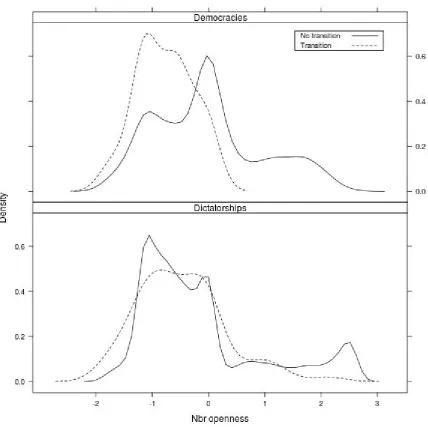
For a first look at the data, Figure 2 plots the density ofNbr Opennessfor country-years in the sample,

splitting these by their initialDemocracyscore (on the Przeworski measure) and by whether they

experi-enced a transition, i.e. a change in theDemocracyscore. For democracies, in particular, countries which

experienced a transition clearly had less open neighbors. The pattern for dictatorships is similar but less

striking.

[Figure 2 about here]

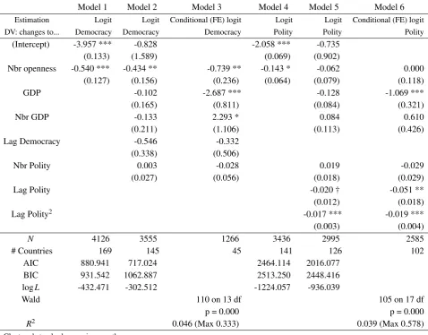
The first set of regression results is shown in Table 2. For the Democracydependent variable, the

co-efficient onNbr Opennessis consistently negative and significant, as the theory predicts. For thePolity

dependent variable, it is only significant in the bivariate specification.

[Table 2 about here]

The lack of significance in the Polity regressions could arise because changes in Polity are capturing

something other than real changes in the level of democracy (minor reforms, or measurement error by

the coders), or because the Democracy results are spurious. To investigate further, these regressions

were rerun twice, with alterations to the dependent variable: (1) only counting a change in the level

of democracy if the Polity score moved by 3 or more points and (2) only counting a change if Polity

moved by 3 or more points, andthe head of state was removed by irregular means, according to the

Archigos dataset of political leaders (Goemans, Gleditsch and Chiozza, 2009). Using only large changes

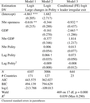
does not affect the significance ofNbr Openness.20However, as Table 3 shows,when only large changes

combined with irregular removal of the head of state are counted, the results change: the coefficient on

Nbr Opennessbecomes much larger, and is significant in the fixed effects specification. This suggests

that the weak results from thePolityregressions are due to consensual reforms that result in small changes

to the Polity score, and/or to subjective coding decisions.

[Table 3 about here]

It is unlikely that changes to the level of democracy arise similarly in democracies and dictatorships, and

it is clearly of interest whether asset mobility has the same effect in each case. To investigate this, I run

a dynamic logit model, allowing the effects of the independent variables to vary depending on whether

the country is a democracy. Thus, the estimations become:

log

pit

1−pit

= α+β1Democracyi,t−1+β2NbrOpennessi,t−1...t−5+β3NbrOpennessi,t−1...t−5Democracyi,t−1+εit

log

pit

1−pit

= α+β1Democracyi,t−1+β2NbrOpennessi,t−1...t−5+β3NbrOpennessi,t−1...t−5Democracyi,t−1

+Controlsit−→γ +ControlsitDemocracyi,t−1

− →

δ +εit.

log

pit

1−pit

= αi+β1Democracyi,t−1+β2NbrOpennessi,t−1...t−5+β3NbrOpennessi,t−1...t−5Democracyi,t−1

+Controlsit−→γ +ControlsitDemocracyi,t−1

− →

δ +εit.

[Table 4 about here]

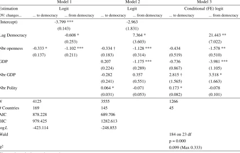
Results are shown in Table 4.21 In each model, the first column shows the effect of the independent

variables on the odds of a dictatorship becoming a democracy, and the second column shows their effect

on the odds of a democracy becoming a dictatorship. The table clarifies the effect ofNbr Openness. As

the theory predicts, this is negative for both kinds of transitions. However, the coefficient on dictatorships

is much smaller in size, and becomes insignificant in the fixed effects specification. Thus, democracies

appear to be stabilized by their neighbors’ financial openness, while the evidence that the same holds

true for dictatorships is weaker.

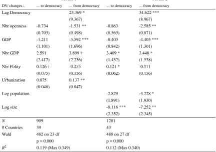
To check the robustness of this result, I reran the dynamic logit including some further independent

variables which are often supposed to affect the probability of transitions. Table 5 shows the results.

Model 1 includes a variable for urbanization. Model 2 includes population and country size. The effects

of Nbr Openness do not change significantly in either model. In further robustness checks, I varied

the sample, by including OECD countries and by excluding Soviet countries. Again, results are not

substantively different.22

21_{Dynamic fixed effects logit models suffer from bias if the initial value of the dependent variable is correlated with the fixed} effects (this is the “initial conditions problem”). To avoid this, I also ran a random effects model controlling for per-country averages of the IVs, as in Wooldridge (2005). Results were substantively similar to the fixed effects estimations. Also, the fixed effects model is very similar to a model in which the dependent variable is the logged odds of countryibeing a democracy at timet, rather than the logged odds of a transition at timet. (The two models are not identical, since the country fixed effects have different interpretations.) Again, running this model gives substantively the same results.

[Table 5 about here]

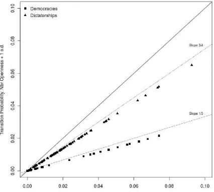
Lastly, to show the substantive size of the results, Figure 3 plots the predicted probabilities of a transition

for each of the sample countries in the year 2000, against their predicted probabilities if their value of

Nbr Opennessover the past 5 years had been one standard deviation higher.23The lines show roughly the

proportional change in probabilities: democracies would be about 1/3 as likely to experience a transition,

and dictatorships would be about 3/4 as likely.

[Figure 3 about here]

4.3 Interpretation

The cross-country evidence shows that countries were significantly less likely to experience transitions

to or from democracy when their neighbors had recently been financially open. This effect is most clear

for breakdowns in democracy. Coefficients are smaller for democratic transitions, and fail to achieve

significance in the fixed effects specification. Thus, the evidence supports Hypothesis 1b, and offers

weaker support for Hypothesis 1a.

It is interesting to consider how alternative theories might explain the link between asset mobility and

changes in democracy. One theory is that economic growth leads to transitions, and that neighboring

countries’ openness to capital increases wealth in a way not captured by GDP. However, Table 4 shows

that within a country, higher GDP is associated with greater democratic stability but not with

transi-tions to democracy. The same holds for neighboring countries’ openness. Thus, a mechanism affecting

democratic stability via increasing GDP cannot be ruled out, but theories in which wealth causes

democ-ratizations are not supported. Another theory claims that financial openness is associated with the spread

of democratic ideas. The control on neighbors’ Polity scores is meant to capture this effect. Table 4

shows that neighbors’ Polity scores are indeed associated with democratizations. However, there is no

evidence that neighbors’ financial openness causes democratizations: if anything, the reverse. Lastly,

financial openness might alter the industrial structure, increasing the power of the urban bourgeoisie.

Controlling for urbanization (Model 1 in Table 5) does not change the effect of financial openness, and

indeed urbanization appears to increase the likelihood of democratic breakdowns. Nevertheless, other

unobserved changes in social structure cannot be ruled out.

In short, while factor mobility’s effect on democracy is strongly supported in this data, it may work via

a different mechanism from the one proposed here. However, most extant theories predict that

global-ization should be positively associated with democratglobal-ization as well as democratic stability, while the

theory here predicts an association with stability of both democracies and dictatorships, and in this sense

is closer to what the data shows.

5

Conclusion

In the political economy literature to date, globalization has been understood as a process which benefits

some groups in society and harms others, leading to class or factor coalitions which seek to extend or

mitigate its effects, and encouraging democratization by protecting capital owners from redistributive

taxation. This leaves out an important part of the story, which is that factor mobility forces states’

rulers to compete more in providing services to those under their rule. This paper examines the political

implications, arguing that interstate competition substitutes for internal competition. When democracy

has costs as well as benefits – as may be the case in many developing countries (Bates, 2008) – increasing

external competition will alter the tradeoffs for citizens, lowering their demand for democracy so that

there is more political stability but also less democratization. When democracy has been established in

a country, the same logic lowers rulers’ incentives to attempt antidemocratic coups, since their level of

rents will be limited even in an autocracy by external competition. Overall, there is simply less to fight

over when factor mobility constrains the sovereign. The evidence shows that factor mobility is indeed

associated with fewer breakdowns in democracy, and there is some evidence that it also causes fewer

democratizations.

For political scientists, the view of globalization as heightened competition between state apparatuses

leads to further interesting research possibilities. In particular, future work could focus on integrating

redistribution and agency concerns. How do elites weigh the risks of unconstrained dictatorship against

Another development would be to analyse how and when rulers choose to increase the costs of exit, for

instance by limiting visas, imposing capital controls or policing their borders. Lastly, there are cases

where factor mobility seems linked to political pathologies. For instance, in Fiji, ethnic tensions may

have been exacerbated by the ease of exit (if it is easy to leave, it may also be easy to force others out);

while in Zimbabwe, as described in Section 3.6, the mass exodus of workers to South Africa may have

pushed rulers towards a strategy of short-term plunder. Qualitative case studies would help develop our

understanding of these more complex dynamics.

References

Acemoglu, D. and J. A Robinson. 2006. Economic origins of dictatorship and democracy. Cambridge

University Press.

Ashworth, S. and E. B. de Mesquita. 2006. “Monotone Comparative Statics for Models of Politics.”

American Journal of Political Science50(1):214–231.

Bates, R. H. 2008. When things fell apart: state failure in late-century Africa. Cambridge Univ Pr.

Bewley, T. F. 1981. “A critique of Tiebout’s theory of local public expenditures.”Econometrica: Journal

of the Econometric Societypp. 713–740.

Blonigen, B. A. 2005. “A review of the empirical literature on FDI determinants.”Atlantic Economic

Journal33(4):383–403.

Boix, C. 2003. Democracy and Redistribution. Cambridge University Press.

Charter Cities Foundation. 2009. http://www.chartercities.org/concept.

URL:http://www.chartercities.org/concept

Cheibub, J. A., J. Gandhi and J. R. Vreeland. 2009. “Democracy and dictatorship revisited.” Public

Choicepp. 1–35.

Chinn, M. D. and H. Ito. 2008. “A new measure of financial openness.”Journal of Comparative Policy

Eaton, J. and M. Gersovitz. 1984. “A theory of expropriation and deviations from perfect capital

mobil-ity.”The Economic Journal94(373):16–40.

Eichengreen, B. and D. A. Leblang. 2006. “Democracy and globalization.”NBER Working Paper.

Epple, D. and A. Zelenitz. 1981. “The Implications of Competition Among Jurisdictions: Does Tiebout

Need Politics?”The Journal of Political Economy89(6):1197.

Gibbon, E. 1776. The Decline and Fall of the Roman Empire. PHOENIX ILLUSTRATED.

Gleditsch, K. S. 2002. “Expanded trade and GDP data.”Journal of Conflict Resolution46(5):712.

Goemans, H. E., K. S. Gleditsch and G. Chiozza. 2009. “Introducing Archigos: a dataset of political

leaders.”Journal of Peace research46(2):269.

Heston, A., R. Summers and B. Aten. 2006. “Penn world table version 6.2.”Center for International

Comparisons of Production, Income and Prices at the University of Pennsylvania10.

Hirschman, A. O. 1970. Exit, Voice, and Loyalty: Responses to Decline in Firms, Organizations, and

States. Harvard University Press.

Jones, B. F. and B. A. Olken. 2005. “Do Leaders Matter? National Leadership and Growth Since World

War II*.”The Quarterly Journal of Economics120(3):835–864.

Li, Q. and R. Reuveny. 2002. “Economic globalization and democracy: An empirical analysis.”British

Journal of Political Science33(01):29–54.

Marshall, M. G., K. Jaggers and T. R. Gurr. 2009. “Polity IV Project: Political regime characteristics

and transitions, 1800-2007.”University of Maryland.

Mayda, A. M. 2009. “International migration: A panel data analysis of the determinants of bilateral

flows.”Journal of Population Economicspp. 1–26.

Meldrum, Andrew. 2007. “Refugees flood from Zimbabwe.”

http://www.guardian.co.uk/world/2007/jul/01/zimbabwe.southafrica.

Olson, M. 1993. “Dictatorship, democracy, and development.”The American Political Science Review

87(3):567–576.

Olson, M. 1996. “Distinguished lecture on economics in government: big bills left on the sidewalk: why

some nations are rich, and others poor.”The Journal of Economic Perspectives10(2):3–24.

Przeworski, A., J. A Cheibub, M. E Alvarez and F. Limongi. 2000. Democracy and Development:

Political Institutions and Material Well-being in the World, 1950-1990. Cambridge University Press.

Rogowski, R. 1989. “Commerce and coalitions: How trade affects domestic political alignments.”

Princeton, NJ.

Rudra, Nita. 2005. “Globalization and the Strengthening of Democracy in the Developing World.”

Amer-ican Journal of Political Science49(4):704–730. ArticleType: primary_article / Full publication date:

Oct., 2005 / Copyright  c2005 Midwest Political Science Association.

URL:http://www.jstor.org/stable/3647692

Scotchmer, S. 2002. “Local Public Goods and Clubs.”Handbook of Public Economics4:1997–2042.

Tavares, J. and R. Wacziarg. 2001. “How democracy affects growth.” European Economic Review

45(8):1341.

Teorell, J., S. Holmberg and B. Rothstein. 2008. “The quality of government dataset.”version 15May08.

University of Gothenburg: The Quality of Government Institute, http://www. qog. pol. gu. se.

Tiebout, C. M. 1956. “A Pure Theory of Local Expenditures.” The Journal of Political Economy

64(5):416–424.

UNCTAD FDI statistics. 2009. http://stats.unctad.org/fdi.

URL:http://stats.unctad.org/fdi

Vanhanen, T. 2003. Democratization: A comparative analysis of 170 countries. Routledge.

Weidmann, Nils B., Doreen Kuse and Kristian Skrede Gleditsch. 2010. “The Geography of the

Westhoff, F. 1977. “Existence of equilibria in economies with a local public good.”Journal of Economic

Theory14(1):84–112.

Wooldridge, J. M. 2005. “Simple solutions to the initial conditions problem in dynamic, nonlinear panel

data models with unobserved heterogeneity.”Journal of Applied Econometrics20(1):39–54.

Appendix 1: Proofs

I first prove that the bad type ruler invests either ˆLor 0.

Proof. Lˆ is the interior maximizer of(1−d)(f(L)−u)−L. IfL>0 and f(L)−u≤0 then the ruler

receives −Lutility and would prefer to set L=0. Otherwise, ifL>Lˆ, then by concavity of (2), the

ruler could reduceLa little and increase his expected utility; ifL<Lˆ, then by concavity, the ruler could

increaseLand increase his utility.

Using this I prove Claim 1:

Proof. From (2), investing ˆLgives

(1−d)(f(Lˆ)−u)+−Lˆ

while investing 0 gives

(1−d)(−u)+.

Ifu≤0 then these become(1−d)(1−u+f(Lˆ))−Lˆ and(1−d)(1−u)respectively. Since(1−d)f(Lˆ)−

ˆ

L>0 by the definition of ˆLand by concavity of f, ˆLgives more utility.

Ifu>f(Lˆ)the two expressions become−Lˆ and 0 respectively; investing 0 is preferred since costly effort

will not prevent migration.

If 0<u< f(Lˆ)then the expressions are(1−d)(f(Lˆ)−u)−_Lˆ _{and 0. Rearranging gives the condition in}

Lastly I show that if (1−d)(f(Lˆ)−u)>Lˆ then u≤ f(Lˆ), and that if u≤0 (and ˆL>0) then (1−

d)(f(Lˆ)−u)>Lˆ. Therefore, the condition in the Claim covers all three cases.

If(1−d)(f(Lˆ)−u)>Lˆthenu≤f(Lˆ), since otherwise(1−d)(f(Lˆ)−u)<0≤Lˆ. Ifu≤0 and ˆL>0 then

(1−d)(f(Lˆ)−u)≥(1−d)f(Lˆ)>Lˆ. The second inequality holds because ˆLsolves f0(Lˆ) =1/(1−d)

and f is strictly concave.

I next show that LB(d,u) is decreasing in d and that there is a discontinuous jump downwards at the

crossover point from investing ˆLto investing 0.

Proof. First remember that ˆL is decreasing ind. Next, recall that zero investment occurs when ˆL≥

(1−d)[f(Lˆ)−u]. This is true whenuis high enough; it is then no longer worthwhile for the ruler to

invest. It is also true for high enoughd. To see this, differentiate the LHS of (6) with respect todto give

u−f(Lˆ).

(The effects ofdon ˆLcancel out since f0(Lˆ) =1/(1−d).) This expression increases ind. Ifu>0, when

d is high enough it will be positive, so that an increase ind increases the LHS of (6); but if so (6) must

hold in any case, since ˆL≥0≥(1−d)[f(Lˆ)−u]. For lower values ofd it becomes negative (since as

d→0, ˆL→L∗, and f(L∗)>u), and if so a further decrease ind will increase the LHS of (6) and may

make the inequality false. Also, at the crossover point, ˆL>0 unlessd=1, by definition of ˆL. (Indeed, at

d=1 (6) always holds with equality.) But if there is another crossover point, it must haved<1. Hence

ˆ

L>0 at the crossover point.

Thus, for givenu, eitherLB(d,u) =0 always, orLB(d,u) starts atL∗, decreases until the inequality holds,

at which point ˆLis positive, and thereafter is constant at 0.

Proof of Lemma 2

Proof. When the bad ruler invests positively,LB=Lˆ>0. From Claim 1 it can be seen that this holds for

an open subset of the parametersuandd. So we can setLB=Lˆ on an open subset around any givend

andu. Sinceu<f(Lˆ) = f(LB)by the conditions in Claim 1, citizen utility can be rewritten as

γf(L∗) + (1−γ)[dγf(LB(d,u)) + (1−dγ)u]

Differentiating this byd gives the expression in (5). Differentiating again byugives

∂2UCIT

∂d∂u =

−(1−γ)γ<0,

since ˆLis constant inu. The negative cross-partial suffices to show decreasing differences.

Proof of Lemma 3

Proof. From (2), the ruler’s utility can be writtenUB = (1−d)(f(Lˆ)−u)−Lˆ, since f(Lˆ)−u by the

conditions for positive investment in Claim 1. As before, this holds on an open interval around our

pa-rameters. Differentiating this first byuthen bydgives∂2UB

∂d∂u=1>0, which shows increasing differences.

To show thatUBis decreasing ind, apply the Envelope Theorem: ∂_∂U_dB =−(f(Lˆ)−u)<0.

Proof of Proposition 4

Proof. The ruler decreasesd(by the maximum amount∆, since his utility is decreasing ind) if

UB(d−∆)−c≥UB(d),

and this defines a cutpoint

¯

c=UB(d−∆)−UB(d) =−

Z d d−∆

∂UB

below which the ruler changesd. The condition in the Proposition, combined with the previous Lemmas,

shows that ∂2UB

∂d∂u>0 for alld∈[d−∆,d+∆]. Therefore, an increase (decrease) inudecreases (increases)

¯

c. Since the distribution of costs has full support onR+, the probability thatc≤c¯is strictly less (more)

ifuincreases (decreases).

The argument for the citizens is almost identical and is omitted.24

Variable Definition Source

Polity POLITY2 score Polity IV 2008 dataset

(Marshall, Jaggers and Gurr, 2009)

Note: Periods of anarchy (-77 in POLITY1) were coded as missing

Democracy Democracy score Cheibub, Gandhi and Vreeland

(2009)

Financial openness KAOPEN score Chinn and Ito (2008)

GDP Real GDP per capita Gleditsch (2002) via QOG

dataset (Teorell, Holmberg and Rothstein, 2008)

Head of state irregular exit Archigos dataset (Goemans,

Gleditsch and Chiozza, 2009)

Distances cshapes dataset (Weidmann,

Kuse and Gleditsch, 2010)

Urbanization % population urban Vanhanen (2003) via QOG

dataset (Teorell, Holmberg and Rothstein, 2008)

Population Penn World Tables (Heston,

Summers and Aten, 2006)

Country size cshapes dataset (Weidmann,

Kuse and Gleditsch, 2010)

Model 1 Model 2 Model 3 Model 4 Model 5 Model 6

Estimation Logit Logit Conditional (FE) logit Logit Logit Conditional (FE) logit

DV: changes to... Democracy Democracy Democracy Polity Polity Polity

(Intercept) -3.957 *** -0.828 -2.058 *** -0.735

(0.133) (1.589) (0.069) (0.902)

Nbr openness -0.540 *** -0.434 ** -0.739 ** -0.143 * -0.062 0.000

(0.127) (0.156) (0.236) (0.064) (0.079) (0.118)

GDP -0.102 -2.687 *** -0.128 -1.069 ***

(0.165) (0.811) (0.084) (0.321)

Nbr GDP -0.133 2.293 * 0.084 0.610

(0.211) (1.106) (0.113) (0.426)

Lag Democracy -0.546 -0.332

(0.338) (0.506)

Nbr Polity 0.003 -0.028 0.019 -0.029

(0.027) (0.056) (0.018) (0.029)

Lag Polity -0.020 † -0.051 **

(0.012) (0.018)

Lag Polity2 -0.017 *** -0.019 ***

(0.003) (0.004)

N 4126 3555 1266 3436 2995 2585

# Countries 169 145 45 141 126 102

AIC 880.941 717.024 2464.114 2016.077

BIC 931.542 1062.887 2513.250 2448.416

logL -432.471 -302.512 -1224.057 -936.039

Wald 110 on 13 df 105 on 17 df

p = 0.000 p = 0.000

R2 0.046 (Max 0.333) 0.039 (Max 0.578)

Clustered standard errors in parentheses

†_{significant atp< .10;}∗_{p< .05;}∗∗_{p< .01;}∗∗∗_{p< .001}

Omitted: splines of time since last change to/from democracy (or increase/decrease in Polity), five-year dummies

Model 1 Model 2 Model 3

Estimation Logit Logit Conditional (FE) logit

DV Large changes in Polity + leader irregular exit

(Intercept) -4.863 *** 1.682

(0.205) (2.717)

Nbr openness -0.616 ** -0.344 -0.932 *

(0.215) (0.288) (0.437)

GDP -0.161 -2.663 *

(0.270) (1.286)

Nbr GDP -0.377 1.814

(0.346) (1.217)

Nbr Polity 0.006 0.013

(0.054) (0.077)

Lag Polity 0.066 † 0.073

(0.035) (0.050)

Lag Polity2 -0.009 -0.008

(0.008) (0.012)

N 4107 3006 644

# Countries 171 127 23

AIC 443.575 362.027

BIC 494.139 794.629

logL -213.788 -109.013

Wald 469 on 17 df, p = 0.000

R2 0.039 (Max 0.290)

Clustered standard errors in parentheses

†_{significant atp< .10;}∗_{p< .05;}∗∗_{p< .01;}∗∗∗_{p< .001}

Omitted: splines of time since last shift to/from democracy, five-year dummies

Model 1 Model 2 Model 3

Estimation Logit Logit Conditional (FE) logit

DV: changes... ... to democracy ... from democracy ... to democracy ... from democracy ... to democracy ... from democracy

(Intercept) -3.799 *** -2.963

(0.143) (1.831)

Lag Democracy -0.608 * 7.364 * 21.443 **

(0.253) (3.603) (7.022)

Nbr openness -0.333 * -1.102 *** -0.334 † -1.128 *** -0.434 -1.578 **

(0.137) (0.211) (0.183) (0.314) (0.519) (0.510)

GDP 0.207 -1.175 *** -0.736 -3.981 ***

(0.224) (0.289) (0.867) (1.105)

Nbr GDP -0.282 0.357 2.815 † 3.518 *

(0.241) (0.551) (1.565) (1.663)

Nbr Polity 0.064 * -0.071 0.173 * -0.078

(0.031) (0.053) (0.082) (0.101)

N 4125 3555 1266

# Countries 169 145 45

AIC 878.228 689.706

BIC 979.425 1282.613

logL -423.114 -248.853

Wald 184 on 23 df

p = 0.000

R2 0.099 (Max 0.333)

Clustered standard errors in parentheses

†_{significant atp< .10;}∗_{p< .05;}∗∗_{p< .01;}∗∗∗_{p< .001}

Omitted: splines of time since last shift to/from democracy, five-year dummies

For Model 3, the estimation with cubic splines did not converge; quadratic splines were used instead

Model 1 Model 2 DV: changes... ... to democracy ... from democracy ... to democracy ... from democracy

Lag Democracy 23.369 * 34.622 ***

(9.367) (8.967)

Nbr openness -0.734 -1.531 ** -0.863 -2.585 **

(0.703) (0.498) (0.563) (0.871)

GDP -1.211 -5.592 *** -0.403 -4.403 ***

(1.101) (1.696) (0.842) (1.301)

Nbr GDP 2.591 3.899 † 3.409 * 3.448 *

(2.417) (2.236) (1.452) (1.538)

Nbr Polity 0.126 † -0.255 0.121 * -0.171

(0.075) (0.156) (0.062) (0.156)

Urbanization 0.075 0.137 ** (0.048) (0.047)

Log population -2.829 -4.228 *

(1.891) (1.930)

Log size -8.116 *** -7.252 **

(2.352) (2.345)

N 909 1201

# Countries 39 43

Wald 482 on 23 df 488 on 27 df

p = 0.000 p = 0.000

R2 0.119 (Max 0.349) 0.112 (Max 0.340)

Clustered standard errors in parentheses

†_{significant atp< .10;}∗_{p< .05;}∗∗_{p< .01;}∗∗∗_{p< .001}

Omitted: splines of time since last shift to/from democracy, five-year dummies, continent/decade dummies (model 3).