University of Warwick institutional repository:
http://go.warwick.ac.uk/wrap
A Thesis Submitted for the Degree of PhD at the University of Warwick
http://go.warwick.ac.uk/wrap/59339
This thesis is made available online and is protected by original copyright.
Please scroll down to view the document itself.
Interactions in the Integer Quantum Hall Effect
by
Christoph Sohrmann
Thesis
Submitted to the University of Warwick
for the degree of
Doctor of Philosophy
Physics
Contents
List of Figures v
Acknowledgments viii
Declarations ix
Abstract xi
Abbreviations xii
Chapter 1 Introduction 1
Chapter 2 The Integer Quantum Hall Effect 7
2.1 Electrons in a Magnetic Field . . . 7
2.2 The Quantised Hall Effect . . . 9
2.3 Disorder, Scaling, and Electron-Electron Interactions in 2D . . . 14
Chapter 3 Modelling the IQHE 19
3.1 Chalker-Coddington Network and RG Approach . . . 19
3.2 Random Landau Matrix Model . . . 23
3.3 Hamiltonian Diagonalisation . . . 24
Chapter 4 Hartree-Fock Approximation 28
4.2 Solving the HF Equations with Spin . . . 35
4.3 Calculation of the Total HF Energy . . . 37
4.4 The Roothaan Algorithm . . . 38
4.5 The Level Shifting Algorithm . . . 43
4.6 The Optimal Damping Algorithm . . . 44
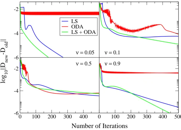
4.7 Convergence . . . 49
4.8 Further Improvements . . . 50
Chapter 5 Properties of the 2DEG 52 5.1 Density of States and Mobility . . . 52
5.2 Local Density of States . . . 56
5.3 Chemical Potential and Compressibility . . . 56
5.4 Participation Ratio . . . 58
5.5 Screening . . . 59
Chapter 6 Electronic Compressibility 64 6.1 Compressibility Patterns . . . 64
6.2 Coulomb Blockade . . . 66
6.3 Numerical Results in the(B, ne)-Plane . . . 69
6.4 Charge Density Distribution and Screening . . . 74
6.5 Breakdown of Linear Screening . . . 78
6.6 Compressibility Patterns in the FQHE . . . 83
6.7 Conclusion . . . 84
Chapter 7 Conductivity 86 7.1 Linear Response: The Kubo Formula . . . 88
7.2 Periodic Boundary Conditions, Berry Phase, and Conductivity . . . 89
Chapter 8 Interaction Effects in STS Measurements 100
8.1 Probing a 2DEG . . . 100
8.2 The Donor Potential . . . 102
8.3 The Tip Potential . . . 104
8.4 Numerical Results . . . 105
Chapter 9 Summary and Conclusion 112
Appendix A Calculation of Periodic Matrix Elements 116
Appendix B Mobility 118
Appendix C Commutators 120
Appendix D Guiding Centre Velocity 121
List of Figures
1.1 Schematic sketch of a Hall bar geometry . . . 2
1.2 Hall conductance and longitudinal resistance schematically. . . 3
1.3 Measured Hall voltage . . . 4
1.4 Compressibility measurement of Ilani et al. . . 6
2.1 Schematic sketch of theβ-function for different dimensions. . . 16
2.2 Transition from a Wigner electron lattice to a Wigner hole lattice. . . . 18
3.1 Charge density for localised and delocalised states . . . 21
3.2 Chalker-Coddington network of saddle points . . . 22
3.3 RG structure for Chalker-Coddington network . . . 23
4.1 Oscillatory behaviour of the Roothaan algorithm . . . 41
4.2 HF-potential for two electrons during the HF iteration . . . 42
4.3 Convergence behaviour of three algorithms. . . 50
5.1 DOS atB = 3T for non-interacting and interaction system . . . 55
5.2 Local density of states in 3D . . . 57
5.3 Scaling functions of the participation ratioPα at B= 3T . . . 60
5.4 Power-law fit of the system size dependence ofPα atB = 3 . . . 61
6.1 Measurement of the inverse electronic compressibility . . . 65
6.3 κ−1 for a HF-interacting system as a function of position and electron density . . . 70
6.4 κ−1 for a non-interacting system in the(B, n
e)-plane . . . 71
6.5 κ−1for a HF-interacting system with disorder strengthW/d2= 1.25meV
in the (B, ne)-plane . . . 72
6.6 κ−1 for a HF-interacting system with disorder strengthW/d2 = 2.5meV in the (B, ne)-plane . . . 73
6.7 κ−1for a HF-interacting system with disorder strengthW/d2= 3.75meV
in the (B, ne)-plane . . . 74
6.8 Spatial distribution of non-interacting electron density atν = 1/2 . . . 75
6.9 Spatial distribution of HF-interacting electron densityν = 0.1 . . . 77
6.10 Spatial distribution of HF-interacting electron densityν = 0.9 . . . 78
6.11 Spatial distribution of Hartree-interacting electron density atν = 1/2 . 79
6.12 Spatial distribution of HF-interacting electron density at ν= 1/2 . . . . 80
6.13 Cross-sections of spatial distribution of HF-interacting electron density
atν = 0.9 . . . 81
6.14 κ−1 for HF-interacting system in the(W/d2, ne)-plane . . . 82
7.1 Measured Hall conductance in the(Vg, B)-plane . . . 87
7.2 σxy for a spinless non-interacting system with disorder strengthW/d2= 2.5meV in the (B, ne)-plane . . . 94
7.3 σxy for the lowest two spin levels of a HF-interacting system with disorder
strengthW/d2 = 2.5meV in the(B, ne)-plane . . . 95 7.4 σxy for the lowest two orbital Landau levels of a HF-interacting system
with disorder strengthW/d2 = 2.5meV in the (B, ne)-plane . . . 96
7.5 Same as Figure 7.3 but with disorder strengthW/d2 = 1.25meV and for
a different disorder configuration . . . 97
7.7 σxy for non-interacting and HF-interacting system for different disorder
strengths as a function of electron density,ne . . . 99
8.1 Tunneling in STS measurements . . . 102
8.2 Effective impurity potential atz= 0nm. . . 105
8.3 Measured and calculated LDOS for lowest four spin-split Laundau levels 106
8.4 LDOS for HF-interacting system for different tip and interaction strengths110
Acknowledgments
I am glad to finally have the opportunity to express my gratitude to a number of people.
Firstly, I am very grateful for the moral, financial, and scientific support I received
generously from my supervisor Rudolf Andreas R¨omer, and the motivation to come to
Warwick in the very first place. I am indebted to the Department of Physics for the
financial support without which I wouldn’t have made it. A big thanks also to Katsushi
Hashimoto and Markus Morgenstern for the exciting and productive collaboration as
well as numerous discussions greatly broadening my field of view. Particular gratitude
goes to Alexander Croy for countless, stimulating discussions with a lot of really bright
ideas I nicked off him. Furthermore, I wish to express my appreciation for many valuable
discussion with Nick d’Ambrumenil, Nigel Cooper, John Chalker, Bodo Huckestein, and
David Leadley. I owe credit to the Centre for Scientific Computing (especially Christine,
Matt, and Grok) for the pleasant surroundings and the UK National Grid Service for
catering for my outrageous needs for computing resources.
Outside the office, I would like to give a big credit to my mum for being so
sup-portive during the years, Yoshi and Wing for the time we lived and laughed together and
for introducing me to fields of research where¯his absurdly insignificant (ludicrous!), and
of course Kristin for curing my headaches during the final year of my PhD. Ultimately,
this list would be fairly incomplete without acknowledging important contributions by
Lavazza, Budget Gazebos Ltd., DMR, Google, the guy who invented Japanese curry,
Keith Jarrett and The Surfkings for delicious food, Linda also for delicious food, and
Declarations
I hereby declare that this thesis represents my own work and to the best of my knowledge it contains no materials previously published or written by another person, nor material which to a substantial extent has been accepted for the award of any other degree at The University of Warwick or any other educational institution, except where the acknowledgement is made in the thesis. Any contribution made to the research by others, with whom I have worked at The University of Warwick or elsewhere, is explicitly acknowledged in the thesis.
Parts of this work were and will be published in conference proceedings and peer-reviewed
journals:
(i) Compressibility in the Integer Quantum Hall Effect within Hartree-Fock
Ap-proximation, C. Sohrmann and R. A. R¨omer, phys. stat. sol. (c)3, 334-338 (2005)
(ii) Compressibility stripes for mesoscopic quantum Hall samples, C. Sohrmann
and R. A. R¨omer, New J. Phys. 9, 97 (2007)
(iii) Kubo conductivity in the IQHE regime within Hartree-Fock, C. Sohrmann
(iv) Quantum percolation in the quantum Hall regime, C. Sohrmann, J. Oswald,
and R. A. R¨omer, invited review for ”Lecture Notes in Physics” (Springer),
in preparation
(v) Interaction effects for the Integer Quantum Hall Effect, C. Sohrmann and
R. A. R¨omer, submitted to phys. stat. sol.
(vi) Real-space spectroscopy of Spin and Landau Levels in the Integer Quantum
Hall Regime, K. Hashimoto, C. Sohrmann, M. Morgenstern, J. Wiebe, R. A. R¨omer,
Abstract
This thesis captures a numerical study of the interplay between disorder and
electron-electron interactions within the integer quantum Hall effect, a regime where the
presence of a strong magnetic field and two-dimensional confinement of the electrons
profoundly affects the electronic properties. Prompted by recent novel experimental
results, we particularly emphasise the behaviour of the electronic compressibility as a
joint function of magnetic field and electron density, which appears to be insufficiently
accounted for by the widely used independent-particle model. Our treatment of the
electron-electron interactions relies on the Hartree-Fock approximation so as to achieve
system sizes comparable to the experimental situation. We find numerical evidence for
various interaction-mediated effects, such as non-linear screening, local charging, andg
-factor enhancement. Important implications for the phase diagram may arise, although
a study of the scaling of the participation ratio seems to imply a universal critical
be-haviour independent of interactions. Furthermore, we examine the Hall conductivity in
a similar fashion, which also displayed interaction-promoted features in transport
mea-surements. Our mesoscopic simulations only reproduce some of the observed features,
suggesting the presence of effects beyond numerical tractability. Finally, we model
scan-ning tunneling spectroscopy experiments and systematically investigate the influence of
the tip induced potential as well as the interactions among the electrons. Our results
show a strong dependence on the filling factor and may greatly assist the interpretation
Abbreviations
page
2DES/2DEG Two-dimensional electron system/gas 24
DOS Density of states 52
EOM Equation of motion 10
FQHE Fractional quantum Hall effect 3
HF Hartree-Fock 28
IQHE Integer quantum Hall effect 2
LDOS Local density of states 56
LL Landau level 12
LS Level-shifting algorithm 41
MIT Metal-to-insulator transition 5
MOSFET Metal-oxide-semiconductor field-effect-transistor 1
ODA Optimal damping algorithm 44
PBC Periodic boundary conditions 11
QH Quantum Hall 5
QD Quantum dot 67
RHF Restricted Hartree-Fock 34
SET Single electron transistor 64
STS Scanning tunneling spectroscopy 5
TDDOS Thermodynamic density of states 52
i Imaginary unit defined byi
2=−1 11
χn(x) Harmonic oscillator eigenfunction 12
ϕn,k(r) Landau wave function 13
Hn(x) Hermite polynomials 12
L Linear dimension of square sample 13
Nφ Number of flux quanta 13
NLL Number of Landau levels 26
Ne Number of electrons 13
ne(r) Charge density at positionr 27
ne Average charge density in the sample 8
ν Filling factor 13
n0 Landau level density 26
C Matrix of eigenvectors 30
Cα,σ Eigenvector α with spinσ 36
Dσ Spin dependent density matrix 31
∂x Derivative with respect to x 10
˙
x Time derivative ofx 10
ǫF Fermi energy 30
f(ǫ) Fermi function defined by f(ǫ) =
exp(ǫ−ǫF)/kBT+1−1 39
fα Fermi function of state α, i.e. f(ǫα) 30
µB Bohr magneton 24
g∗ effective g-factor 24
m∗ effective electron mass 10
kB Boltzmann constant 53
lc Magnetic length 12
˜
ν Critical exponent 14
ρ(E) Density of states at energy E 14
Hσ
2DES Spin dependent Hamiltonian 24
VI Electron-impurity interaction 24
VC Electron-electron interaction 24
v(q) Fourier transform of electron-electron interaction 29
H General Hamiltonian 26
He−e General electron-electron interaction Hamiltonian 26
He−bg General electron-background interaction Hamiltonian 26
Hbg−bg General background-background interaction Hamiltonian 26
H0 General one-particle Hamiltonian 26
H1 General two-particle Hamiltonian 26
γ Interaction strength 25
ζ, ξ, η Cyclotron coordinates 11
R, X, Y Guiding centre coordinates 11
ε Small parameter for numerical purposes 37
Chapter 1
Introduction
The advent of semiconducting devices and their use in integrated circuits was nothing
short of a social revolution and clearly marked the brink of a new era. Transistors
and diodes became indispensable as they made their way into pretty much all areas
of everyday life, opening up a world of instant communication and pervasive access to
information. Solid state physics can certainly be regarded as one key player in the race
for an interconnected, educated society, since technical progress especially in this field
requires a thorough and profound knowledge of the underlying microscopic phenomena.
Indeed, physics has come a long way ever since. Yet, our understanding is still far
from complete. In this work we attempt to contribute a small bit. Using numerical
methods, we focus on one particularly interesting phenomenon which triggered many
new developments in condensed matter physics. In 1980, an altogether unexpected
discovery was made by Klaus von Klitzing and coworkers [1] when carrying out Hall
measurements on a metal-oxide-semiconductor field-effect transistor (MOSFET). They
discovered that for a system of electrons confined to two dimensions and subject to a
strong, perpendicular magnetic field, B, the resistivity tensor, ρ, and the conductivity
tensor,σ, can freeze to the form
ρ=
0 h/e2i
−h/e2i 0
and σ =
0 −ie2/h ie2/h 0
Figure 1.1: Schematic sketch of a Hall bar geometry for the measurement of the lon-gitudinal and the Hall resistance. The current flows from the so-called source to the drain, indicated by the arrow on the left and on the right, respectively.
withibeing an integer. Astonishingly, it turned out that this quantisation holds over a
wide range of B or the applied voltage, forming quantised plateaus, and is completely
independent of the sample geometry and choice of material. A commonly adopted
geometry is, for instance, the Hall bar, as sketched in Figure 1.1. In between those
plateaus, the Hall conductivity,σxy, performs a transition and the longitudinal
conduc-tivity, σxx, assumes a finite value ofe2/h, as shown schematically in Figure 1.2. This
was the fruitful discovery of the integer quantum Hall effect (IQHE). Contrary to the
classically expected linear relation betweenρxy andB, this quantisation of transport sets
in at very low temperatures and high sample quality. The importance of the discovery
lies in the precision and resilience of the quantisation and allowed for a high precision
determination of the fine structure constant, defined as α = e2/(2ǫ0hc), where c is the vacuum speed of light and ǫ0 the vacuum permittivity. Ultimately, the IQHE was
adopted as a metrological standard, defining the international reference resistance as
Figure 1.2: Schematic sketch of the plateau structure of the Hall conductance as well as the finite longitudinal resistance at the plateau transitions in the IQHE.
with an absolute error of ±5·10−3Ω [2]. For the importance of this discovery von
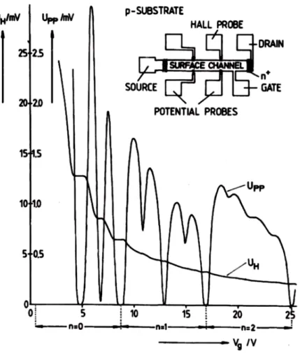
Klitzing was awarded the Nobel prize in 1985. The original measurements are depicted
in Figure 1.3. The IQHE was soon followed by another unexpected, even more surprising
finding. When carrying out Hall measurements on even cleaner samples, higher fields,
and lower temperatures, Tsui, St¨ormer, and Gossard discovered in 1982 [3] that the
Hall conductivity becomes quantised also at intermediate magnetic fields or voltages
and acquires certain fractional values ofe2/h, such as1/3,2/3,2/5, and so on. Owing to the logic, this effect was calledfractional quantum Hall effect (FQHE) and rewarded
with a Nobel prize in 1998. Whereas the IQHE was soon motivated with a gauge
argument in a non-interacting system of electrons [4], the FQHE turned out to be far
more complicated and could only be explained with correlated many-body states [5] or
collective excitations with fractional charge [6, 7], albeit still lacking a firm, microscopic
derivation. The scope of this work will be limited to the IQHE for which single-particle
models [4, 8–16] have successfully been able to reproduce general features such as the
position and height of the plateaus. However, interactions become an essential part
Figure 1.3: Measurement of the Hall voltage (UH) and longitudinal voltage (UPP) as
compressibility (see Figure 1.4) [17,18] or the conductance [19,20], enhancement of the
g-factor [21], negative compressibility [22], filling factor dependence of the Landau level
width [23], or the Hall insulator [24]. In this work we outline our numerical investigations
of such electron-electron interaction related effects using a mean-field HF-approach and
thereby neglecting higher correlations among the electrons. Since HF accounts for
Thomas-Fermi screening effects while at the same time leading to a critical exponentν˜
whose value is found to be consistent with results of non-interacting approaches [25,26],
this appears to be a reasonable starting point.
We now outline the structure of this work: In Chapter 2 we review the behaviour of electrons in the quantum Hall (QH) regime. Chapter 3gives a brief overview over some numerical methods which have been very successful in reproducing the main features of
the integer quantum Hall effect, although mostly in a single-particle picture. InChapter 4, we turn to the derivation and implementation of the HF-approximation. We discuss convergence properties of three different algorithms. InChapter 5we outline important properties of two-dimensional electron systems and compare numerical results for the
non-interacting and the HF-interacting case. We also touch the question of universality
of the metal-to-insulator transition (MIT). InChapter 6we present our numerical results on the compressibility in the(B, ne)-plane and compare the experimental findings [17,18]
with our non-interacting and HF-interacting simulations. Chapter 7 is dedicated to further experimental evidence for electron-electron interaction effects in the IQH regime
deduced from transport experiments. We derive an expression for the Hall conductivity of
a HF-interacting system and present simulation results also as a joint function ofB and
ne. In Chapter 8 we focus on scanning spectroscopy microscopy (STS) experiments,
where the influence of the scanning tip on the imaging data is unclear. We present a
systematic investigation of how the tip potential and the electron-electron interaction
Chapter 2
The Integer Quantum Hall Effect
2.1
Electrons in a Magnetic Field
The first quantitative investigations on the behaviour of electrons in a magnetic field
were carried out back in the 19th century. Edwin Hall discovered during his dissertation
in 1879 [27] that when he placed a conductor in a magnetic field with a direction
per-pendicular to the flowing current, a voltage drop could be picked up along the direction
perpendicular to both the field and the current. What must have come as a surprise
back then was the discovery of the nowadays well-known classical Hall effect and has
its origin in the Lorentz force, FL, which acts on a moving charge, −e, having velocity
v, subjected to a magnetic field,B, as follows
FL=−ev×B . (2.1)
The carriers that are deflected into the direction of this Lorentz force accumulate at
the edge of the sample and thereby create an induced electric field,EH, perpendicular
to the current and the magnetic field. This field exerts a force, FH = −eEH, on the
carriers which compensates the Lorentz force such that
Hall expected his experiments to reveal a dependence of the resistivity along the current
direction on the magnetic field, which he did not find due to the compensating Hall
field [28]. Along the direction of this Hall field a voltage, UH, could be measured
which displayed an astonishing independence of the experimental set up [29]. How
this comes about becomes clear if we relate thisHall voltage to the geometry and the
applied current as follow. We assume the magnetic field perpendicular to the current
and measure the Hall voltage in the direction of the Hall field, EH =v×B, and our
particular set-up gives |EH| = |v||B|. Now the sample can be viewed as a capacitor
which obeys |EH| = UH/W, where W is the dimension of the sample into the Hall
direction. Assuming the validity of the Drude model [29], we take the current density
to be
j=−enev, (2.3)
whereneis the carrier concentration, and the currentI =A|j|withA being the
cross-section of the sample, we finally obtain
UH=−I|B|W
eneA
=AHI|B|W
A , (2.4)
with the Hall coefficient for electrons, AH = −(ene)−1. This coefficient results from
microscopic sample properties and will thus only depend on the chosen material and
not be affected by the experimental set-up. Therefore the Hall effect can be used to
obtain information about charge transport properties such as carrier concentration or
mobility of the carriers in a material. Especially the sign of the Hall coefficient (in our
case a minus sign) can change if holes are involved in charge transport. This is used as
a way of distinguishing electron and hole transport [30]. In electronics, the Hall effect is
exploited in so-called Hall sensors which are used to determine magnetic field strengths,
angles, positions, velocities, or currents [30].
For the following considerations we lift the constraint of the experimental set-up above
and allow for an arbitrary direction of the current, which means that we have to switch
having transport in the two dimensional (x,y)-plane only. This is experimentally realised
for instance in heterostructures, cleaved semiconductor surfaces, MOSFETs, graphene,
just to name a few [31]. Now we define the tensors that link the applied field and the
resulting current. We define a resistivity tensor,ρ, and a conductivity tensor, σ, as
ρ=
ρxx ρxy ρyx ρyy
and σ=ρ−1=
σxx σxy σyx σyy
, (2.5)
whereσxy =−σyx is theHall conductivity,ρxy =−ρyx theHall resistivity,σxx =σyy
the longitudinal conductivity, andρxx =ρyythe longitudinal resistivity. The conductivity
tensors thereby describes the current response to the field,
j=σE . (2.6)
which is Ohm’s law. Hence we have as
σxx= ρxx ρ2
xx+ρ2xy
and σxy =− ρxy ρ2
xx+ρ2xy
. (2.7)
What we have discussed so far are material parameters that are not directly accessible
to measurements. The conversion from the actually measured Hall conductance, GH,
and Hall resistance, RH, involves geometric factors such as the cross-section or the
length of the sample. However, under certain circumstances, two dimensional systems
are a beautiful exception. If we apply an external field E = (Ex,0), resulting in a
current j = (jx,0), a Hall field EH = (0, EH) is induced. With UH = EHW and EH=−ρxyjx =−ρxyI/W obtained through Equation (2.6), we findUH=−ρxyI, and
thusRH=−ρxy, independent of any geometry parameters. However, one assumption which remains is that the Hall voltage has to be measured precisely on opposite sites of
the sample. In the following we will see under which circumstances even this becomes
irrelevant for the measurement.
2.2
The Quantised Hall Effect
The geometric corrections usually involved in the Hall effect can be eliminated by
becomesθH→ 90◦. In this case,σxx = 0, and no voltage drops along the sample and therefore the Hall voltage may be picked up at two arbitrary points on the edges of the
sample. Thereby making true material parameters, namely the ’-ivities’ instead of the ’-ances’, experimentally accessible. The discovery of this exceptional effect, theinteger quantum Hall effect(IQHE), by von Klitzing was awarded with the Nobel prize in 1985.
In this section we will focus on the origin of the IQHE. Therefore we first turn
back to the classical picture for a two-dimensional system with perpendicular magnetic
field B = (0,0, B). We assume the same set-up as before, where EH =RHjx. Now
plugging in the Drude current density from Equation (2.3), as well as EH = vxB, we
find for the classical Hall resistance
RH= B
ene
. (2.8)
Thus, for a fixed carrier density, in the classical picture one would expect a linear relation
between the Hall resistance and the magnetic field. It is very instructive to first study
the dynamics of the electrons purely classical before we turn to a quantum mechanical
description. Assuming the magnetic field again inz-direction, the classical equation of
motion (EOM) reads
∂2r ∂t2 =
¨ rx ¨ ry
=− e
m∗ (E+v×B) =−ωc
E B + ˙ ry
−r˙x
, (2.9)
where we have introduced the frequency ωc = eB/m∗, the meaning of which will
become clear very soon. With a fieldE= (E,0), as usual, we find the solution
r(t) = E
ωcB
cosωct
sinωct
− EB
0
t
+r0 , (2.10)
with the arbitrary constant of integration r0. As expected, Equation (2.10) describes
a cyclotron motion with angular frequencyωc, which will thus be called cyclotron fre-quency, superimposed onto a drift motion into y-direction. If the cyclotron motion is
very fast we can take a time average,
hrit= lim ∆→∞∆
−1Z ∆/2 −∆/2
and only the drift motion will remain. Thus no force is acting on the electrons on
average, i.e.¨r= 0, and we recover Equation (2.2).
Let’s now turn to a quantum mechanical description. The stability of the plateaus
strongly points to an effect due to the quantisation of the electron movement in the
magnetic field. We will neglect any edge effects and study the bulk Hamiltonian for the
2D electrons, which can be written as
h0 = 1
2m∗(p−eA) 2 = 1
2m∗π
2 , (2.12)
wherep is the momentum and Athe vector potential of the magnetic field determined
by B = ∇ ×A. We have introduced the canonical momentum π = p−eA. The choice of the vector potential will of course be irrelevant for any observable quantity,
but will make a difference to the symmetry of the eigenfunctions of the Hamiltonian.
For purposes of numerical implementation, a convenient choice should be according to
the geometry. For a square sample with periodic boundary conditions (PBC) the Landau
gauge,
A=B(0, x)T , (2.13)
appears most convenient and will be employed throughout this work. Assuming a similar
behaviour in the quantum case as we found for the classical case, we compute the EOM
as ˙ πx ˙ πy = i ¯
h[h0,π] =ωc
πy
−πx
, (2.14)
and find an equivalent expression to the classical Equation (2.9). Thus we introduce
thecyclotron coordinateζ, as well as the guiding centrecoordinates R, as
ζ =
ξ η
and R=
X Y
, (2.15)
respectively. The true electron motion can now be written asr=R+ζ .Integrating
the EOM we find
π=mωc
η
−ξ
and we can write the Hamiltonian as
h0 =
¯
hωc
2lc
ζ2 = ¯hωc 2lc
(η2+ξ2). (2.17)
Thus, the clean Hamiltonian commutes with R and therefore does not lead to a drift
motion. The wave functions describing the cyclotron motion can be found from the
Schr¨odinger equation
h0ϕ(r) =Eϕ(r) . (2.18)
In Landau gauge h0 is independent of y, thus commutes with py = −i¯h∂y which is therefore conserved. This also implies thath0 andpy have common eigenstates and
eigenvalues, which we callky. Hence for the states we immediately findϕ(r) =ξ(y)χ(x)
withξ(y) = exp[(i/¯h)kyy]. Inserting these eigenstates into the Schr¨odinger equation we find for thex-dependent part
h0χ(x) = "
− ¯h
2
2m∗ ∂2 ∂x2 −
m∗ω2 c
2
x− ky
eB 2#
χ(x) =Eχ(x) , (2.19)
This is just a 1D harmonic oscillator in a quadratic potential inx-direction around the
guiding centreX =kl2
c, where we have introduced k=ky/¯h and the magnetic length lc = p¯h/eB. The frequency of the oscillation is – just as in the classical case – the cyclotron frequency ωc. The eigenvalue of the 1D harmonic oscillator are thus the
eigenvalues of our Hamiltonian, which are given by
En= (n+ 1/2)¯hωc , (2.20)
withn= 0,1,2, . . . labeling the number of nodes, called theLandau level. Similarly we
find the eigenstates as
χn(x) = p 1
2nn!√πlc exp
−x
2
2l2 c Hn x lc , (2.21)
requirement of PBCs. In a square geometry of sizeL×L, the PBC iny-direction require exp(ikL) = 1 and therefore
k= 2π
Lj , (2.22)
withj being an integer. For the centre coordinate this means X = (2πl2c/L)j, which has to lie within the geometry, i.e. X∈(0, L]and thusj ∈[1, L2/2πlc2]. By the above considerations we found the number of states per Landau level
Nφ= L2
2πl2 c
, (2.23)
which is also the number ofmagnetic flux quanta,Φ0 =h/e, that penetrate the areaL2
at a magnetic field B, as given by Nφ=L2B/Φ0. This is probably not too surprising
since for a spin-polarised system there can be precisely one state per flux quantum in
each Landau level. In summary, the Schr¨odinger equation (2.18) with the magnetic
Hamiltonian of Equation (2.12) in Landau gauge (2.13) is obeyed by the degenerate
Landau functions [32]
ϕn,k(r) =hr|ϕn,ki=
1
p
2nn!√πl cL
exp
iky−
(x−kl2 c)2
2l2 c
Hn
x−kl2 c lc
, (2.24)
with the eigenenergies En = (n+ 1/2)¯hωc , where n labels the Landau level index
and k = 2πj/L with j = 1, . . . , Nφ the momentum. So far we have only taken into
account the periodicity iny-direction. For the torus geometry we will adapt in this work,
another modification will have to be made which we will discuss later. Now that we
have determined the number of states per Landau level, it proves very useful to define
a quantity that characterises the filling of the system, called thefilling factorν, by
ν= Ne
Nφ
, (2.25)
where Ne is the number of electrons in the system. The spectrum of h0 consists of
a sequence of δ-peaks at energies En, where each energy corresponds to an Nφ-fold
2.3
Disorder, Scaling, and Electron-Electron Interactions in
2D
In contrast, real systems will inevitably contain a certain amount of disorder due to,
for instance, impurities, imperfections, or surface contamination. Having disorder in the
system will lift the degeneracy by broadening the δ-peaked Landau levels into bands.
For a smooth disorder potential compared to the magnetic length, especially in the limit
B→ ∞, it can be shown [33] that the eigenstates will follow equipotential lines of the disorder potential at the corresponding eigenenergies and the average density of states
will then equal the overall distribution of energies in the potential, i.e. ρ(E) = P[V].
The problem of the MIT reduces to a percolation problem and it becomes clear why there
is only a single extended state in a disordered 2D energy landscape [16]. The problem
of whether a state is localised or extended can be captured with thelocalisation length,
ξ(E), a quantity which characterises the spatial spread of the wave function [33]. It has
been show [34] that at the MIT the localisation length diverges as a power,
ξ(E) =|E−Ec|−˜ν , (2.26)
whereν˜ is the critical exponent [34]. This exponent characterises the transition and is
believed to be independent of microscopic details of the impurity potential. The idea of
a percolating state has been exploited in the so-called Chalker-Coddington model [14],
which we will briefly review in one of the following sections. Up to today there exists
no perfectly conclusive theory of the MIT in the quantum Hall regime. The existence of
extended states in a 2D system was rather surprising given the fact that using a scaling
theory, Wegner [35, 36] and Abrahams et al. [37] were able to argue convincingly that
all states in 2D are localised. The effect of the magnetic field leads to a delocalisation
at a singular energy in the centre of the Landau band. This is, however, not a true
metallic phase but rather a quantum critical point that exhibits critical fluctuations
[36, 38, 39]. In absence of a rigorous mathematical description of this
have been stressed to provide quantitative results (see, e.g. , [34, 40–45]). However,
recently an perturbative formula for the localisation length for stacked 1D chains
(quasi-1D) has been given [46]. Scaling theory is a powerful tool to extract information about
localisation behaviour in disordered electronic system and gives very strong qualitative
results even with very few and straightforward assumption. The scaling approach for
disordered system is based on the idea that the conductance of a sample, g(L), solely
depends on the conductance of a smaller part of the sample, i.e. g(nL) = f(n, g(L)),
where one usually considers a hypercube in ddimensions with volume Ld [37, 47, 48]. This is called theone-parameter scaling assumption. For the analysis it is convenient to
introduce the so-calledβ-function, essentially defined as the change of the dimensionless
conductanceg with changing the sample sizeL,
β[g(L)] = L
g(L)
dg(L)
dL =
dlng(L)
dlnL , (2.27)
where the prefactor is introduced such that theβ-function becomes dimensionless.
Ob-viously, a metallic system must haveβ >0, such that the conductivity does not vanish
for L→ 0, whereas insulating behaviour will display β < 0. Contemplating a metallic system, Ohm’s law can be applied if g ≫ gc with gc ≈ π−2 [47] and the β-function
behaves to leading order asg/(e2/¯h)≈σLd−2. Thus forg→ ∞, we expectβ =d−2.
In case of an insulator, i.e.g≪gc, it seems reasonable to assume an exponential decay, g≈gcexp(−L/ξ), which yields β = ln(g/gc). Hence we find the result that in 1D the β-function is always smaller than zero and no MIT can exist. For 3D a crossing of zero
does exist and so does the MIT. The 2D case, however, is not so straightforward – even in
this simple picture. For weak disorder, a perturbative expansion ofβ in1/gas the small
parameter yieldsβ = (d−2)−c/g with a negative first order correction [49], implying that theβ-function will not cross zero. Integration of theβ-functiondg/(dlnL) =−c
yieldsg=σ−cln(L/L0), which shows a logarithmic decrease of the conductivity as the
system size increases. By the plausible assumption that the β-function is monotonic,
theβ-function can be sketched as in Figure 2.3. Scaling is of course not restricted to
Figure 2.1: Schematic sketch of theβ-function versuslngfor several spatial dimensions of the system [37]. The dotted line shows the small-gc approximation for d >2. It is
argued that the dotted line is an unlikely scenario due to the smoothness requirement.
number, or the Chern number is also common practise in obtaining information about
a system [43]. We will numerically investigate the MIT in a later chapter of this work.
The one-parameter scaling assumption implies a single exponent governing the phase
transition [50]. For the IQHE, Levine et al. [51] have show the breakdown of
one-parameter scaling. Instead, a two-one-parameter scaling arises, where both, σxx and σxy
scale with L. Finally we want to add that in the diffusive regime, delocalisation is
enhanced in the presence of a magnetic field as compared to the B = 0 case. The
reason is the suppression of weak localisation [33, 49]. Considering B = 0, the return
probability of an electron carrying out a diffusive motion in a disordered landscape is
the square of the sum of the probability amplitudes for all possible closed paths
re-turning to the starting point. Classically, all the cross terms between different loops
from time-reversed paths will not average to zero but yield a contribution due to the
constructive interference of these paths. Therefore the return probability increases in a
phase coherent system. This effect is known as weak localisation [33]. With a vector
potential present, an electron picks up a path-dependent phase along the way it travels.
A time-reversed path will have a different phase back at the starting point. With this
so-called broken time-reversal-symmetry the return probability is reduced and
delocali-sation enhanced compared to the coherent case without a vector potential. This is also
true for any dephasing process, such as inelastic scattering for instance with phonons,
photons, or other electrons. The question of how electron-electron interactions affect
the electronic properties will be the main subject of this work. Analytical methods are
sparse and usually describe a certain aspect only approximately. Numerical methods,
for instance, can treat disorder and interactions exactly. Some approximations of the
electron system are, however, still required. In our simulation, the underlying crystal
structure will be incorporated as a renormalisation of the electron mass [49] and the
interaction with crystal defects and dopants as a smooth, random disorder potential.
The ions are treated as a smooth background charge providing overall charge neutrality
for the system. Regarding the electron-electron interactions, it has been shown that
by virtue of super universality and F invariance, universality is retained even with in-teractions present [52–54]. Therefore we expect this universality to also be supported
by our numerical calculations. We will, however, put more emphasis on comparisons
to experimental data and expect to observe distinct differences between interacting and
non-interacting model, for instance due to exchange enhanced spin splitting. In Figure
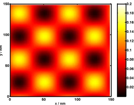
2.2 we depict the electron density of a HF-interacting system in the weak disorder limit
at half filling. Crystallisation occurs and a square lattice is formed on account of the
Figure 2.2: Spatial distribution of HF-interacting electron density for weak disorder at
Chapter 3
Modelling the IQHE
The quest for a correct and comprehensive description of IQH physics has led to a
vast number of numerical approaches and model systems. In this Chapter we want to
briefly address a few interesting methods in order to give a brief overview and to explain
some important features about IQH physics. These models have been used extensively
for investigating universality, extracting critical exponents, or conductance distributions
with high accuracy. Knowledge of the existing numerical methods is essential in choosing
the correct model for a particular problem, since each model has its advantages and
disadvantages. Methods that should be mentioned but which will not be discussed
any further are for instance tight binding lattice models [55, 56], the transfer matrix
method [57–61], the recursive Green’s function method [42], level statistics [44, 62], or
Monte Carlo [63] approaches.
3.1
Chalker-Coddington Network and RG Approach
Probably one of the most successful numerical schemes for the IQHE is the network
model introduced by Chalker and Coddington [14]. The network model is very simple and
elegant in the respect that it contains only the most necessary ingredients to describe the
mechanical tunneling and confinement. The basic form of the network model has a
completely classical interpretation. The idea to map the IQHE onto a network can
be justified most easily in the high-field limit, B → ∞, i.e. lc → 0. In this limit the cyclotron radius of the electrons vanishes and the centre coordinates take the role
of the ordinary spatial coordinates. In the following we want to briefly sketch the
justification. We assume a Hamiltonian of the form H = h0 +V(r), where V(r) is
a disorder potential due to the electron-impurity interaction. Furthermore, we assume
the eigenstates of this Hamiltonian, φα(r), are linear combinations of Landau states,
i.e. φα(r) = P
n,kCn,kα ϕn,k(r). The coefficients can be found from the Schr¨odinger
equation,H|φi=E|φi, which reads in matrix form
X n′k′
hϕnk|V|ϕn′k′iCnα′,k′ =E′αCn,kα , (3.1) and which by virtue of the form of the matrix elements,
hϕnk|V|ϕn′k′i=
Z
d2rχn x−kl2c
V(r)χn′ x−k′l2c
exp
−iy(k−k
′)
(3.2)
in matrix formP
n′k′hϕnk|V|ϕn′k′iCnα′,k′ =Eα′Cn,kα . With the high-field approximation,
the coupling between different Landau levels may be neglected and the problem can
be solved for each level individually, i.e. the n-index can be left out of the discussion.
For easier analytical treatment, the sum will be replaced by an integral, i.e. P k′ =
(L/2π)R
dk′, and the coefficient is substituted by its Taylor expansion as C(k′) =
exp[(k−k′)d/dq]C(q)|
q=k. With some algebra [16, 64] and the limit lc → 0, one can
state the problem as a differential equation. The solution yields parametrised orbits,
V(X, Y(X)) = E′ along the with equipotential lines of the disorder potential at the
respective eigenenergiesE′. In this approximation, it becomes apparent that only states
along percolating equipotential lines will be extended, which for a smooth potential is a
singular energy and thus only a single state will be extended in the limitL→ ∞ [16]. Thus, the problem of the IQHE can be mapped to a classical percolation problem [14].
In Figure 3.1 we show the charge density of a single state at the bottom and in
0 100 200 300 400 500
]
m n
[
x 0
100 200 300 400 500
]
m
n
[
y
0 100 200 300 400 500
]
m n
[
x 0
100 200 300 400 500
]
m
n
[
y
Figure 3.1: Non-interacting charge density of a single localised (left figure) and delo-calised (right figure) state for a system of sizeL= 500nm atB = 6T. States are located at aroundν = 0.1 andν = 0.5, respectively. The disorder potential is indicated by the equipotential lines.
of the disorder potential and thus the guiding centre approximation give a good account
of the situation. The difference to the classical problem of percolation is quantum
mechanical tunneling, which may allow transmission through the system away from the
classically critical point. Clearly, tunneling will occur wherever different contour lines
come very close. These points are the saddle points in the potential landscape. The
basic idea of Chalker and Coddington was to map the saddle points of the potential to a
regularly spaced network, shown in Figure 3.2, and account for tunneling by a quantum
mechanical scattering matrix at each node. A clear requirement of the model is a
smoothly varying potential according to|∇V(r)| ≪¯hωc/lc. In the original model [14],
each node has two incoming and two outgoing links. The presence of the magnetic
field requires a unique flow direction and thus imposes a certain chirality on the nodes,
depicted on the right hand side of Figure 3.2. The randomness is incorporated as a
random phase the electron acquires when being scattered at a node. This accounts
for the mapping of random distances to the regular network. One can then construct
Figure 3.2: Chalker-Coddington network of saddle points [65]. The black lines indicate equipotential lines in the disordered landscape. The red circles indicate saddle points wherever the equipotential lines come close to each other. They are modeled as scatter-ers connecting two incoming and two outgoing waves. The nodes are eventually linked up to form a network. Right: Saddle point represented as a scatterer connecting two incoming with two outgoing channels. Purple and blue circles are potential extrema.
has been successfully employed to determine the localisation length exponent, yielding
a value ofν = 2.5±0.5[14], in agreement with other methods [16]. A renormalisation scheme has moreover been introduced [44, 66], which avoids the computation of the
transfer matrix of the entire network that are replaced by a smaller ensemble of nodes,
called a super node, as depicted in Figure 3.3. This super node is then renormalised
by putting the result back into each of the nodes, thus constructing a new super node,
and the procedure is repeated until the physical quantities have converged. With this
scheme very large system sizes can be achieved conveniently using a few nodes only.
This method yields a very accurate value for the critical exponent ofν = 2.39±0.01[65]. The idea of tunneling at saddle points remains a useful concept even in the presence
of correlations among the electrons [67], and may for instance be used in an effective
φ
φ
φ
φ
2
4
1
3
II
III
V
IV
I
)
t
t
r
11 1
−r
(
1Figure 3.3: Renormalisation-group structure (super node) for the Chalker-Coddington network [65] consisting of five individual nodes. Blue nodes indicate individual scatterers. The dotted nodes are neglected such that five super nodes can be joined together. Dashed lines indicate boundary conditions.
3.2
Random Landau Matrix Model
The random Landau matrix (RLM) method may be classified as a statistical approach
to IQHE physics [34, 69]. It is based on the argument that the full amount of
under-lying microscopic information is inessential for the physics and the observed electronic
behaviour. It is argued that the phase transition associated with the IQHE is captured
by a few statistical properties of the disorder potential only, such as the correlation
func-tionhV(r)V(r′)iensemble. Then the system is sufficiently described by a matrix obeying
the correct statistics, namelyhVk1,n1;k2,n2Vk3,n3;k4,n4iensemblewith the matrix elements
Vk,n;k′,n′ = hϕk,n|V|ϕk′,n′i. In this approach the correlation between the matrix el-ements is explicitly computed, and then decomposed such that the individual matrix
to the relevant information while at the same time providing access to a whole class
of systems. For instance by introducing a parameter for the correlation length of the
potential, the RLM can be tuned smoothly from a white noise limit to a slowly varying
disorder potential [69]. The construction of the RLM can be very efficient in terms of
computational complexity. However, for the purpose of this work, where sample-specific,
microscopic properties are of importance, this method is unfortunately unsuitable due
to its purely statistical character.
3.3
Hamiltonian Diagonalisation
A diagonalisation of the complete Hamiltonian may be regarded as one of the less
effective method in terms of computational efficiency. On the other hand, very few
assumptions are needed and therefore one usually refers to such calculations as ”ab
initio” calculations. One is, however, faced with the problem of choosing a suitable basis
in which the Hamiltonian has to be represented. After calculating the matrix elements
of the Hamiltonian in these basis states, a diagonalisation is performed, in most cases
numerically. This method offers perhaps the most flexibility. In addition to universal
properties obtained by averaging over different ensemble configurations, one has direct
access to microscopic properties of the 2DES for each disorder realisation. Therefore
this method seems most natural for the purpose of modeling an experimental situation
and will be used in this work. In order to model a high-mobility heterostructure in the
QH regime, we again consider a 2DES in the (x, y)-plane subject to a perpendicular
magnetic field B = Bez. A single electron in such a system can be described by a
Hamiltonian of the form
H2DESσ =hσ+VC =
(p−eA)2 2m∗ +
σg∗µ BB
2 +VI(r) +VC(r,r
′) , (3.3)
whereσ =±1is a spin degree of freedom,VIis a smooth random potential modeling the
effect of the electron-impurity interaction,VCrepresents the electron-electron interaction
term andm∗,g∗, andµ
respectively. In order to avoid edge effects we impose a torus geometry of sizeL×L
onto the system [70]. The electron-impurity interaction is modeled by an electrostatic
potential due to a remote impurity density separated from the plane of the 2DES by
a spacer-layer of thicknessd, as found for instance in modulation-doped GaAs-GaAlAs
heterojunctions [71, 72]. Within the plane of the 2DES, this creates a random, spatially
correlated potential with a typical length scaled. We useNIGaussian-type ”impurities”,
randomly distributed atrs, with random strengthsws∈[−W, W], and a fixed widthd,
such thatVI(r) =PNIs=1 ws/πd2
exp[−(r−rs)2/d2] =PqVI(q) exp(iq·r) with
VI(q) = NI X s=1
ws L2 exp
−d
2|q|2
4 −iq·rs
, (3.4)
where qx,y = 2πj/L and j = −Nφ,−Nφ−1, . . . , Nφ. The areal density of
impu-rities therefore is given by nI = NI/L2. The limit d → 0 yields a potential of δ
-type that would be more adequate for modeling low-mobility structures [31, 73]. The
electron-electron interaction potential has the form VC(r,r′) = γe2/4πǫǫ0|r−r′| =
P
qVC(q) exp [iq·(r−r
′)],with
VC(q) = e2
4πǫǫ0lc γ Nφ|q|lc
. (3.5)
The parameterγ will allow to continually adjust the interaction strength; γ = 1
corre-sponds to the bare Coulomb interaction. Choosing the vector potential in Landau gauge,
A=Bxey, the kinetic part of the Hamiltonian is diagonal in the Landau functions [32]
of Equation (2.24), as we derived earlier in Section 2.2. These functions are extended
andL-periodic iny-direction and localised in x direction. In the following chapter we
discuss the treatment of the electron-electron interaction in detail. For completeness we
now briefly focus on the single particle basis states suitable for diagonalising the
Hamil-tonian. The system’s many-body state, |Φi, is assumed to be an anti-symmetrised product of single particle wave-functionsψσα(r) (Slater determinant) [74, 75], which we choose as a linear combination of Landau states
ψασ(r) =
NLL−1 X n=0
Nφ−1 X k=0
withNLL being the number of Landau levels and the periodic Landau functions
χn,k(r) = ∞
X j=−∞
ϕn,k+jL/l2
c(r), (3.7)
in order to meet the boundary conditions. The number of flux quanta piercing the
2DES of sizeL×Lis given byNφ=L2/2πl2c, yielding a total number of M =NLLNφ
states per spin direction. The filling of the system is characterised by the filling factor
ν = Ne/Nφ, with Ne being the number of electrons in the system and areal density ne=Ne/L2. The total Landau level density is given byn0=eB/h. One problem arises,
however, when using the bare Coulomb term of Equation 3.5. The Fourier transform
describes an infinitely replicated system whose interaction energy tends to infinity [76].
This effect is condensed in the q= 0 term which leads to a divergence and has to be
handled with care [77]. We can make some progress by investigating the interaction of
the 2DEG with the background. The Hamiltonian is split into a one and a two-electron
part as follows,
H=H0+H1 . (3.8)
The two-electron part can be further decomposed as
H1 =He−e+He−bg+Hbg−bg , (3.9)
where the electron-background, and the background-background interaction. For the
Hartree case this interaction Hamiltonian can be written as
H1=
1 2
Z Z
d2rd2r′
ne(r)ne(r′)
|r−r′| + 2
ne(r)nbg(r′)
|r−r′| +
nbg(r)nbg(r′)
|r−r′|
(3.10)
= 1 2
X q
Assuming a homogeneous background charge distribution,nbg(r) =−eNe/L2, with the
Fourier transformnbg(q) =−e2Ne/L2δq,0, the Hamiltonian becomes
H1 =
1 2
X q
v(q)
ne(q)ne(−q)−2ne(q) eNe
L2 δq,0+ e2Ne2
L4 δq,0
(3.12)
= 1 2
X q
v(q)
ne(q)ne(−q)− e2N2
e L4 δq,0
(3.13)
= 1 2
X
q6=0
v(q)ne(q)ne(−q). (3.14)
Thus, for a system of interacting electrons the interaction with and among the
neutralis-ing background charge exactly cancels the divergentq= 0term, which is a consequence
of the Fourier transform that replicates the unit cell infinitely. In conclusion, unless
Chapter 4
Hartree-Fock Approximation
In the following we will introduce the theory of Hartree-Fock (HF) [78], which is an
effective one-particle mean-field approximation to the full many-body problem. In order
to treat interacting electron systems on the mesoscopic or even macroscopic scale,
an approximation to the immensely time-consuming many-body problem is imperative.
Hartree-Fock theory provides such an approximation which allows for reasonable system
sizes and at the same time giving a good quantitative account of most effects due to
the interactions [79–82]. The theory has been reviewed as well as refined as early as
1951 by Roothaan in the article [78]. Up to today HF theory is successfully employed to
numerous problems in solid state physics or quantum chemistry [75,83]. In this Chapter
we will derive the HF-equations adapted to our system, and discuss the questions of
convergence and efficient computation.
4.1
Derivation of the HF Equations
There exist several ways of deriving the HF equation. A very neat and appealing approach
is based on a hierarchical construction of the reduced density matrices of the full
many-body problem [84–87]. We will, however, describe the variational approach which is more
Hamiltonian for the electron-electron interactionV(r,r′)in terms of the field operators,
ˆ
ψ†(r) =X
α
ψα∗(r)ˆaα†, and ψˆ(r) =X
α
ψα(r)ˆaα , (4.1)
where ˆa†α and aˆα creates and annihilates an electron in state α, respectively. The
interaction Hamiltonian which reads
He−e=
1 2
Z Z
d2rd2r′ψˆ†(r) ˆψ†(r′)V(r,r′) ˆψ(r′) ˆψ(r) (4.2)
can thus be rewritten as
He−e= 1 2
X αβϑδ
Fαβϑδˆa†αˆaϑ†ˆaδˆaβ , (4.3)
where we have introduced
Fαβϑδ = Z Z
d2rd2r′ψ∗α(r)ψ∗ϑ(r′)V(r,r′)ψδ(r′)ψβ(r) . (4.4)
Assuming translational invariance of the interaction, as for the Coulomb interaction,
i.e.V(r,r′) =V(r−r′), we can insert the Fourier transform
V(r−r′) =X
q
v(q)eiq(r−r ′)
, (4.5)
and we get
Fαβϑδ = X
q
v(q)hψα|e
iqr
|ψβihψϑ|e−
iqr
|ψδi . (4.6)
In the case of Coulomb interactions,v(q) is given as
v(q) =
Z d2r
L2V(r−r ′)e−iqr
= c
Nφ|q|lc
, with c= e
2
4πǫǫ0lc
. (4.7)
So far we still have a full many-body problem where the number of possible states with
Ne electrons is NNφe
. This means 205
= 15504 many-body states for 5 electrons in a
system with 20 flux quanta. Thus, it is evident that an approximation is needed. For
size of the basis toNφ. We write the many-body state|Φi as a Slater determinant, an
anti-symmetrised product of single particle states,
|Φi=
ǫη≤ǫF Y
η
ˆ
a†η|0i, (4.8)
where|0i is the vacuum, and ǫF the Fermi level. Next, we find those wave functions, ψα(r), which are a minimiser of the total energy in the ground state. This energy is
given as
hΦ|He−e|Φi=hHi=
1 2
X αβϑδ
Fαβϑδhˆa†αˆa†ϑaˆδˆaβi (4.9)
= 1 2
X αβϑδ
Fαβϑδfαfϑ(δαβδϑδ−δαδδβϑ) (4.10)
= 1 2
X αϑ
fαfϑ(Fααϑϑ−Fαϑϑα). (4.11)
where δαβ is the Kronecker delta and fα is the Fermi function. In the following we
will chose a basis in which we expand the eigenstates. The clean Hamiltonian without
interactions is diagonal in the Landau functions |ϕn,ai of (2.24) and we choose the
ansatz of linear combinations of Landau states,
|ψαi= NLL−1
X n=0
Nφ X a=1
Cαn,a|ϕn,ai and hψα|=
NLL−1 X n=0
Nφ X a=1
Cαn,a∗hϕn,a| (4.12)
where the normalisation condition implies the unitarity of the matrixC, i.e.
NLL−1 X n=0
Nφ X a=1
Cαn,a∗Cβn,a=δα,β. (4.13)
Using the expansion we find for the ground state energy
hHe−ei=
1 2
X αϑ
X n,m,n′,m′
X k,l,k′,l′
fαfϑCαn,k∗Cαn′,k′Cϑ
∗ m,lCϑm′,l′
Gm,l;mn,k;n′′,k,l′′−G
m,l;n′,k′
n,k;m′,l′
(4.14)
where
Gm,l;mn,k;n′′,k,l′′ =
X q
v(q)hϕn,k|eiqr
|ϕn′,k′ihϕm,l|e− iqr
The basic idea of HF is now to find expansion coefficients which minimise the total
energy. By applying the variational principle, we can find an eigenvalue equation to
determine the matrix C. Thereby the orthonormality, i.e. P
nC∗µnCµn = 1has to be
taken care of as a constraint in the optimisation procedure. For the sake of clarity we
will omit the Landau level indices in the further derivation and use the Latin indices as
double-indices to indicate both momentum and level index. The variational equation
now reads
X µm
δ δCµm
"
hHe−ei −λµ X
n
Cµn∗Cµn−1
!#
δCµm = 0. (4.16) The coefficients and their complex conjugates can thereby be treated as independent
variables, which follows from the independence of the real and imaginary parts. Therefore
we focus on one of the two,
X µm " 1 2 X αϑ
fαfϑ X abcd
Cαa ∗Cϑc ∗
δµαδmbCϑd+δµϑδmdCαb Gc;da;b−G c;b a;d
−λµCµm∗ #
δCµm= 0 . (4.17)
The complex conjugate is derived in the same way. The two terms in the first bracket
are equal and by summing overϑanddwe get
X µm " X α fα X abc
Cαa ∗CαbCµc ∗
Gc;ma;b −Gc;ba;m−λµCµm∗ #
δCµm = 0, (4.18) which can only hold if the terms in angular brackets vanish identically. From here
onwards we will not use double-indices anymore and write out the Landau level explicitly.
Introducing the density matrix
Dn,a;m,b = X
α
fαCαn,aCαm,b∗ (4.19)
we find the HF equations which determine the matrix Coptimally with respect to the
total ground state energy as
X n′,k′
X l′,m′,l,m
Dσm,l;m′ ′,l′
Gm,l;mn,k;n′′,k,l′′−G
m,l;n′,k′
n,k;m′,l′
Cµn′,k∗′ =λµC
µ∗
This equation is a self-consistent eigenvalue equation for determiningC, which thus has
to be solved iteratively until convergence. However, the problem of constructing the
matrix according to this equation is the memory requirement as well as the complexity.
The complexity of constructing G is O(NLLNφ4) or O(NLLL8) in terms of the system
size, which is rather impractical if Nφ becomes much bigger than 100. Therefore we
have to simplify the evaluation of G, which can be done using the knowledge of the
basis functions as follows. The Landau states are again given by Equation 2.24. For
simplicity we will work in magnetic units from here onwards, i.e. lc = 1. Thus, any
length is given in units of lc and any momentum in l−c1. The matrix elements of the plane waves hence read
hϕn,i|exp(iq·r)|ϕm,ji=
1
L√2n+mn!m!π× Z
d2rexp
iq·r+i(kj −ki)y− 1
2(x−ki)
2−1
2(x−kj)
2
Hn(x−ki)Hm(x−kj).
(4.21)
After carrying out the Fourier transform iny-direction and substitution ofx=z+K+
whereK±= (ki±kj)/2 we find
hϕn,i|exp(iq·r)|ϕm,ji=
1
√
2n+mn!m!πδ ′
qy,2K−exp
−K−2 +iqxK+−
q2 x 4 × (4.22) Z ∞ −∞ dzexp " −
z−iqx 2
2#
Hn(z−K−)Hm(z+K−)
(4.23)
where the δ′-function is a periodic Kronecker delta function as given in Appendix E.
With the substitutionx=z+iqx/2this yields a standard integral (see Formula 7.377 in [89]) that can be solved analytically. After some manipulation we find form≤n
hϕn,i|exp(iq·r)|ϕm,ji=δ
′ qy,ki−kj
r
2nm!
2mn!exp
−q
2
4 + i
2qx(ki+kj)
× (4.24)
iqx−qy 2
n−m Lnm−m
q2
2
and for m > n,
hϕn,i|exp(iq·r)|ϕm,ji=δ
′ qy,ki−kj
r
2mn!
2nm!exp
−q
2
4 + i
2qx(ki+kj)
× (4.26)
iqx+qy 2
m−n Lmn−n
q2
2
, (4.27)
whereLa
n(x) is the generalised Laguerre polynomial. Now we can simplify the
compu-tation of the spinlessFock matrix,F, which reads as
Fn,k;n′,k′ =
X l,m,l′,m′
Gm,l;mn,k;n′′,k,l′′−G
m,l;n′,k′
n,k;m′,l′
Dm′,l′;m,l , (4.28)
where the first term (Hartree term) corresponds to the classical Coulomb repulsion and
the second (Fock term) to the quantum mechanical exchange interaction, the only other
two-particle correlation effect. Using Equation (4.25) we can introduce
MKn,n′,m,m′(qy) =X
qx
v(q)
r
2nn′! 2n′
n!
r
2mm′! 2m′
m!exp
−q 2 2 + i 2qxK ×
iqx−qy 2
n−n′
−iqx+qy 2
m−m′ Lnn−′ n′
q2
2
Lmm−′ m′
q2
2
(4.29)
where due to the exponential decay we can restrict the sum over qx as q2
x<max[0,−2 ln(ǫ)−qy], with an accuracy ǫ. Now we can write the Hartree term as X
l,m,l′,m′
Gm,l;mn,k;n′′,k,l′′Dm′,l′;m,l (4.30)
= X
l,m,l′,m′
Dm′,l′;m,l
X qy
δq′y,k−k′δq′y,l′−lMn,n ′,m,m′
k+k′−l−l′(qy) (4.31)
= X
l,m,m′
Dm′,l+k−k′;m,lMn,n
′,m,m′
2(k′−l) (k−k
′) , (4.32)
and the exchange term as
− X
l,m,l′,m′
Gm,l;nn,k;m′′,l,k′′Dm′,l′;m,l (4.33)
=− X
l,m,m′
Dm′,l+k−k′;m,lMn,m
′,m,n′
2(k−k′) (k−l
![Figure 1.4: Compressibility patterns found by Ilani et al. [17] in SET measurements on high-mobility samples](https://thumb-us.123doks.com/thumbv2/123dok_us/9764238.477421/21.918.248.716.299.709/figure-compressibility-patterns-ilani-set-measurements-mobility-samples.webp)
![Figure 3.2: Chalker-Coddington network of saddle points [65]. The black lines indicate equipotential lines in the disordered landscape](https://thumb-us.123doks.com/thumbv2/123dok_us/9764238.477421/37.918.260.705.109.366/figure-chalker-coddington-network-indicate-equipotential-disordered-landscape.webp)
![Figure 3.3: Renormalisation-group structure (super node) for the Chalker-Coddington network [65] consisting of five individual nodes](https://thumb-us.123doks.com/thumbv2/123dok_us/9764238.477421/38.918.277.695.121.480/figure-renormalisation-structure-chalker-coddington-network-consisting-individual.webp)