warwick.ac.uk/lib-publications
Original citation:
Zhou, Zhemin, Luhmann, Nina, Alikhan, Nabil-Fareed , Quince, Christopher and Achtman,
Mark (2017) Accurate reconstruction of microbial strains using representative reference
genomes. Working Paper. BioRxiv: Cold Spring Harbour.
Permanent WRAP URL:
http://wrap.warwick.ac.uk/96030
Copyright and reuse:
The Warwick Research Archive Portal (WRAP) makes this work of researchers of the
University of Warwick available open access under the following conditions.
This article is made available under the Creative Commons Attribution-NonCommercial 4.0
(CC BY-NC 4.0) license and may be reused according to the conditions of the license. For
more details see: http://creativecommons.org/licenses/by-nc/4.0/
A note on versions:
The version presented in WRAP is the published version, or, version of record, and may be
cited as it appears here.
Accurate Reconstruction of Microbial Strains from Metagenomic
1
Sequencing Using Representative Reference Genomes
2
Zhemin Zhou, Nina Luhmann, Nabil-Fareed Alikhan, Christopher Quince, and Mark Achtman 3
Warwick Medical School, University of Warwick, Coventry, United Kingdom
4
Abstract. Exploring the genetic diversity of microbes within the environment through metagenomic
5
sequencing first requires classifying these reads into taxonomic groups. Current methods compare these
6
sequencing data with existing biased and limited reference databases. Several recent evaluation studies
7
demonstrate that current methods either lack sufficient sensitivity for species-level assignments or suffer
8
from false positives, overestimating the number of species in the metagenome. Both are especially
prob-9
lematic for the identification of low-abundance microbial species, e. g. detecting pathogens in ancient
10
metagenomic samples. We present a new method, SPARSE, which improves taxonomic assignments
11
of metagenomic reads. SPARSE balances existing biased reference databases by grouping reference
12
genomes into similarity-based hierarchical clusters, implemented as an efficient incremental data
struc-13
ture. SPARSE assigns reads to these clusters using a probabilistic model, which specifically penalizes
14
non-specific mappings of reads from unknown sources and hence reduces false-positive assignments.
15
Our evaluation on simulated datasets from two recent evaluation studies demonstrated the improved
16
precision of SPARSE in comparison to other methods for species-level classification. In a third
simula-17
tion, our method successfully differentiated multiple co-existingEscherichia colistrains from the same
18
sample. In real archaeological datasets, SPARSE identified ancient pathogens with≤0.02% abundance,
19
consistent with published findings that required additional sequencing data. In these datasets, other
20
methods either missed targeted pathogens or reported non-existent ones.
21
SPARSE and all evaluation scripts are available athttps://github.com/zheminzhou/SPARSE.
22
1
Introduction
23
Shotgun metagenomics generates DNA sequences directly from environmental samples, revealing uncultur-24
able organisms in the community as well as those that can be isolated. The resulting data represents a pool 25
of all species within a sample, thus raising the problem of identifying individual microbial species and their 26
relative abundance within these samples. Methods for such taxonomic assignment are either based on de
27
novo assembly of the metagenomic reads, or take advantage of comparisons to existing reference genomes. 28
Here we concentrate on the latter strategy, which relies on the diversity of genomes in ever-growing reference 29
databases. This strategy has been instrumental in identifying many causative agents of ancient pandemics in 30
reads obtained from archaeological samples by detecting genetic signatures of modern human pathogens [26]. 31
Published methods for taxonomic assignment can be divided into two categories. Taxonomic profilers
32
maintain a small set of curated genomic markers, which can be universal (e. g. used in MIDAS [16]) or clade-33
specific (e. g. used in MetaPhlan2 [24]). Metagenomic reads that align onto these genomic markers are used to 34
extrapolate the taxonomic composition of the whole sample. These tools are usually computationally efficient 35
with good precision. However, they also tend to show reduced resolution for species-level assignment [23], 36
especially when a species has a low abundance in the sample and, hence, may have few reads mapping to a 37
restricted set of markers. 38
Alternatively,taxonomic binners compare metagenomic reads against reference genomes to achieve read-39
level taxonomic classification. The comparisons can be kmer-based (e. g. Kraken [25] and One Codex [15]) 40
or alignment-based (MEGAN [6], MALT [5] and Sigma [1]). Binning methods based on kmers are usually 41
fast, whilst alignment-based methods have greater sensitivity to distinguish the best match across similar 42
database sequences. Benefiting from much larger databases in comparison to genomic markers used by 43
they also tend to accumulate inaccurate assignments (false positives) [23] due to the incompleteness of the 45
databases, resulting in reads from unrepresented taxa being erroneously attributed to multiple relatives. 46
While microbial species of low abundance are hard to identify by marker-based taxonomic profilers, the 47
estimations of taxonomic binners can be hard to interpret due to their low precision. This problem especially 48
limits their application to thein silicoscreening of microbial content in sequenced archaeological materials [8]. 49
Given that the ancient DNA fragments are expected to exist in low proportions in these samples, methods 50
need to identify weak endogenous signatures hidden within a complex background that is governed by modern 51
(environmental) contamination. Furthermore, reads from archaeological samples are fragmented and have 52
many nucleotide mis-incorporations due to postmortem DNA damage. 53
We identify two challenges that limit the performance of species-level assignments. First and foremost, 54
the reference database used for all taxonomic binnings are not comprehensive. The vast majority of microbial 55
genetic diversity reflect uncultured organisms, which have only rarely been sequenced and analyzed. Even 56
for the bacteria that have genomic sequences, their data are biased towards pathogens over environmental 57
species. This leads to the next challenge where, due to the lack of proper references, reads from unknown 58
sources can accidentally map onto distantly related references, mainly in two scenarios: 1) Foreign reads 59
originating from a mobile element can non-specifically map to an identical or similar mobile element in a 60
known reference. 2) Reads originated from Ultra-Conserved Elements (UCEs), which preserve their nucleotide 61
sequences between species, can also non-specifically map to the same UCE in an existing genome. 62
Addressing both of these challenges, we designed SPARSE (StrainPrediction andAnalysis usingR epre-63
sentative SEquences). In SPARSE, we index all genomes in large reference databases such as RefSeq into 64
hierarchical clusters based on different sequence identity thresholds. A representative database that chooses 65
one sequence for each cluster is then compiled to facilitate a fast but sensitive analysis of metagenomic 66
samples with modest computational resources. Details are given in Section 2. Further, SPARSE implements 67
a probabilistic model for sampling reads from a metagenomic sample, which extends the model described in 68
Sigma [1] by weighting each read with its probability to stem from a genome not included in the reference 69
database, hence considered as an unknown source. Details are given in Section 3. 70
We evaluate SPARSE on three simulated datasets published previously [14, 21, 23]. Comparing SPARSE 71
to several other taxonomic binning software in these simulations shows its improved precision and sensitivity 72
for assignments on the species-level or even strain-level. We further evaluate SPARSE on three ancient 73
metagenomic datasets, demonstrating the application of SPARSE for ancient pathogen screening. For all 74
three datasets, SPARSE is able to correctly identify small amounts of ancient pathogens in the metagenomic 75
samples that have subsequently been confirmed by additional sequencing in the respective studies. 76
2
Database indexing
77
2.1 Background
78
Average nucleotide identity. To catalog strain-level genomic variations within an evolutionary context, we 79
need to reconcile all the references in a database into comprehensive classifications. Since its first publication, 80
the average nucleotide identity (ANI) in the conserved regions of genomes has been widely used for such a 81
purpose [10]. In particular, 95−96% ANI roughly corresponds to a 70% DNA-DNA hybridization value, 82
which has been used for∼50 years as the definition for prokaryotic species. 83
Marakeby et al. [13] proposed a hierarchical clustering of individual genomes based on multiple levels of 84
ANIs. Extending from the 95% ANI species cut-off, it allows the classification of further taxonomic levels from 85
superkingdoms to clones. However, the standard ANI computation adopts BLASTn [2] to align conserved 86
regions between genomes, which is intractable to catalog large databases of reference genomes. We therefore 87
rely on an approximation of the ANI by MASH [18] to speed-up comparisons. 88
ANI approximation. MASH uses the MinHash dimensionality-reduction technique to reduce large genomes 89
into compressed sketches. A sketch is based on a hash function applied to a kmer representation of a genome, 90
sketch. Comparing the sketches of two genomes, MASH defines a distance measure under a simple Poisson 92
process of random site mutation that approximates ANI values as shown in [18]. 93
Parameter estimation. Ondov et al. [18] already used MASH to group all genomes in RefSeq into ANI 95% 94
clusters. We adopted slightly different parameters and extended it to an incremental, hierarchical clustering 95
system. The accuracy of the MASH distance approximation is determined by both the kmer length k and 96
the sketch size s. Increasing k can reduce the random collisions in the comparison but also increase the 97
uncertainty of the approximation. We can determinekaccording to equation (2) in [18]: 98
k=dlog|Σ|(n(1−q)/q)e,
where Σ is the set of all four possible nucleotides {A, C, G, T}, n is the total number of nucleotides and 99
q is the allowed probability of a random kmer to be found in a dataset. Given n= 1 terabase-pairs (Tbp; 100
current size of RefSeq) andq= 0.05, which allows a 5% chance for a random k-mer to be present in a 1 Tbp 101
database, we obtain a desired kmer size k= 23. Increasing the sketch size s will improve the accuracy of 102
the approximation, but will also increase the run time linearly. We choses = 4000 such that for 99.9% of 103
comparisons that have a MASH distance of 0.05, the actual ANI values fall between 94.5−95.5%. 104
2.2 SPARSE reference database
105
We combine the hierarchical clustering of several ANI levels with the MASH distance computation to generate 106
a representation of the current RefSeq [17] database. The construction of the SPARSE reference database is 107
parallelized and incremental, thus the database can be easily updated with new genomes without a complete 108
reconstruction. 109
Hierarchical clustering. In order to cluster genomes in different levels, we defined 8 different ANI values 110
L = [0.9,0.95,0.98,0.99,0.995,0.998,0.999,0.9995], in which the genetic distances of two sequential levels 111
differ by ∼ 2 fold. The first four ANI levels differentiate strains of different species, or major populations 112
within a species. The latter four levels give fine-grained resolutions for intra-species genetic diversities, which 113
can be used to construct clade-specific databases for specific bacteria. 114
The SPARSE databaseD(S, L, K) is extended incrementally as shown in Algorithm 1, withS listing the 115
sketches of all genomes already in the database andK being a hash containing the cluster assignments at 116
each levell∈Lfor each keys∈S. A new genome is integrated by finding another genome in the database 117
with the lowest distance using MASH, and clustering it with its nearest neighboursndepending on the ANI. 118
Algorithm 1Incremental SPARSE database clustering
Input: SPARSE databaseD(S, L, K), list of new genomesG
Output: Extended SPARSE databaseD0(S, L, K) 1: for eachgenomeg∈Gdo
2: sg=M ashSketch(g)
3: sn=argmins∈SM ashDistance(sg, s)
4: for0≤i≤ |L| −1]do
5: if L[i]≤1−M ashDistance(sg, sn)then
6: PushK[sn][i] toK[sg]
7: else
8: Push|S|toK[sg]
9: Pushsg toS
In the SPARSE implementation, we parallelized the database construction by inserting batches of genomes 119
at once and parallelizing sketch and distance computation, thereby scaling to the complexity of the problem. 120
the insertion order of genomes can influence the database structure. Here we utilize prior knowledge from the 122
community, so the SPARSE database is initialized first with allgold standard complete genomes in RefSeq, 123
followed by representative and curated genomes. With this strategy, the whole RefSeq database with 101,680 124
genomes (Aug. 2017) can be downloaded and assigned into ANI levels in∼ 23hrs, using 20 processes on a 125
standalone server. Further insertion of 1,000 new genomes (∼5MB) into an already established database 126
takes∼15mins. 127
Representative database. To avoid mapping metagenomic reads to redundant genomes within the database, 128
we construct a database of genome representatives for read assignment, similar to [9]. The representative 129
database consists of the first genome from each cluster defined by ANI 99% and is indexed using bowtie2-130
build [11] with standard parameters. SPARSE indexes 20,850 bacterial representative genomes in∼4 hours 131
using 20 computer processes. Representative databases of other ANI levels or clade-specific databases can also 132
be built by altering the parameters. Furthermore, traditional read mapping tools such as bowtie2 [11] show 133
reduced sensitivity for divergent reads. This is not a problem for many bacterial species, especially bacterial 134
pathogens, because these organisms have been selectively sequenced. However, fewer reference genomes are 135
available for environmental bacteria and eukarya. In order to map reads from such sources to their distantly 136
related references, SPARSE also provides an option to use MALT [5], which is slower than bowtie2 and needs 137
extensive computing memory, but can efficiently align reads onto references with<90% similarity. 138
3
Metagenomic read sampling
139
Given read mappings to the representative databases as input, we adapt a probabilistic model reconstructing 140
the process of sampling reads from a metagenomic sample to assign reads onto reference genomes. We extend 141
the model implemented in Sigma [1] by also considering that reads aligned to a genome in the reference 142
database could still be originating from an unknown source, thus avoiding to overestimate the number of 143
genomes present in the sample. We introduce a weighting for each read reflecting the probability to be 144
sampled from an unknown genome, and show in Section 4 how this improves the precision of taxonomic 145
assignments. 146
Let E denote the set of both known and potentially unknown genomes in a metagenomic sample, and 147
the set of reference genomes included in the SPARSE database is a subset G ∈ E. Let P r(ri|E) be the 148
probability of sampling a random readri from any possible source, we have 149
P r(ri |E) =P r(ri, G|E)P r(ri|G).
We denotewi =P r(ri, G|E) as the sampling probability, indicating the probability thatri is sampled from 150
any known reference genome inG. On the other hand,P r(ri|G) is the probability of generatingri givenG 151
and can be further separated as 152
P r(ri |G) =
X gj∈G
P r(ri|gj)P r(gj |G),
where P r(gj|G) is the probability that a genomegj ∈Gwas chosen to generate the read, and P r(ri|gj) is 153
the probability of obtaining readri from gj. As in Sigma, given a uniform mismatch probability σ= 0.05, 154
P r(ri|gj) can be directly calculated from the alignment of ri to genomegi with xmismatches, and can be 155
stored in a matrixQ, such that 156
Qi,j=P r(ri|gj) =σx(1−σ)l−x,
where l is the length of readri. We next describe how the sampling probability wi is inferred, by giving a 157
weight to each read that indicates the probability of being sampled from a known reference genome. Reads 158
with a low weight do not influence the optimization process used to infer the optimalP r(gj|G) for a complete 159
3.1 SPARSE sampling probability
161
We model two scenarios that can lead to non-specific mappings of foreign reads. 162
1) Since there is no systematic way of masking all mobile elements in a reference sequence, we evaluate the 163
probability of a read being drawn from the core genome. We assume that highly conserved regions are part 164
of the core genome, which has been vertically inherited, whereas variable regions likely represent horizontal 165
gene transfers (HGTs). We denote thisHGT probability as mi. 166
2) We evaluate the probability of a read originating from an Ultra-Conserved Element (UCE), by com-167
paring the read depths of the aligned genome fragments with other regions in the genome. UCEs are so 168
highly conserved that additional reads from divergent genomes are likely to map on to them, which results 169
in a higher read depth than other regions. We denote thisUCE probability as ni. Combining both cases as 170
a joint probability, we infer a weightwi for each read as 171
wi=mini.
HGT probability. Given any clustertin ANI level kthat consists ofureferences, a readri can be assigned 172
to either the core genomegc or accessory genomega of this cluster. Given the number of references v ⊆u 173
the read aligns to, we can formulate the probability of the read originating from the core genome as 174
P rt(gc|ri) =
P rt(ri|gc)P r(gc)
P r(ri)
= P rt(ri|gc)P r(gc)
P rt(ri|gc)P r(gc) +P rt(ri|ga)(1−P r(gc))
,
P rt(ri|gc) =pvc(1−pc)u−v, P rt(ri|ga) =pva(1−pa)u−v
(1)
where P r(gc) is the prior probability of any read originating from a core genomic region, and pc and pa 175
are the respective probabilities for core genomic fragments or accessory genomic fragments. Default prior 176
probabilities in SPARSE are given in Table 1. Furthermore, a read can align to multiple clusters in the same 177
ANI level k, so we average the probabilities of all such clusters for each read weighted by Q inferred from 178
the read alignment: 179
P rk(gc|ri) =
P
tmaxgj∈tQi,jP rt(gc|ri) P
tmaxgj∈tQi,j .
Finally, we consider three different ANI levels for the core genome analysis (by default 90%, 95% and 98%), 180
assigning a lower value formi if the read does not map to the core genome at any of these ANI levels: 181
mi= 1−
Y k
1−P rk(gc|ri)
. (2)
Default values for the prior probabilities were inferred from a published study of core genes across multiple 182
bacterial species [3]. We account for 1% of random deletions of core genes, which givespc = 0.99. We also 183
observed that<10% of all genes are core genes in bacterial species represented by many genomes. This results 184
in P
P r(gc) <0.1 over all three ANI levels. We arbitrarily assigned a higherP r(gc) for levels with lower 185
ANI, because a sequence fragment is less likely to be part of a mobile element if it is coincidently present in 186
more divergent genomes. Finally,∼40% of the genes in a random genome are core genes. This givesmi≈0.6 187
whenv= 1 andu= 1, which can be used to find empirical values ofpa via equations 1 and 2. 188
UCE probability. In order to compare the read coverage of each fragment in a reference genomegj with other 189
fragments of the same genome, we split its sequence into k consecutive fragments fj,k using two uniform 190
arbitrary lengths, 487 bps and 2000 bps. Here 487 is used because it is a prime, such that the ends of 191
two fragments overlap only once per Mbp. Then the read depth in each fragment, dk, follows a Poisson 192
Table 1: Default prior probabilities for three ANI levels, values inferred from [3].
ANIP r(gc) pc pa
90% 0.05 0.99 0.1 95% 0.02 0.99 0.2 98% 0.01 0.99 0.5
f(k, λ). Because of the complexity of the read alignments, we relax the probability of read depth in each 194
fragment such that a wide range of read depths retain high probabilities: 195
P r(ri|fj,k) =
f(dk,λ/ √
2)
f(λ/√2,λ/√2) fordk< λ/
√ 2,
1 forλ/√2≤dk≤ √
2λ,
f(dk, √
2λ)
f(√2λ,√2λ) for √
2λ < dk,
Since a read can again align to multiple genomesgj, we compute the UCE probability of a read as a weighted 196
average of all its alignments. If a read aligns multiple times to the same genome gj with equal alignment 197
score, we choose one fragment randomly. The UCE probability is then defined as 198
ni=
P
j(Qi,jP r(ri|fj,k)) P
jQi,j
.
Thus a lower value of ni is the result from a deviation of the general coverage at the read position in 199
comparison to the average coverage in the genome, indicating that the read is likely mapping to an ultra-200
conserved region in the genome. 201
3.2 Optimization problem
202
Knowing the weight wi for all reads ri in a whole metagenomic read set R, the task is then simplified to 203
finding optimalP r(gj|G) values that maximize the probability of the whole read set: 204
maxP r(R|E) = max Y ri∈R
P r(ri|E) = max Y ri∈R
wi
X gj∈G
Qi,jP r(gj|G)
.
The optimization problem can be solved by a non-linear programing (NLP) method. In SPARSE, we rely 205
on a modified version of the function provided in Sigma [1]. 206
After optimizing P r(gj|G), we finally assign a read to a potential reference by checking the following 207
ratio of the computed probabilities: 208
P(ri, gj) =
P r(ri, gj|G)
P r(ri, G)
=P Qi,j∗P r(gj|G) gj∈GQi,j∗P r(gj|G)
. (3)
We may assign a read to multiple references, as long as P(ri,gj)
maxgP(ri,g) ≥0.1. This allows a better abundance
209
estimation for multiple strains from the same species, in which case a read cannot be assigned unambiguously 210
to a single reference. 211
Further, let ri ∈ B ⊂ R be all reads assigned to gj. For a read ri of length l with x mismatches in 212
the alignment to its assigned reference, we have a nucleotide similarity ofsi,j= l−lx. The weighted average 213
¯
sB,j =
P ri∈B
si,jwiP(ri, gj)
P ri∈B
wiP(ri, gj)
.
Potentially, reads assigned to a single reference could still originate from several co-existing genomes, 215
with varying degrees of diversity, in the metagenome. We can identify reads from more divergent sources 216
by comparing si,j to their average similarity. If all reads assigned to a single reference originate from the 217
same genome in the metagenome, we assume that the similarity of most reads complies with the average 218
similarity over all reads. However, reads originating from very conserved regions show higher similarity than 219
the average and provide a sampling bias. On the other hand, reads originating from different more divergent 220
genomes, will show lower similarity which can be used to avoid overestimating the abundance of each cluster. 221
Therefore we compute the expected average nucleotide identitys0 forri as 222
s0i,j= min (si,j, sB,j).
This similarity reflects the ANI between each read and the assigned reference and, as described in the next 223
section, can be used to compute the abundance of each cluster in the metagenomic sample. 224
3.3 ANI cluster abundances
225
The equation miniP(ri, gj) describes the probability, for each read ri ∈ R, to be drawn from a region in 226
reference gj that is part of the core genome (mi) and has even read depth in comparison to the whole 227
chromosome (ni). In summary for all reads assigned to gj, Pimini∗P(ri, gj) gives the frequency of reads 228
originating from the core genome of gj. However, the desired read abundance for a reference gj needs to 229
also include reads from the accessory genome. Such reads have been previously suppressed when computing 230
mi. If we assume that all species have the same proportion of core genome, the relative abundances of their 231
core genomes will be equal to the relative abundance of their whole genomes. However, since this is not the 232
case [3], we need to normalize eachmi computed previously. GivenP(ri, gj) from Equation 3, for any ANI 233
90% clustert, we normalizemi for a readri as 234
m0i=
P gj∈t
P rk∈R, s0k,j≥0.9
P(rk, gj)
P gj∈t
P rk∈R,
s0k,j≥0.9
mkP(rk, gj)
∗mi.
Finally, we assign reads into clusters of all ANI levels according to the references contained in the cluster. For 235
each cluster, we only assign reads if its similarity complies with the ANI levellof the cluster, i. e.s0i, j≥l. 236
Thus the abundance of a cluster tl is computed as the sum of all read abundances assigned to all 237
genomes in the cluster weighted by their probability to originate from an unknown genome. Therefore 238
clusters containing only reads with smallni andmi probabilities will receive a low abundance value even if 239
many reads are assigned to it. 240
atl=
X gj∈tl
X ri∈R s0i,j≥l
m0iniP(ri, gj)
3.4 Taxonomic labels for ANI clusters
241
We finally assign standard taxonomic designations to all clusters at all ANI levels, in order to interpret their 242
biological meaning. Here we rely on a majority vote of all genomes in a cluster. However, the taxonomic 243
levels are restricted to certain ANI levels. For example, species are distinguished at the ANI 95% level, and 244
a species designation is therefore inappropriate for an ANI 90% cluster. Similarly, the taxonomic label for 245
4
Evaluation
247
4.1 Representative Database
248
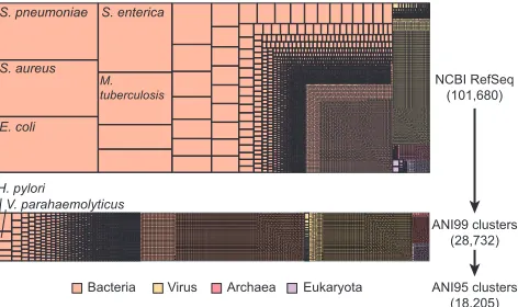
We ran SPARSE to index the RefSeq database that consists of 101,680 complete or draft genomes into 249
28,732 clusters at ANI 99% level, which were further grouped into 18,205 clusters at 95% ANI level, as 250
shown in Fig. 1. Grouping all the genomes according to their species, the resulting representative database 251
is much more evenly distributed, with a Pielou’s evenness [19] ofJ0 = 0.9, comparing toJ0 = 0.51 for the 252
whole RefSeq database. Over-representation of pathogenic organisms in the RefSeq database are largely due 253
to repeated sequencing of nearly identical genomes rather than sequencing of intra-species genetic diversities. 254
In particular, nearly half of the genomes in RefSeq are from the top 10 most sequenced bacterial species, 255
which are all human pathogens. All these genomes were grouped into 615 clusters at ANI 99% level, which 256
gives a 65-fold reduction of the data indexed for these species. 257
Bacteria Virus Archaea Eukaryota
H. pylori
V. parahaemolyticus
NCBI RefSeq (101,680)
ANI99 clusters (28,732)
ANI95 clusters (18,205) S. pneumoniae
S. aureus
S. enterica
E. coli
[image:9.612.189.425.244.384.2]M. tuberculosis
Fig. 1: Hierarchical clustering of 101,680 genomes in NCBI RefSeq database (Aug. 2017) into 18,205 ANI 95% clusters using SPARSE. Each rectangle represents such a cluster at ANI 95% level, with its area relative to the total number of genomes (top) or clusters at ANI 99% (bottom).
4.2 Simulated Data
258
We ran SPARSE on three recent simulated datasets (Sczyrba et al. [23], McIntyre et al. [14] and Quince 259
et al. [21]). For a fair comparison, the analyses for all datasets were based on a database built from NCBI 260
RefSeq and taxonomy databases dated 22th June, 2015, which is the deadline for the comparison in [23] and 261
also pre-dates the other two comparisons. We evaluated the performance of SPARSE as described in the 262
respective papers for the read-level taxonomic binners, adopting their results for the compared methods. We 263
also included Sigma using the same database as SPARSE in the comparison. We calculated sensitivity and 264
precision based on the number of true-positives (TP; correctly assigned reads), false-positives (FP; incorrectly 265
assigned reads), and false-negatives (FN; unassigned reads). 266
All simulated reads in the McIntyre et al. [14] study were generated from published complete genomes. 267
This dataset is suitable for comparing the completeness of the databases, as well as the sensitivity of the 268
read mapping approaches in different tools. Both SPARSE and Sigma were run on 18 samples that have 269
read-level taxonomic labels. SPARSE binned all the samples in 10 hours with 20 processes. The precision 270
and sensitivity of both tools in addition to six binning tools from [14] are summarized in Figure 2A. As 271
expected, all tools reached a high precision of >97%, but differed in their sensitivity. Benefiting from the 272
representative database, SPARSE and Sigma assigned the highest numbers of reads into correct species. The 273
difference between the two methods is due to their different strategies in the modeling, where Sigma assigned 274
4Samples8 12 16
0 0.2 0.4 0.6 0.8 1
0 0.2 0.4 0.6 0.8 1
SIGMA SPARSE [2015] SPARSE [2017] SIGMA
SPARSE [2015] SPARSE [2017]
PhyloPythiaS+ BlastMegan PhyloPythiaS+ mg Kraken
taxator-tk
0 0.2 0.4 0.6 0.8 1
0 0.2 0.4 0.6 0.8 1
Precision
Sensitivity
Precision E.coli strain abundance
Predicted abundance
Sensitivity
B) Sczyrba et al. medium (4) C) Quince et al. D) Quince et al. abundances A) McIntyre et al. read-level (18)
0.5 0.6 0.8
0.7
0.9 1
0.95 0.96 0.97 0.98 0.99 1
CLARK-S CLARK BlastMegan Kraken
[image:10.612.74.540.70.192.2]LMAT NBC
Fig. 2: Performances of SPARSE in simulated published datasets. The performance of all the tools in A and B, except for SPARSE and Sigma, are obtained from the respective publications [23, 14]. SPARSE was run in parallel using two different databases. [2015] uses database built from RefSeq at 2015, whereas [2017] uses up-to-date database. A) All the simulated reads in McIntyre et al. [14] were derived from published genomes. B) The Sczyrba et al. [23] used unpublished genomes for read simulations. C+D) Strain-level identification using the mockedE. colidatasets as published in [21]. C) Left: The distance-based species tree forE. colifor 45 ANI 99% representative genomes plus the five genomes used in [21] for mocked reads. The four largest ANI 98% clusters inE. coliare highlighted with colors. Right: Each column shows one of the 16 mocked samples. The true relative abundances ofE. coli strains in samples (blue) and the relative abundances of predicted strains (red) in samples are shown as colored squares. D) Comparison of trueE. coli strain abundances versus SPARSE predictions. The dashed line indicates the linear regression of the two values, withR2= 0.9948 andp <2.2e−16.
of SPARSE using the latest RefSeq database (Aug. 2017) assigned slightly more reads into species, but does 276
not improve precision. This database consists of 20,850 representative genomes, which is>2 fold the number 277
of representatives (9,707) in RefSeq 2015. 278
The datasets in Sczyrba et al. [23] are much more challenging, because all the reads were generated 279
from sequencing of environmental isolates, many of which do not have closely related references in the 2015 280
database. Furthermore, many reads do not have a known microbial species label, because they are not similar 281
to any species in SILVA [20], which was used as the gold standard in this study. We ran both Sigma and 282
SPARSE on the medium complexity datasets, and compared the results with the other methods (see Fig. 2f 283
in [23]) for the recovery of microbial species (Fig. 2B). Using 80 processes, SPARSE ran through all four 284
datasets in∼40hours. All the taxonomic binners published in [23] obtained an average precision of<30% 285
at species level, except for taxator-tk [4] with a precision of 70% along with the lowest sensitivity (∼1.25%). 286
The performance of Sigma is comparable to other binning tools, whereas SPARSE obtained an exceptionally 287
high precision of ∼ 85% while still maintaining a sensitivity of ∼ 23%. Many incorrect taxonomic bins 288
predicted in Sigma were suppressed in SPARSE, because they have low sampling probability wi to any of 289
the existing references. Again, SPARSE was also run independently against the database built Aug. 2017. 290
We recovered 63% of the species in the CAMI median datasets, with an average precision of 97%. 291
Both benchmarks evaluate the performances of taxonomic binnings on or above species level, but give 292
no resolution in intra-species diversity. DESMAN [21] allows reference-free recovery of strain-level variations 293
based on uneven read depths of different strains across multiple samples. It has been compared with two other 294
strain-level binning methods using mock E. coli samples [21]. Applying SPARSE to the same 20 genome 295
mocks, we recovered 50/51 E. coli strains in all 16 samples without any additional strains (false positives), 296
as shown in Fig. 2C. The only strain that was not recovered by SPARSE is 2011C-3493 in the 12thsample 297
(Sample733 in [21]), which accounts for only ∼0.03% of all E. coli reads in the sample. We also obtained 298
an almost exact correspondence between the relative abundances of the strains and the predictions (Fig. 2 299
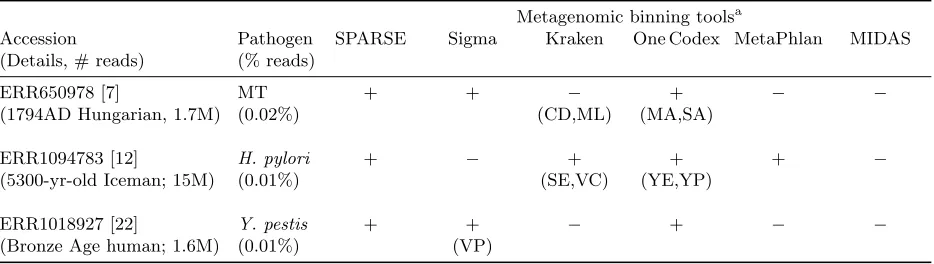
Table 2: Real archaeological datasets.
Metagenomic binning toolsa
Accession
(Details, # reads)
Pathogen (% reads)
SPARSE Sigma Kraken One Codex MetaPhlan MIDAS
ERR650978 [7]
(1794AD Hungarian, 1.7M) MT (0.02%)
+ + −
(CD,ML)
+ (MA,SA)
− −
ERR1094783 [12]
(5300-yr-old Iceman; 15M)
H. pylori (0.01%)
+ − +
(SE,VC)
+ (YE,YP)
+ −
ERR1018927 [22]
(Bronze Age human; 1.6M)
Y. pestis (0.01%)
+ +
(VP)
− + − −
a+/−for the identification of the pathogen. Abbreviations for suspicious predictions in bracket (CD:Corynebacterium
diphtheriae; MA:M. avium; ML:M. leprae; MT: M. tuberculosis; SA:Staphylococcus aureus; SE:S. enterica; VC: V. cholerae; VP:V. parahaemolyticus; YE:Y. enterocolitica; YP:Y. pseudotuberculosis).
4.3 Ancient Metagenomes
301
We further evaluated SPARSE and five additional metagenomic tools on three real sets of ancient DNA 302
reads (Mycobacterium tuberculosis from [7],Yersinia pestis from [22] andHelicobacter pylori from [12]) and 303
summarised their results in Table 2. For all samples, the presence of the targeted pathogen, although in 304
very low frequencies (≤0.02%), has been confirmed by additional sequencing in the respective publications. 305
MIDAS [16] failed in all three samples and MetaPhlan2 [24] managed to identifyH. pylori but failed in the 306
other two samples. The results for these two marker-based approaches are consistent with the simulations 307
discussed earlier. Kraken [25] and One Codex [15] are both based on kmer-based taxonomic assignment, but 308
yielded different results. Kraken only identifiedH. pylori, whereas One Codex got positive results in all three 309
samples. However both methods incurred a high number of false positives. For example, Kraken reported 310
Salmonella enterica andVibrio choleraein the Iceman sample, whereas One Codex predicted twoYersiniae. 311
All these predictions are inconsistent with results from other tools and analyses presented in the publications. 312
Sigma identified two of three pathogens but inaccurately predictedV. parahaemolyticus, which is normally 313
associated with seafood, for the human remains from the Bronze Age. SPARSE successfully identified all three 314
targeted species without any additional suspicious pathogen, which highlights its application to archaeological 315
samples. 316
5
Conclusion
317
The genetic signatures of specific microbes in metagenomic data, such as human pathogens, are often buried 318
behind the majority of reads from genetically diverse environmental organisms. This is exemplified in the 319
metagenomic sequencing of archaeological samples. Current taxonomic assignment methods compare the 320
metagenomic data with databases that do not fully capture the diversity of microbial genomes. Among these 321
tools, the marker-based taxonomic profilers fail to identify species at low abundances whereas whole genome 322
based taxonomic binners give inaccurate predictions due to non-specific read mappings on ultra-conserved 323
or horizontally transferred elements. 324
SPARSE indexes existing reference genomes into a comprehensive database with automatic hierarchical 325
clusterings of related organisms. This database is used as a reference for mapping of metagenomic reads. 326
SPARSE penalizes unreliable mappings of reads from unknown sources, and integrates all remaining into 327
a probabilistic model, in which reads were assigned to either an existing reference or unknown sources. In 328
both simulations and real archaeological data, SPARSE outperforms all existing methods, especially in the 329
precisions of species-level assignment. Furthermore, SPARSE managed to identify multiple strains of the 330
6
Acknowledgements
332
M.A., Z.Z., N.L. and N-F.A. were supported by Wellcome Trust (202792/Z/16/Z). Additional initial grant 333
support was from BBSRC (BB/L020319/1). 334
References
335
1. Ahn, T.H., Chai, J., Pan, C.: Sigma: Strain-level inference of genomes from metagenomic analysis for
biosurveil-336
lance. Bioinformatics 31(2), 170–177 (2015)
337
2. Altschul, S.F., Gish, W., Miller, W., Myers, E.W., Lipman, D.J.: Basic local alignment search tool. Journal of
338
Molecular Biology 215(3), 403–410 (1990)
339
3. Ding, W., Baumdicker, F., Neher, R.A.: panX: pan-genome analysis and exploration. bioRxiv 10.1101/072082
340
(2016)
341
4. Dr¨oge, J., Gregor, I., McHardy, A.C.: Taxator-tk: precise taxonomic assignment of metagenomes by fast
approx-342
imation of evolutionary neighborhoods. Bioinformatics 31(6), 817–824 (2014)
343
5. Herbig, A., Maixner, F., Bos, K.I., Zink, A., Krause, J., Huson, D.H.: Malt: Fast alignment and analysis of
344
metagenomic dna sequence data applied to the tyrolean iceman. bioRxiv 10.1101/050559 (2016)
345
6. Huson, D.H., Beier, S., Flade, I., G´orska, A., El-Hadidi, M., Mitra, S., Ruscheweyh, H.J., Tappu, R.: MEGAN
346
community edition-interactive exploration and analysis of large-scale microbiome sequencing data. PLoS
Com-347
putational Biology 12(6), e1004957 (2016)
348
7. Kay, G.L., Sergeant, M.J., Zhou, Z., Chan, J.Z.M., Millard, A., Quick, J., Szikossy, I., Pap, I., Spigelman,
349
M., Loman, N.J., Achtman, M., Donoghue, H.D., Pallen, M.J.: Eighteenth-century genomes show that mixed
350
infections were common at time of peak tuberculosis in Europe. Nature Communications 6, 6717 (2015)
351
8. Key, F.M., Posth, C., Krause, J., Herbig, A., Bos, K.I.: Mining metagenomic data sets for ancient DNA:
recom-352
mended protocols for authentication. Trends in Genetics 33(8), 508–520 (2017)
353
9. Kim, D., Song, L., Breitwieser, F.P., Salzberg, S.L.: Centrifuge: rapid and sensitive classification of metagenomic
354
sequences. Genome research 26(12), 1721–1729 (2016)
355
10. Konstantinidis, K.T., Tiedje, J.M.: Genomic insights that advance the species definition for prokaryotes.
Pro-356
ceedings of the National Academy of Sciences 102(7), 2567–72 (2005)
357
11. Langmead, B., Salzberg, S.L.: Fast gapped-read alignment with Bowtie 2. Nature Methods 9(4), 357–9 (2012)
358
12. Maixner, F., Krause-Kyora, B., Turaev, D., Herbig, A., Hoopmann, M.R., Hallows, J.L., Kusebauch, U., Vigl,
359
E.E., Malfertheiner, P., Megraud, F., et al.: The 5300-year-oldHelicobacter pylorigenome of the Iceman. Science
360
351(6269), 162–165 (2016)
361
13. Marakeby, H., Badr, E., Torkey, H., Song, Y., Leman, S., Monteil, C.L., Heath, L.S., Vinatzer, B.A.: A system to
362
automatically classify and name any individual genome-sequenced organism independently of current biological
363
classification and nomenclature. PLoS ONE 9(2) (2014)
364
14. McIntyre, A.B.R., Ounit, R., Afshinnekoo, E., Prill, R.J., H´enaff, E., Alexander, N., Minot, S.S., Danko, D., Foox,
365
J., Ahsanuddin, S., et al.: Comprehensive benchmarking and ensemble approaches for metagenomic classifiers.
366
Genome Biology 18(1), 182 (2017)
367
15. Minot, S.S., Krumm, N., Greenfield, N.B.: One Codex: A Sensitive and Accurate Data Platform for Genomic
368
Microbial Identification. bioRxiv 10.1101/027607 (2015)
369
16. Nayfach, S., Rodriguez-Mueller, B., Garud, N., Pollard, K.S.: An integrated metagenomics pipeline for strain
370
profiling reveals novel patterns of bacterial transmission and biogeography. Genome Research 26(11), 1612–1625
371
(2016)
372
17. O’Leary, N.A., Wright, M.W., Brister, J.R., Ciufo, S., Haddad, D., McVeigh, R., Rajput, B., Robbertse, B.,
373
Smith-White, B., Ako-Adjei, D., et al.: Reference sequence (RefSeq) database at NCBI: current status, taxonomic
374
expansion, and functional annotation. Nucleic Acids Research 44(D1), D733–D745 (2015)
375
18. Ondov, B.D., Treangen, T.J., Melsted, P., Mallonee, A.B., Bergman, N.H., Koren, S., Phillippy, A.M.: Mash: fast
376
genome and metagenome distance estimation using MinHash. Genome Biology 17(1), 132 (2016)
377
19. Pielou, E.C.: Ecological diversity. Wiley New York (1975)
378
20. Quast, C., Pruesse, E., Yilmaz, P., Gerken, J., Schweer, T., Yarza, P., Peplies, J., Gl¨ockner, F.O.: The SILVA
379
ribosomal RNA gene database project: improved data processing and web-based tools. Nucleic Acids Research
380
41(D1), D590–D596 (2012)
381
21. Quince, C., Delmont, T.O., Raguideau, S., Alneberg, J., Darling, A.E., Collins, G., Eren, A.M.: DESMAN: a new
382
tool for de novo extraction of strains from metagenomes. Genome Biology 18(1), 181 (2017)
22. Rasmussen, S., Allentoft, M.E., Nielsen, K., Orlando, L., Sikora, M., Sj¨ogren, K.G., Pedersen, A.G., Schubert,
384
M., Van Dam, A., Kapel, C.M.O., et al.: Early divergent strains ofYersinia pestis in Eurasia 5,000 years ago.
385
Cell 163(3), 571–582 (2015)
386
23. Sczyrba, A., Hofmann, P., Belmann, P., Koslicki, D., Janssen, S., Dr¨oge, J., Gregor, I., Majda, S., Fiedler, J.,
387
Dahms, E., Bremges, A., Fritz, A., Garrido-Oter, R., Jørgensen, T.S., et al.: Critical Assessment of Metagenome
388
Interpretation-a benchmark of metagenomics software. Nature Methods (2017)
389
24. Truong, D.T., Franzosa, E.A., Tickle, T.L., Scholz, M., Weingart, G., Pasolli, E., Tett, A., Huttenhower, C.,
390
Segata, N.: Metaphlan2 for enhanced metagenomic taxonomic profiling. Nature methods 12(10), 902–903 (2015)
391
25. Wood, D.E., Salzberg, S.L.: Kraken: ultrafast metagenomic sequence classification using exact alignments.
392
Genome Biology 15(3), R46 (2014)
393
26. Zhou, Z., Lundstrøm, I., Tran-Dien, A., Duchˆene, S., Alikhan, N.F., Sergeant, M.J., Langridge, G., Fotakis, A.K.,
394
Nair, S., Stenøien, H.K., et al.: Millennia of genomic stability within the invasive Para C Lineage ofSalmonella
395
enterica. bioRxiv 10.1101/105759 (2017)
![Fig. 2: Performances of SPARSE in simulated published datasets. The performance of all the tools in A and B, exceptfor SPARSE and Sigma, are obtained from the respective publications [23, 14]](https://thumb-us.123doks.com/thumbv2/123dok_us/9452387.452437/10.612.74.540.70.192/performances-simulated-published-datasets-performance-exceptfor-respective-publications.webp)