A prototype model of speculative dynamics with position based trading

WORKING PAPERS SERIES

WP07-08

A Prototype Model of Speculative

A Prototype Model of Speculative Dynamics

With Position-Based Trading

Reiner Franke

Department of Economics

University of Kiel

Kiel, Germany

December 2007

Abstract

To avoid the indeterminate and generally unbounded positions of the agents in financial market models with order-based trading, the paper considers the al-ternative of position-based strategies. To this end it extracts a prototype model from the literature, with fundamentalists, chartists, and a risk-averse market maker. The deterministic formulation of the model leads to a neutral delay-differential equation of the price, whose mathematical analysis is non-standard. The stability conditions are nevertheless quite analogous to the order-based Beja–Goldman model. The effects of parameter variations are also studied in a stochastic setting, where special emphasis is put on the misalignment between price and the time-varying fundamental value, and on the differential profits of fundamentalists and chartists.

JEL classification: C 15, D 84, G 12.

Keywords: asset pricing; fundamentalists, chartists and market maker; misalign-ment; neutral delay-differential equation; random fixed point.

Contents

1 Introduction 1

2 A direct inspiration from Beja and Goldman 3

2.1 A recapitulation of the Beja–Goldman model . . . 3

2.2 A respecification of Beja–Goldman with position-based trading . . . 6

3 The deterministic position-based prototype model 9 3.1 Formulation of the model . . . 9

3.2 Mathematical stability analysis . . . 11

3.3 Numerical investigation of the stability frontiers . . . 15

3.4 Dynamic mechanisms over a cycle . . . 21

4 A stochastic version of the model 26 4.1 Properties of a base scenario . . . 26

4.2 A stochastic equilibrium notion . . . 30

4.3 Parameter effects . . . 33

5 Conclusion 38 A Appendix 39 A.1 Proof of Proposition 3 . . . 39

A.2 Proof of Proposition 5 . . . 43

A.3 Recursive formulation of the stochastic PBT model . . . 44

A.4 Variations of parameters in the stochastic model . . . 45

1

Introduction

In theoretical financial economics it is now widely acknowledged that a paradigm shift has taken place from the representative agent with his or her rational expectations towards a behavioural approach, in which markets are populated by heterogeneous and boundedly rational agents who use rule-of-thumb strategies. The success of a new paradigm is not the least dependent on neat and catchy model designs that capture some of the key ideas under discussion and show how the basic feedback mechanisms work out. An early proto-type model of this kind has been put forward by Beja and Goldman (1980), who enthroned the market maker responsible for the gradual price adjustments together with the two archetypal groups of fundamentalists and chartists. The elementary setup and the intuitive outcome that fundamentalists tend to stabilize and chartists tend to destabilize the market had a great influence on the agent-based modelling that has begun in the 1990s. Whether the agents’ asset demand is postulated directly or derived from expected utility maximiza-tion under constant absolute risk aversion (CARA), and whether the market impact of each of the speculative groups is constant or endogenously varying over time, in many of these models the original mechanisms of the Beja–Goldman model are still shining through. In one form or another, they remain important to an understanding of what is going on in different episodes of a model-generated price history.

Not only in the Beja–Goldman model but in the vast majority of agent-based asset pricing models, the strategies of the speculative traders are expressed in terms of their orders on the market. This is a problematic feature, although it is rarely seriously discussed. At least since Markowitz (1959) it is, first, a well established standard in portfolio choice theory that investors consider holdings rather than orders as the relevant object of their profit and risk evaluation. Second and more importantly, it is also well-known that in the order-based framework the inventories of the agents and, in particular, the market maker are not anchored and so will be indeterminate. In a stochastic setting they may even easily become unbounded, which is certainly not compatible with the risk constraints of real traders.

concerned here.1 _{However, while the position-based models have examined a variety of}

single aspects so far, there is as yet no model formulation at a similar level of abstraction and insightfulness to the Beja–Goldman model. To prevent an anecdotal wilderness of bounded rationality as research proceeds further along these lines, it is the aim of the present paper to extract such a position-based prototype model from the two papers just mentioned. The outcome in the deterministic continuous-time framework will be a type of dynamic system that, as far as we know, shows up for the first time in economic modelling: a neutral delay-differential equation. It is more involved than a delay-differential equation, which is already of infinite dimension, since the right-hand side of the differential price equation contains not only the lagged level of the price but also its lagged derivative.

Despite its complexity it is possible to undertake a mathematical stability analysis. In fact, the resulting conditions on the parameters turn out to be analogous to the stability conditions in the two-dimensional Beja–Goldman model. Referring to a stylized periodic trajectory we will, however, also demonstrate that the cyclical mechanisms are different. Apart from that, a special feature of the model is an explicit risk aversion of the market maker, which has no counterpart in the order-based models.

In a second stage of the analysis, the model is reconsidered in a stochastic version, for which we employ the common assumption that the fundamental value follows a random walk. We briefly sketch the notion of a random fixed point and the pointwise convergence to it, which is a direct analogue of an attractive deterministic equilibrium. In a study of the effects of ceteris paribus variations of the model’s parameters, the qualitative notion of stability is subsequently complemented by the quantitative concept of the degree of misalignment between price and fundamental value. In addition, we investigate the impact of a change in the parameters on the long-run profits of fundamentalists and chartists, where the prospects of the latter will be generally much better than in an order-based framework. The paper proceeds as follows. In the next section we begin with a short recapitulation of the Beja–Goldman model and then try an immediate respecification of its fundamentalist

and chartist (flow) demand as position-based strategies. Since the resulting dynamics tend to be rather dull, Section 3 models the chartists in an alternative way, which, in the deter-ministic continuous-time framework, introduces lagged prices in their desired positions and thus a lagged price derivative in their market orders. This formulation yields our prototype model. The section contains the mathematical stability analysis, a numerical investigation of parameter variations and their impact on stability, and a study of the comovements of the variables on a stylized cyclical motion. Section 4 sets up the stochastic version, discusses the properties of a numerical base scenario and the random fixed point, and finally studies the effects of parameter variations. Section 5 concludes.

2

A direct inspiration from Beja and Goldman

2.1

A recapitulation of the Beja–Goldman model

Beja and Goldman (1980) distinguish three groups of participants in an asset market: two groups of speculators—fundamentalists and chartists—and a market maker. Fundamental-ists have long time horizons and base their demand on the differences between the current price and the fundamental value. Even though they might expect the gap between the two prices to widen in the immediate future, they do not trade on these short-run expectations, choosing instead to place their bets on an eventual rapprochement. Chartists, on the other hand, neglect deviations of the price from the fundamental value and concentrate on short-run changes. They use past movements of prices as indicators of market sentiments and extrapolate these into the next periods. In general, demand and supply of fundamentalists and chartists will not match the (fixed) supply of the asset. It is the primary function of the market maker to mediate transactions out of equilibrium. He executes all orders at the present price and accordingly decumulates (accumulates) inventories of the financial asset. His expectations and possible feedback effects from undesired inventories are ignored. So the demand of the market maker is treated as a residual and the only reaction considered here is the setting of a new price for the next trading round.

Goldman buy (sell) whenpis below (above)v. Chartist demand is characterized by a term

π that represents their perceptions of the current trend of prices. Both types of demand, denoted bydf _{and d}c_{, are specified in a linear manner. Introducing two positive coefficients}

φ and χ, which may be taken as indicative of the aggressiveness of fundamentalists and chartists, respectively, or of their share of wealth in total speculative capital, we have

df = φ(v−p) (1)

dc = χ π (2)

To save an extra symbol for the supply of the asset, df _{and d}c _{may be interpreted as}

excess demand (in the verbal discussion we will also economize on the expression ‘excess’). The dynamic relationships in the Beja–Goldman model are formulated in continuous time. Measuring the extent to which the market maker changes the price by a coefficientβp >0,

the evolution of prices is governed by the differential equation

˙

p = βp(df +dc) (3)

The perception π of the trend by the chartists is a predetermined variable, for which a simple adaptive updating rule is postulated. As the current ‘trend’ towards which the chartists seek to adjust their expectations is given by the instantaneous price changes, the rule is specified as

˙

π = βπ( ˙p−π) (4)

where βπ represents the speed at which these adjustments are carried out. This equation

completes the description of the Beja–Goldman model. The four equations can be reduced to two linear differential equations in the price p and the perceived trend π. They possess a unique equilibrium point p=v and π= 0, which (apart from a fluke) is either attractive or repelling. The stability condition can be formulated as follows.

Proposition 1

The equilibrium point of system (1) – (4) is asymptotically stable if χ < φ/βπ +

1/βp, and it is repelling if the inequality is reversed. A loss of stability under

ceteris paribus variations of a parameter occurs by way of a Hopf bifurcation.

˙

p = βp[φ(v−p) + χ π]

˙

π = βπ[βpφ(v−p) + (βpχ−1)π]

(BG)

The determinant of its Jacobian is unambiguously positive, which rules out saddle point instability and zero eigen-values. The trace is negative if and only if the inequality stated in the proposition is satisfied.

q.e.d

The simple condition in the proposition allows one to characterize the parameters of the model as either stabilizing or destabilizing, meaning that sufficiently high values render a possibly unstable equilibrium stable or, respectively, they turn a possibly stable equilibrium into an unstable one. In this sense, the aggressiveness of fundamentalistsφ, or their weight in the market, is a stabilizing parameter, whereas a stronger weight χof chartists is desta-bilizing. Presupposing χ>1/βp, chartists can furthermore destabilize the equilibrium by a

high adjustment speedβπ in the updating of their expectations about future price changes.

Effectively,βπ is the rate at which old price changes are discounted. Thus, for a comparison

with our main model later on, the instability feature may complementarily be also summa-rized by the statement that a short memory of chartists is destabilizing. A long memory (lowβπ), on the other hand, can always ensure stability. Finally, sufficiently sluggish price

adjustmentsβp of the market maker are stabilizing, and highly responsive adjustments are

destabilizing if βπχ>φ.

2.2

A respecification of Beja–Goldman with position-based

trad-ing

In order to cope with the problem of indeterminate, unless unbounded, inventories in the Beja–Goldman model and to reconcile this model with the literature on position-based strategies, it is straightforward to redirect its focus from, so to speak, flows to stocks. In fact, the basic idea has already been put forward in a paper by Farmer (2001), though he does not mention the relationship or analogy to Beja–Goldman and is not concerned with a deterministic skeleton of the model variants he discusses.

To begin with, let af_{, a}c_{, a}m _{be the asset positions of fundamentalists, chartists and}

the market maker. They can be positive and negative or, to be more precise, they may be conceived of as deviations from some fixed target positions. Three assumptions are then common in Farmer’s work on position-based trading, which we here formulate in continuous time. The first two are only natural for a parsimonious modelling at the macroscopic level, the third one is introduced for a more specific reason.

(1) Dividends (in case of shares) or interest from foreign bonds (in case of a foreign exchange market), as well as the receipts from an alternative riskless asset are neglected as a source of reinvestment and accumulation of wealth. In other words, the market is supposed to be closed, so that the total number of assets is conserved: every time an agent buys an asset, another agent loses it.2 _{With the interpretation as deviations from a target,}

the agents’ positions thus satisfy the following identity in every point in time,

af + ac + am = 0 (5)

(2) On the part of fundamentalists and chartists, one need not distinguish between desired and actual positions since the demand (in form of market orders) to which the desired positions give rise is always fulfilled by the market maker. As a consequence, the demand of the speculative agents and the rate of change in their positions coincide,

df = ˙af , dc = ˙ac (6)

(3) The third assumption will turn out to be a crucial mechanism to keep the market maker’s inventory within bounds and even center it around its target. The essence of the

price adjustment rule (3) is maintained, but an explicit risk aversion of the market maker is added. In Farmer’s (2001, p. 66) specification, a negative (positive) position that has been accumulated prompts him to encourage selling (buying) by raising (lowering) the price more than usual. The risk that in this way impacts on the market is measured by a coefficient

µ > 0. We also adopt Farmer’s notation and replace the coefficient βp in (3) with 1/λ,

which continues to be fixed over time. Here λ is viewed as a scale factor and is referred to as the market’s liquidity (or its depth), which nevertheless is assumed to be fixed. Upon closer scrutiny, this parameter has no time dimension and, nota bene, is not a speed of adjustment.3 _{On the whole, price changes are now described by the equation}

˙

p = (df + dc ₋ µ am)/λ (7) According to what has just been said aboutλ, the coefficientµhas the same time dimension as the left-hand side of the equation: if the underlying time unit were shortened from one day to half a day, say, then µ would have to be reduced by fifty percent, too. It is worth mentioning that a term like −µ(am _−xm_{), where x}m _{is the target level of the market}

maker’s inventory, can be part of his optimal policy in a rigorous dynamic setting which, in particular, takes his uncertainty about the future arrival of tenders into account (Bradfield, 1979).4

Having thus established a basis for dealing with position-based strategies, we can change the Beja–Goldman model’s type of demand from flows to stocks. Now fundamen-talists do notbuyif the market is undervalued but theyholdthe asset (take a long position), and if the price exceeds the fundamental value they do not sell but take a short position. Correspondingly so for the chartists if they perceive a positive or negative price trend, respectively. Formally it is postulated that the right-hand sides of eqs (1) and (2) deter-mine the desired (and realized) positions of fundamentalists and chartists (rather than their market orders),

af = κf(v−p) (8) 3_{See the derivation of the market impact function in Farmer and Joshi (2002, pp. 152f). Observe also} that in connection with the coefficient βp in eq. (3) we have avoided the expression ‘adjustment speed’ (in

contrast to Beja and Goldman, 1980, p. 237, themselves).

ac _{= κ}

cπ (9)

˙

π = βπ( ˙p−π) (10)

The last equation is eq. (4) from Beja–Goldman, which is here reproduced for convenience. The original coefficients φ and χ in (1) and (2) have been better replaced by κf and κc

in the first two equations, since they have a different dimension in the new framework. Indeed, κf and κc are viewed as being proportional to the trading capital in the hand of

the two groups of agents (cf. Farmer and Joshi, 2002, p. 158 and several times from p. 163 on). For easier erference,κf and κc are even identified with the trading capitals (which has

motivated our choice of the Greek letter).

Equations (5) – (10) constitute a linear model where the formulation of demand in Beja–Goldman has been directly translated into position-based strategies. The model is again two-dimensional with the price p and the perceived trend π as state variables. As made explicit below, its reduced-form representation can indeed do without the positions, since the market maker’s inventory in the price equation (7) is given byam _=−af_−ac _and,

using (8), (9), the latter two positions can be expressed in terms of pand π. Proposition 2 collects the results of a stability analysis of this model.

Proposition 2

System (5) – (10) is well-defined and has a unique equilibrium pointp=v,π = 0

if λ+κf #=βπκc. Under this assumption the dynamics can be characterized as

follows:

(a) The equilibrium is asymptotically stable if βπκc ≤κf.

(b) Saddle point instability prevails if βπκc >λ+κf.

(c) If κf <βπκc <λ+κf, the equilibrium is asymptotically stable if µ < µc:=

βπ(1 +αβπκc)/α(βπκc −κf), and repelling if the inequality is reversed,

where α:= 1/(λ+κf −βπκc)>0.

(d) In cases 1 and 3, the motions are monotonic (at least) if βπ ≥µ.

The model shares with the Beja–Goldman model the property that fundamentalists are sta-bilizing (a sufficiently high weight κf) and chartists are destabilizing (large trading capital

κc or fast adjustmentsβπ of their perceived trend). However, the model’s scope for cyclical

to what has been remarked on the Beja–Goldman at the end of the previous subsection, system (5) – (10) appears quite dull and not very promising for further extensions. The perhaps most interesting property is the feature stated in part (c) that a high risk aversion of the market maker could destabilize the market, though a risk aversion exceeding the critical value µc _{would be more academic than real. The phenomenon can nevertheless be}

taken as a harbinger of a theme that will become more prominent in the next sections.

Proof: Using the definition of the coefficient α in part (c) of the proposition, the two differential equations forp and π read,

˙

p = f(p,π) := α[µκf(v−p) − κc(βπ−µ)π]

˙

π = βπ[f(p,π)−π]

The determinant of the Jacobian matrixJ isαβπµκf. Hence detJ <0 and the equilibrium

is a saddle under the condition stated in the second part of the proposition. The rest of the proof supposes α >0, so that the determinant is positive. The trace of the Jacobian can be written as traceJ =₋αµ(κf −βπκc) − βπ(1 +αβπκc), which establishes part (a).

If κf −βπκc < 0, a negative trace is equivalent to the condition µ < µc in part (c). To

demonstrate the final part of the proposition, we can infer from an explicit calculation of the two eigen-values of the Jacobian that the system’s trajectories are monotonic if (traceJ)2₋

4 detJ = [αµκf+βπ+αβπκc(βπ−µ)]2−4αβπµκf is nonnegative. The suppositionβπ−µ≥0

ensures that this expression is not less than (αµκf +βπ)2 −4αβπµκf = (αµκf −βπ)2 ≥0.

q.e.d

3

The deterministic position-based prototype model

3.1

Formulation of the model

promising candidate are the trend followers that are put forward in a later paper by Farmer and Joshi (2002). These agents have a memory ofθ time units, and their desired positions are proportional to the price change observed over this horizon. In their discrete-time and stochastic framework, Farmer and Joshi (pp. 154ff) establish that this strategy has the potential of amplifying the noise in the price and of inducing oscillations at frequencies that are related to the length of the memory θ.

Regarding the market maker in this paper, Farmer and Joshi make no mentioning of his possible risk aversion. To deal with the problem that prices and fundamental values may easily drift apart, they rather assume a large number of trend followers and fundamentalists with individual trading capitals and, in addition, individual thresholds for entering and exiting a position. The numerical simulation experiments demonstrate that this strong heterogeneity can indeed achieve a cointegration of price and value (if the parameter choices take care of certain trade-off effects; see Farmer and Joshi, 2002, p. 167, fn 10). However, the very construction and purpose of this model make it meaningless to ask for a low-dimensional deterministic skeleton that could be studied on its own.

In order to design such a prototype model, we extract two central ideas from the concepts presented so far and combine them with the position-based fundamentalists from above. First, we use Farmer and Joshi’s (2002) specification of trend followers as our chartist strategy. This element should give sufficient prospects for dynamic feedback mechanisms generating oscillatory behaviour. Second, we reintroduce the risk aversion of the market maker from Farmer (2001), which by keeping his inventory within bounds should also be able to prevent persistent misalignment. Our analysis begins with the deterministic and continuous-time formulation of this model mix.

Since with the introduction of the time lag θ>0 chartists base their decisions on prices in two different moments in time, the time index can no longer be dropped. The (desired and realized) positions of fundamentalists and chartists are given by

af(t) = κf[v − p(t) ] (11)

ac(t) = κc[p(t) − p(t−θ) ] (12)

The evolution of prices continues to be governed by (7). By plugging (11), (12) into eq. (6) for the market orders, solving identity (5) for the market maker’s position am_(t),

and substituting the resulting expressions in the price equation (7), the market dynamics can be reduced to the following differential equation:

˙

p(t) = µκf[v−p(t)] + µκc[p(t)−p(t−θ)] − κcp˙(t−θ)

λ+κf −κc

(PBT)

The acronym PBT serves to indicate that the equation summarizes a model with position-based trading, the one that we will be concerned with in the rest of the paper.

Given µ > 0, the model has a unique equilibrium price p= v, which implies overall zero positions af _=ac _=am _{= 0 in that state. Note that without the market maker’s risk}

aversion, when µ = 0, the equilibrium price would be indeterminate and so would be the positions of fundamentalists and the market maker. Of course, this is the reason why prices do not track values in the simpler versions of Farmer and Joshi’s model (see, in particular, Farmer and Joshi, 2002, p. 159).

3.2

Mathematical stability analysis

The reduced form (PBT) of the price dynamics is of a remarkable type. The lagged price

Differential equations with delays are of infinite dimension. This is reflected by the fact that the initial conditions to start a trajectory require the specification, not of a vector with finitely many components, but of an entire time path of the state variable(s). The initial price path in the present model has also to be taken into account by the precise definition of stability.5 _{Thus, to be perfectly clear, consider a starting time t = 0, let p}o _{= p}o_(t)

be a differentiable function on the interval [−θ,0] that specifies the initial condition for system (PBT), and denote the corresponding solution of (PBT) as p = p(t;po_{(·)). The}

equilibrium point v is called stable if for any ε >0 there exists a number δ > 0 such that every initial time path po_{(·) with |p}o_{(t)−v| < δ for t ∈ [−θ,0] gives rise to a trajectory}

that satisfies _|p(t;po_{(·))−v| < ε for all t > 0. If in addition p(t;p}o_{(·)) → v as t → ∞,}

the equilibrium is calledasymptotically stable. Synonymously, also system (PBT) itself my be called (asymptotically) stable. It goes without saying that because everything is linear here, local stability amounts to global stability.

The dynamic properties of the system continue to be determined by the roots of the characteristic equation. However, what is true for delay differential equations is all the more true for neutral equations: rather than a polynomial the characteristic equation becomes a transcendental equation, which has a countably infinite number of roots (cf. Gandolfo, 1997, p. 551). The whole stability analysis rests on the conclusions that can be drawn for the real parts of these roots. The results that we are thus able to derive are summarized in the next proposition. Its proof is given in the appendix.

Proposition 3

Assume κc <λ+κf. Then the following holds:

(a) If κc <κf/2, system (PBT) is asymptotically stable.

(b) If κc >(λ+κf)/2, system (PBT) is unstable.

(c) A loss of stability under ceteris paribus variations of a parameter occurs by way of a Hopf bifurcation.

(d) If κf/2 <κc < (λ+κf)/2, there exists a bifurcation value θ" > 0 of the

lagθ such that (PBT) is asymptotically stable if 0<θ <θ"_{, and unstable}

monotonic manner. For values ofθ in a certain (possibly wide) neighbour-hood ofθ"_{, the motions of (PBT) are generically of a cyclical nature. Close}

to θ"_{, their period is T ≈2π/ν}" _>2θ"_{, where}

ν" := !

µ2_κ

f(2κc−κf)

(λ+κf) (λ+κf −2κc)

The stability conditions bear a close resemblance to those of Proposition 1 for the Beja– Goldman (BG) model. In particular, fundamentalists and chartists maintain their basic roles. Thus, a sufficiently large trading capitalκf of the fundamentalist trading group can

always stabilize the equilibrium, just like the corresponding parameterφin (BG). Chartists, on the other hand, destabilize the market if their trading capitalκcis large, which parameter

is analogous to the chartist aggressivenessχin (BG). As far as the responsiveness of prices is concerned, the counterpart of a high market liquidity λ in (PBT) is a high value of the reciprocal 1/βp of the price adjustment parameter in (BG), and both have a stabilizing

effect on the dynamics. A further common feature of the two models is their potential to generate cyclical motions of the price. Proposition 3(d) asserts that these cycles are essential in (PBT), in the sense that their period is at least twice as long as the memory of the chartists.

The memory of chartists in (PBT) and (BG) cannot be directly compared. In the discussion of Proposition 1 a long memory has been identified with slow adjustments of the perceived trend and so with low values of the adjustment speedβπ. With this interpretation

a long memory was stabilizing. In (PBT), a long memory is represented by a long time horizon θ, which according to Proposition 3(d) is destabilizing if κc is contained in the

intermediate interval (κf/2,(λ+κf)/2). This characterization would, however, be misleading

since longer lagsθ tend to increase the difference between the current and the lagged price

p(t−θ). If one wants to control this effect it would be more appropriate to specify eq. (12) as

ac_{(t) = ˜κ}

c[p(t) − p(t−θ) ]/θ (13)

The coefficientκc in eq. (PBT) would then read ˜κc/θ, and this expression remains no longer

fixed as θ varies. With this observation we can more specifically conclude that, with a given value of ˜κc, a sufficient increase of θ would eventually let the term ˜κc/θ fall below

would eventually exceed the threshold stated in part (b) of the proposition. Hence we obtain an additional stability result.

Proposition 4

Replace eq. (12) with eq. (13) in the PBT model. Then the equilibrium is

as-ymptotically stable if the lag θ is large enough, and unstable if it is sufficiently short.

Referring more loosely to the memory of chartists, we can now say that in both the BG model and the reformulated PBT model a long memory is stabilizing and a short memory is destabilizing.

The overall conclusion from the propositions is that (PBT) as a stylized model with position-based fundamentalist and chartist traders has very similar dynamic properties to the Beja–Goldman model with its order-based strategies. In a form that emphasizes the analogies between (PBT) and (BG), the parameter effects on the stability of the equilibrium point are succinctly summarized in Table 1. The present model should thus be a good basis for more ambitious small-scale modelling attempts within a position-based framework, from which one could expect comparable results, at least numerically, to what has been obtained in the order-based framework.

weight F weight C memory C liquidity risk aversion MM

PBT : S (κf) D (κc) S (θ) S (λ) D (µ)

BG : S (φ) D (χ) S (1/βπ) S (1/βp) — — Table 1: Parameter effects on stability in (PBT) and (BG).

Note: S (D) means that a sufficiently large increase of the parameter (de)stabilizes the equilibrium. Regarding θ, the specification of eq. (13) with a fixed value of ˜κc is assumed.

a definite characterization of the coefficient µ, too. As shown in Appendix A.2, the proof of the next proposition is almost a by-product of the proof of Proposition 3(d).

Proposition 5

Supposeκf/2<κc <(λ+κf)/2in eq. (PBT), consider two values µ1, µ2 of the

market maker’s risk aversion, and, fixing the other parameters, letθ"

1, θ"2 be the

corresponding bifurcation values of the lag θ. Then θ"

2 = µ1θ"1/ µ2.

The consequence of the proposition is immediate. Fix all parameters except µ and start from some intermediate value µ1 with associated bifurcation value θ1", for which we may

assume that it entails stability, θ < θ"

1. Then the proposition says that the bifurcation

lag θ" _=θ"_{(µ) is reduced as µ begins to rise. If µ rises far enough, the model’s lag θ will}

no longer be contained in the shrinking stability interval, θ > θ"_{(µ), and the equilibrium}

becomes unstable. Hence, under the given condition onκf,κc andλ, a higher risk aversion

of the market maker tends to be destabilizing. Recalling the destabilizing risk aversion found in Proposition 2(c) for our first position-based model, this result now turns out to be not so atypical after all.

The mechanism also works in the opposite direction. If initially µ = µ1 gives rise

to instability, θ > θ"

1, then a sufficient lowering of µ lets θ"(µ) increase above θ and so

renders the equilibrium stable. In this sense a low risk aversion of the market maker may be called stabilizing. It has, however, to be taken into account that this would also slow down the speed at which the market maker’s inventory approaches its target level. One easily finds numerical examples where convergence toward the equilibrium takes so long that classifying this system as stable would rather be misleading. In particular, already weak random perturbations would suffice to completely blur any tendency of the price to return to the fundamental value.

3.3

Numerical investigation of the stability frontiers

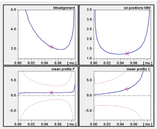
to the chartist trading capitalκc Proposition 3 tells us that such a bifurcation occurs

some-where in the interval (κf/2,(λ+κf)/2). Likewise, if 2κc >λ then a rise of κf beginning at

zero stabilizes the originally unstable dynamics somewhere in the interval (2κc−λ,2κc). A

question that the mathematical analysis could not answer, however, is whether these bifur-cations are unique, i.e., whether a reswitching of stability or instability can be ruled out. Except for the lag parameter θ, for which a unique bifurcation is ensured by Proposition 3(d), we have here to resort to numerical calculations.

Although the mathematical theory of neutral delay differential equations is quite involved, numerical bifurcations can be studied by checking a surprisingly simple criterion. To this end, letη stand for one of the parametersκf,κc,λ orµ;η is supposed to vary and

the other parameters remain fixed. Equation (21) in Appendix A.1 specifies a0, b0, b1 as

composite terms of the four coefficients, so that for the present purpose we may write them as a0 =a0(η), etc. In addition, we refer to ν" =ν"(η) from the formulation of Proposition

3. Then, consider the functional expression

h(θ,η) := a0(η) + b0(η) cos[ν"(η)θ] + b1(η)ν"(η) sin[ν"(η)θ] (14)

which is at the heart of the bifurcation analysis. From eq. (24) in the appendix and the subsequent arguments it can be inferred that an admissible value η" _{is a bifurcation value}

if, and only if, it satisfies

h(θ,η") = 0 and ν"(η")θ < π (15) Numerical studies of (15) are somewhat facilitated by the feature that, for example, λ can serve as a scaling parameter in (PBT). In fact, it is obvious that multiplyingλ as well asκf

and κc by the same factor leaves the differential equation completely unaffected. So when

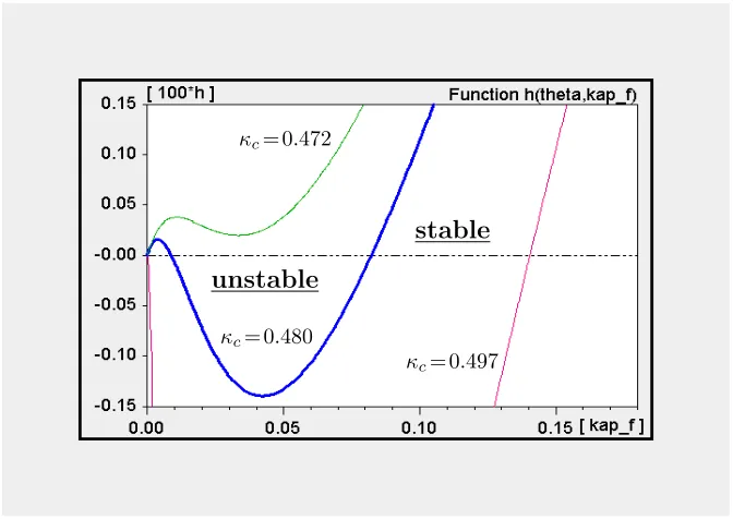
we fix the parameters in a numerical scenario, let us adopt the normalization λ= 1. An investigation of eq. (15) over a wide range of the other parameters led us to the conclusion that unique bifurcation values can be considered to be the rule. There are exceptions to this principle, but it requires some effort to find them.6 The bold (blue) line in Figure 1 presents one such counterexample for the trading capitalκf of the fundamentalists

6_{The functionη}

*→h(θ,η) has infinitely many roots if the variations ofηlet the expression (λ+κf−2κc)

converge to zero. However, in these cases the termν!_{(η) usually gets so large that it violates the second}

constraint in (15). The task is to find an ‘unusual’ case of these oscillations where a rootη! _{is already so}

as the bifurcation parameter. Given the coefficients reported in the note added to Figure 1 and, in particular,κc = 0.480, stability prevails for 0<κf <0.00874 and forκf >0.08227,

whereas the equilibrium is unstable for values of κf in the intermediate interval.

κc=0.480

κc=0.472

κc=0.497

stable

unstable

Figure 1: Reswitching of stability under variations of κf.

Note: The graph of the function κf *→ h(θ,κf) specified in (15), given λ = 1,

µ= 0.05, θ= 40 and three values of κc as indicated. Positive (negative) values of h entail stability (instability).

The shape of the function κf *→ h(θ,κf) under κc = 0.480 illustrates the difficulties

that one will have in a general analytical treatment of the uniqueness conjecture. At the same time, the diagram also demonstrates the limited significance of multiple bifurcations of a parameter. First, note the relatively narrow and low range of κf over which the

reswitching is obtained (this will become even more evident in Figure 2 below). Second, the reswitching phenomenon does not appear to be very robust, either, since already small changes in the (exogenous) parameter κc, in either direction, are sufficient for the multiple

roots of the function h(θ,_·) to disappear. Thus, at κc = 0.472 the function h has a similar

κc = 0.497, the function decreases steeply right from the beginning and, after increasing

again, cuts the zero line only once (at κf = 0.14044).

Regarding multiple bifurcations of the parameters as rather exceptional cases sharp-ens the stability statements of the mathematical propositions. Accordingly, the trading capitalκf of fundamentalists and market liquidityλcan be characterized as being (almost)

unambiguously stabilizing. Which means that if the equilibrium is not yet stable, then it can be made stable by a sufficient increase of κf or λ—and stability is preserved if these

parameters are further increased. Conversely, if the equilibrium is stable then an arbitrary decline ofκf below a certain threshold destabilizes it. Low values ofλhave the same effect

unless κc ≤ κf/2. In an analogous sense, the trading capital κc of chartists and the risk

aversion of the market makerµare (almost) unambiguously destabilizing. The close corre-spondence to the stability results in the Beja–Goldman model, where multiple bifurcations are ruled out, has already been pointed out above in a comment on Proposition 3.

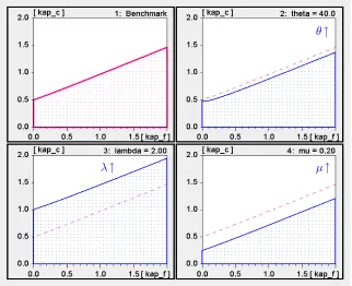
A summary of the stabilizing or destabilizing properties of the parameters can be made more vivid by computing the stability frontiers in a paremeter plane. Most expedient for this are the trading capitalsκf andκc of the two speculative groups, where now a greater

range of the two coefficients than in Figure 1 should be considered. To set up a benchmark of the other three parameters, we maintain the scaling λ = 1 for market liquidity and the market maker’s risk aversion µ = 0.05, and reduce the memory of chartists by half, i.e., we put θ = 20. The stability frontier in the (κf,κc) plane to which these coefficients give

rise is shown in the upper-left panel in Figure 2; it separates the pairs entailing stability (in the dotted area) from those entailing instability. Given that the functional expression

h in eq. (14) is fairly nonlinear in κc and κf, it is remarkable that the stability frontier is

an almost perfect straight line.

Proposition 3(d) has established that an originally stable equilibrium is destabilized by sufficiently long lagsθ, providedκc is contained in the intermediate interval (κf/2,(λ+κf)/2)

λ↑ µ↑ θ↑

Figure 2: Stability frontier of (PBT) in the (κf,κc) parameter plane.

Note: The dotted area is the stability region. The (red) dashed lines reproduce the stability frontier of the benchmark case in the first panel, which is based on λ = 1

µ= 0.05, θ= 20.

κc slightly less than 0.50 we have here the stability reswitching ofκf from Figure 1 (which

had θ = 40 underlying).

The other two panels in Figure 2 demonstrate the stabilizing effect when market liquidity is increased from 1 to λ= 2, and the destabilizing effect when the market maker’s risk aversion is increased from 0.05 to µ = 0.20. Again there are no ambiguities in the relocation of the stability frontier, practically it is even a parallel upward and downward shift, respectively. In sum, Figure 2 is a representative illustration of the fact that the parameter effects on stability are of an amazingly regular nature.

A special feature of the model is that we have an explicit expression for the cycle period

T induced by the parameters on the stability frontier,T = 2π/ν" _{according to Proposition}

of the model, we better resort to specific numerical values and make use of the stability frontiers already computed.

1: benchmark 2: θ = 40 (↑)

3: λ= 2.00 (↑)

4: µ= 0.20 (_↑)

Figure 3: Period T on the four stability frontiers from Figure 2.

Figure 3 depicts on the horizontal axis the same values of κf as in Figure 2. It takes

the parameters underlying the latter diagram, computes the bifurcation values of κc given

κf, plugs all these coefficients into the formula for ν", and then draws T = 2π/ν" as a

function of κf. Numbers 1. .4 in Figure 3 indicate the panels in Figure 2 from which the

functions are thus obtained. Since the second panel has examined a different lag θ from the other panels, Figure 3 plots the fraction T /θ.

One property that the four functions have in common is that they decline with κf.

Regarding the cycle prolonging effects of an increase in µit is interesting to quote a remark by Farmer on the market maker, although he made it in a stochastic context with no chartists: “Once the market maker acquires a position, because of her risk aversion, she has to get rid of it. By selling a fraction β [our coefficient µ] at each time step, she will unload the position a bit at a time. This behavior causes a trend in prices. Any risk-averse behavior on the part of the market maker will result in a temporal structure of some sort in prices.” (Farmer, 2001, p. 67). It is noteworthy that this tendency still prevails when we restrict our attention to the periodic orbits generated by the bifurcation values of the parameters.

One point following from these considerations is that temporal structure in prices creates an opportunity for technical traders (ibid., p. 68). This observation motivates us to have now a look at the time series properties of the model and, in particular, the implied performance of the agents.

3.4

Dynamic mechanisms over a cycle

While cycle generating feedbacks in models with order-based strategies are well understood, these aspects are still largely neglected in the position-based systems. For this reason we want to study a stylized cyclical motion of (PBT), without any random noise and unaffected by nonlinear amendments like thresholds and flexible ceilings and floors. It will also be illuminating to compare the cyclical patterns of the variables with those arising from the order-based Beja–Goldman model. The parameters that we employ to obtain periodic orbits of these linear systems read as follows:7

BG : φ = 0.20 χ = 2.000 βp = 1 βπ = 0.20

PBT : φ = 0.20 κc = 0.616 λ = 1 θ = 20 µ = 0.05

(16)

The results for the two models are contrasted in Figure 4, where the BG model is shown in the upper part and the PBT model in the lower part. Let us begin with system (BG), at a point in time when the price is rising and just passes the fundamental value, which is normalized at zero. This happens at t = 39.50 in the top panel of the diagram. Since the

7_{(PBT) is discretized with∆t= 1, which is not too large given the lagθ= 20. The bifurcation valueκ}

c

given the other parameters is slightly higher (not lower!) than it would be in continuous time. For (BG) the step size is so small that the continuous-time and discrete-time bifurcation values ofκc are practically

demand of fundamentalists is a negative mirror image of the price movements, the price increases are here solely due to the demand of the chartists. The latter is positive since the price has already been rising for a while, such that the perceived trend of the chartists has become positive in the meantime.

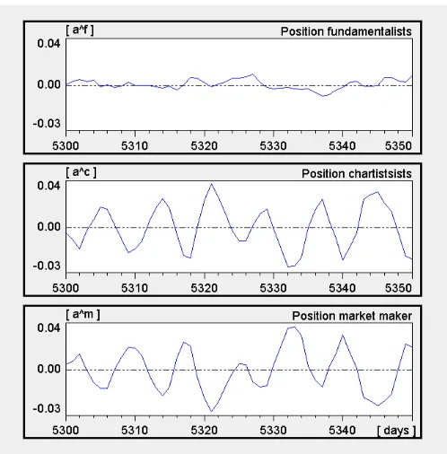
Figure 4: Price series and the agents’ characteristics in (BG) and (PBT).

Note: The bold (blue) line in the top panel of (BG) and (PBT), respectively, is the log price, the bold lines in the other panels depict market orders, or demands,df and dc_{. The thin solid (red) lines are the positions a}m_{, a}f_{, a}c_{, respectively, the dotted} (green) lines are the profit flows, or capital gains, gm, gf, gc. Market orders and

A central feature of the cycle generating mechanism in the BG model is the fact that the more the price increases, the stronger becomes the negative impact on the part of the fundamentalists. The ensuing slow down in the price increases works to the effect that eventually the rising trend as it is perceived by the chartists, π, comes to a halt and then begins to decline. Since this occurs at a relatively high level of π, chartist demand still exceeds fundamentalist demand for some time. At t = 47.38, the difference between the two narrows down to zero, so that ˙p = 0 and the price reaches an upper turning point. From then on p is falling; the decline in π accelerates and dc _{decreases faster as d}f _now

begins to increase. Hence the negative demand of the fundamentalists dominates the (here still positive) demand of the chartists. As the decline in the price goes on, the dynamics enters the stage with which we have begun, now with signs reversed.

Before discussing the implied positions and profits, let us turn to the lower part of Figure 4 with the dynamics of the PBT model. The initial conditions have been chosen such that with ±0.23 the price oscillations exhibit the same amplitude as in the BG model. We consider the same phase of a cycle as before, beginning with the upward movement of the price when it just crosses the zero line att = 1298. For the fundamentalists it is now the position af _{rather than the demand that is a negative mirror image of the price series; see}

the thin solid (red) line in the middle panel. Sinceaf _{is falling att = 1298, fundamentalist}

demand df _{= ˙a}f _{is initially negative. At that time it is even close to its trough value over}

the entire cycle. Note, however, that the amplitude ofdf _{in (PBT) is more than four times}

lower than in (BG), ±0.52 versus ±2.29.

In order for the price to increase att = 1298, chartist demand dc _{must dominate d}f_,

which can be seen in the bottom panel. The reason for the relatively high demand is not the positive position ac_{, which is proportional to the slope in the log price p(1298)−p(1278),}

but the fact that this slope is presently rising, so that ac _{is rising and thus d}c _{= ˙a}c _{> 0.}

In addition the negative inventory am _{of the market maker has to be taken into account,}

which viathe correction term ₋µam _{>0 in the price impact function (7) reinforces the rise}

inp.

In the next few periods there are two features that, taken on their own, would ac-celerate the price increase. First, the increase in the market maker’s short position, i.e., the ongoing decline in am_{. Second, the position of fundamentalists declines, too, but at a}

market tends to weaken. Chartist demand, however, counteracts these forces. Although chartists continue to build up long positions, they do this more and more slowly. In fact, their position reaches the highest level at t = 1310, afterwards ˙ac _{< 0 and chartists turn}

into net suppliers of the asset.

The price peaks three periods later, at t = 1313. Its increase over this short interval where both dc _{and d}f _{are negative is due to the market maker, who with his accumulated}

short position still feels it necessary to give some incentive to the agents to sell the asset to him.

The beginning downturn of the price gains momentum through the increasing desire of the chartists to cut down on their long position, though for a while they keep on wanting to hold the asset in positive amounts. Their supply is the main force on the market in that stage of the cycle, which dominates the low positive demand of the fundamentalists and the positive price correction by the market maker.

The discussion will have made it clear that with position-based strategies, even though it is a prototype model and we have only studied the most regular periodic trajectories, the dynamic relationships are more involved than in the Beja–Goldman model; since in addition to the relationship between demand and price changes, the relationships between the two speculative groups of agents, and the new influence of the market maker’s risk aversion, one also has to consider the relationships between the agents’ stock and flow variables, i.e., their desired positions and the market orders deriving from them.

It can moreover be said that fundamentalists and chartists perform different roles over the cycle in the two modelling frameworks. Thus, take the stage of the cycle when after the peak the price begins to fall. In the BG model this phase is characterized by the negative demand of the fundamentalists, which dominates the positive demand of the chartists. By contrast, in the present PBT model chartist and fundamentalist demands have opposite signs from BG, and it is the negative demand of the chartists which dominates the positive demand of fundamentalists and so causes the price to fall.

conditions. In the first three panels the initial values of am_{, a}f_{, a}c _{have therefore been}

chosen in such a way that the positions oscillate around zero; see the thin solid (red) lines in Figure 4, which have been suitably rescaled to let the cyclical patterns and comovements stand out more clearly.

With the time series of the price and the positions we can compute the profits from the different trading strategies. To ease the discussion, let us assume that the agents’ target positions are zero. Denoting the actual asset price by P = exp(p) and the value of the alternative asset that an agent h holds by mh_{, the wealth of this agent is given by}

Wh _{=P a}h_+mh_{. The changes inm}h _{are inversely related to the sales and purchases of the}

risky asset, i.e., ˙mh _{= −P d}h _=−Pa˙h_{. Hence the capital gains g}h _{of agent h from trading}

are determined by,8

gh = ˙Wh = ˙P ah+Pa˙h+ ˙mh = ˙P ah = exp(p) ˙pah h=f, c, m (17)

These profits are depicted as the dotted (green) lines in Figure 4. Regarding the BG model, it is obvious that the fundamentalists should make positive profits over a cycle; after all they consistently buy low and sell high. Even their instantaneous profits turn out to be positive whenever the price changes, since they have gone long when the price is rising and short when it is falling.

Chartists, by contrast, earn positive profits only over short subintervals of the cycle: in the upswing (downswing) of the price just after their position becomes positive (negative). As soon as the price reaches its peak or trough, respectively, the chartists make losses again. It may also be observed that although the oscillations of the price and the position appear almost perfectly symmetrical, the induced motions of the profits are not. The losses of chartists are heavier when their long position is deteriorated by the falling price than when their position is negative and the asset appreciates.

Averaging over a full cycle, the losses of the chartists turn out to be almost equal to the profits earned by the fundamentalists. Therefore, in the present stylized scenario, the market maker neither loses nor wins from his function as an intermediary. The reason for this is that profits in the aggregate cancel out, gf _+gc _+gm _{= 0 in every instant of time,}

which follows from (5).

The second part of Figure 4 demonstrates that relative profits in the PBT model are different from the BG model. The PBT dynamics allows both fundamentalists and chartists to make positive profits over the cycle, which goes at the expense of the market maker. The latter could, of course, make up for these losses by charging a fee on the transactions or by bid-ask spreads, which so far have not been explicitly modelled.

Besides the qualitative statements, the profits of fundamentalists and chartists cannot be unambiguously compared, since the coefficientsκf,κc, which for short have been referred

to as “trading capital”, incorporate the aggressiveness of single agents as well as the market fractions of the two groups. Hence if the almost ten times higher profits of the chartists that we obtain, gc_/gf _{= 930/95, were attributed to a ten times higher market fraction of}

this group, fundamentalist and chartist trading strategies would perform equally well. More informative in this respect is perhaps the ratio of the amplitudes of profits and positions, which are indeed almost equal:9 _gf_/af _{= 712/464 ≈ 1.5 versus g}c_/ac _{= 392/257 ≈ 1.5.}

Nevertheless, as long as both groups of speculative traders earn positive profits, unambigu-ous comparisons between the two can only be made across different parameter sets with identical coefficients κf and κc.

4

A stochastic version of the model

4.1

Properties of a base scenario

Financial market models with a more or less distant view to the empirical stylized facts are directly set up as stochastic models. Often, but not always, a deterministic skeleton is then identified and part of the investigation is concerned with the deterministic properties and how they may influence the statistical properties of the full model. The presentation in this paper is the other way around. After having designed a deterministic prototype model and studied its main features, we now proceed with a minimal stochastic extension. This means the model is formulated in discrete time (∆t= 1, so to speak) and we work with the widely employed assumption that the fundamental value follows a random walk.

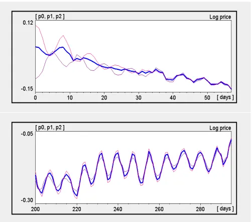
When establishing a numerical set of parameters that can serve as a base scenario and, in particular, in order to assess the memory θ of the chartists, the time unit of the model must be made explicit. To this end we make a visual inspection of several episodes of the S&P 500 stock price index that are not too much trending, so that they allow us to recognize some (noisy) cyclical patterns. We perceive an average length between 7 and 8 days of these cycles, whatever may have caused them or how spurious the phenomenon might be. On the other hand, the period of the oscillations of (PBT) in Figure 4 was 55 time units, and the period in the model that will be relevant to us shortly below is 53 time units. Therefore, we may stipulate that seven time units of the model correspond to one trading day.

In many simulations of financial markets with a random walk for the fundamental value, the latter is supposed to change every day. To be in line with this convention, the fundamental valuev=vtin PBT is updated, not every time unit, but everyτ= 7 time units.

Numerically we follow He and Li (2007, p. 3404), who adopt an annual volatility of 20%. The corresponding standard deviation for the daily changes of vt is σv = 0.20/

√

250 = 0.0126. The precise formulation of this discrete-time stochastic process is given in Appendix A.3 .

Of course, since nonlinearities continue to be absent in the model, only parameters entailing deterministic stability are admissible to simulate this market. Our idea is to maintain the basic cyclical tendencies we have found, so that the parameters should give rise to dampened oscillations in the deterministic version (as in He and Li, 2007, pp. 3404f). Specifically, starting out from the PBT parameters in (16) above, we decide to settle down on a set of rounded parameters that imply a dampening factor of 0.69 and a period of 53 time units, i.e. 7.57 days (defining the dampening factor as the ratio of two successive peak values of the log price). These parameters are collected in Table 2.

κf κc θ λ µ σv τ

0.20 0.57 20 1.00 0.050 0.0126 7

Table 2: Base scenario of the stochastic PBT model.

well comparable. For our investigations of the parameter effects below, this qualitative correspondence will be good enough.

Figure 5: Contrasting an artificial price series with S&P 500.

Note: Underlying the simulation run are the coefficients of Table 2. The bold (blue) line in the lower panel depicts the log price pt, the thin (green) line is the random walk of the fundamental value vt.

The lower panel in Figure 5 also illustrates that the price tracks the fundamental value rather closely (actually more closely than the examples given in Farmer, 2001, p. 67 and Farmer and Joshi, 2002, pp. 162f). Upon closer inspection of the price series over shorter time intervals, however, one could distinguish episodes where pt seeks to catch up with vt

very rapidly, and other episodes of 10 or 20 days where the temporarily divergent tendencies of the cycle generating mechanism prove to be dominant, so thatptandvtmove out of line.

The fact that the price does not deviate very far and not very persistently from the fundamental value implies that the positions af_t of the fundamentalists center around their target. Though it is analytically not obvious, it turns out that the basic convergence forces in the system are so strong that also the positions ac

t of the chartists are centered. This

notwithstanding, their amplitude can be quite variable over longer time intervals.

The short sample period of 50 days shown in Figure 6 can illustrate three things. First, the consistent centering of the agents’ positions. Second, the distinctly larger fluctuations ofac

t versusa f

Figure 6: Positions af_t,ac

t,amt over a short sample period in the base scenario.

is largely inversely related toac

t, which demonstrates that his main function is to buffer the

market disequilibria caused by the chartists. A third point is that the cyclical tendencies of the deterministic core manifest themselves, not so much in the price series with its pseudo trend incidents, but at the level of the positions of the chartists and the market maker.

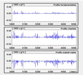
Regarding the capital gains that the agents derive from their positions, the regular oscillations in Section 3.4 proved to yield positive profits over the cycle for fundamentalists as well as for chartists, which goes at the expense of the market maker. Figure 7 makes it evident that, in the long-run, this also holds true in the stochastic setting, at least at the present parameter values. Precisely, the diagram presents the daily profits of agent group

h, gh

t =Wth−Wth−τ with τ= 7 (period t a multiple ofτ) and h=f, c, m.

The high spikes in the middle panel for the chartists might suggest that the profits from ac

t are much higher than the profits from a f

t, similar perhaps to the ratio 930/95

Figure 7: Daily profits g_tf, gc

t, gtm of the agents in the base scenario.

could be argued that fundamentalism and chartism are about equally attractive, since the higher profits gc

t come along with a higher standard deviation, 6.29 versus 2.71 forg f t (and

7.51 versus 2.88 in Figure 7). Note that in both cases the positive mean values are not much more than one third of the standard deviation. So chartist and also fundamentalist trading is not without risk—at least if the initial wealth is small or trading is debt financed. It will also be observed that for the chartists tranquil times alternate with larger fluctuations of the profits. This phenomenon may be informally described as volatility clustering. Nevertheless, it must then not be forgotten that we are concerned with profits, and here the profits of only one of the speculative groups. Volatility clustering of returns, to which this mode of expression usually applies, is not yet achieved; in this respect the model is still too simple.

4.2

A stochastic equilibrium notion

the transition probabilities P(dt, B) that a price deviation dt:=pt−vt in period t will, in

the next period t+1, be contained in the set B. The period-t variable to be studied will then be a time-varying unconditional probability distribution πt of dt. If its law of motion

is succinctly summarized by a mapping Φ, such that πt+1 = Φ(πt), an equilibrium of this

process is constituted by an invariant distribution π" _{satisfying the equation π}" _{= Φ(π}"_).

Under certain regularity conditions, which one feels should be satisfied here, such a fixed point exists, is unique, and is attractive, i.e., πt →π" ast→ ∞ for any initial distribution

π0.10

If this kind of ergodicity prevails, the qualitative long-run behaviour of each sample path of the system is completely described by the Markov equilibrium from a statistical point of view. It does not, however, describe the quantitative behaviour of single sample paths nor the qualitative behaviour of ensembles of sample paths, whether sample paths starting at different states converge or diverge for a given sequence of random shocks. An appropriate concept to treat this problem is that of a random fixed point and its asymp-totic stability, which are counterparts of the deterministic concepts. It is, in particular, convenient that this notion of stability is one of pointwise convergence.

In its precise definition, a random fixed point is a random variable, that is, a mapping on a probability space, which is a rather abstract and technical concept.11 _{For the present}

purpose it is sufficient to degenerate the probability space to a given sequence{δt}∞t=0 of the

random walk innovations to the fundamental value. In this perspective, the stochastic model becomes a forced oscillator, which has a deterministic solution path once an initial price history is given. An implication of a random fixed point, then, is that the solutions from any two price histories get, and stay, arbitrarily close as time unfolds. As a consequence, all these sample paths have the same limiting behaviour.12

10_{Such a result should at least be obtainable if the normal distribution for the innovations in the random} walk is truncated. For a compact introduction to the these discrete-time Markov processes with continuous state space, and the conditions for uniqueness of and convergence towardπ!_{, see Futia (1982),}

11_{Arnold (1998) is a standard reference to the theory of random dynamical systems. For an immediate} in-troduction to random fixed points and applications to economic systems, see Schenk–Hopp´e and Schmalfuß (2001), and B¨ohm and Chiarella (2005).

Figure 8: Convergence of sample paths from different initial conditions.

Note: The upper panel has the base scenario underlying with, in particular,κc = 0.57. In the lower panel this parameter is changed to κc = 0.61, which is close to the bifurcation value.

Figure 8 illustrates the convergence process to the limiting behaviour for the base scenario of Table 2. Actually, convergence is rather fast, after 40 days the three price series are virtually identical. A lower speed of convergence will, however, be expected if the parameters are closer to the stability frontier. This intuition is confirmed in the lower part of Figure 8, where with κc = 0.61 the chartist trading capital is only marginally below its