WORKING PAPERS SERIES
WP04-17
Estimating and Testing Stochastic
Estimating and Testing Stochastic Volatility Models using Realized
Measures
∗Valentina Corradi†
Queen Mary, University of London
Walter Distaso‡ University of Exeter
October 2004
Abstract
This paper proposes a procedure to test for the correct specification of the functional form of the volatility process, within the class of eigenfunction stochastic volatility models (Meddahi, 2001). The procedure is based on the comparison of the moments of realized volatility measures with the corresponding ones of integrated volatility implied by the model under the null hypothesis. We first provide primitive conditions on the measurement error associated with the realized measure, which allow to construct asymptotically valid specification tests.
Then we establish regularity conditions under which realized volatility, bipower variation (Barndorff -Nielsen & Shephard, 2004d), and modified subsampled realized volatility (Zhang, Mykland & A¨ıt Sahalia, 2003), satisfy the given primitive assumptions.
Finally, we provide an empirical illustration based on three stock from the Dow Jones Industrial Average.
Keywords: generalized method of moments, eigenfunction stochastic volatility model, integrated volatility, jumps, realized volatility, bipower variation,
microstructure noise. JEL classification: C22, C12, G12.
∗We wish to thank the editor, Bernard Salani´e, two anonymous referees, and Karim Abadir, Andrew Chesher, Atsushi Inoue, Paul Labys, Oliver Linton, Enrique Sentana, Ron Smith, as well as the seminar participants at the 2003 Winter meeting of Econometric Society in Washington DC, the 2003 Forecasting Financial Markets Conference in Paris, the 2003 Money, Macro and Finance Conference at London Metropolitan University, LSE-Financial Market Group, the 2003 CIREQ-CIRANO Realized Volatility Conference at University of Montreal, IFS-UCL, Rutgers University and Universit`a di Bari for very helpful comments. We are particularly indebted to Nour Meddahi and Peter Phillips for helpful suggestions on a previous version of the paper. The authors gratefully acknowledge financial support from the ESRC, grant code R000230006.
†Queen Mary, University of London, Department of Economics, Mile End, London, E14NS, UK, email:
‡University of Exeter, Department of Economics, Streatham Court, Exeter EX4 4PU, UK, email:
1
Introduction
Modelling, estimation and testing of financial volatility models has received increasing attention over the recent years, from both a theoretical and an empirical perspective. In fact, accurate specification of volatility is of crucial importance in several areas of financial risk management, such as Value at Risk, and in hedging and pricing of derivatives. Asset prices are typically modelled as diffusion processes; such processes are fully characterized by the drift and volatility function, which describe the conditional instantaneous mean and variance of the asset price. The volatility term has often been modelled as a function of some latent factors, which are also described by diffusion processes.
The specification of the functional form of such diffusion processes has been suggested by eco-nomic theory, often constrained by the need of mathematical tractability. Hence the need of devising statistical procedures to test whether a chosen model is consistent with the data at hand.
Several tests have been proposed for the correct specification of the full model, thus including both the drift term and the variance term. A frequently used approach consists in simulating the model under the null hypothesis using a fine grid of parameters values, and then sampling the simulated data at the same frequency of the actual data; one can then obtain an estimator by either minimizing the distance between sample moments of actual and simulated data, as in simulated generalized method of moments (see Duffie & Singleton, 1993), or minimizing the expectation, under the simulated model, of the score of some auxiliary model, as in the efficient method of moments (see e.g. Gallant & Tauchen, 1996; Gallant, Hsieh & Tauchen, 1997; Chernov, Gallant, Ghysels & Tauchen, 2003). Both simulated generalized and efficient method of moments lead to tests for the validity of overidentifying restrictions, whose rejection gives some information about the deficiencies of the tested model. Recently, Altissimo & Mele (2003) have suggested a new estimator based on the minimization of the weighted distance between a kernel estimator of the actual data and of the simulated data. Then, a test based on the difference of the two estimated densities can be constructed.
Another approach consists in testing the distributional assumptions implied by the model under the null hypothesis. For example, Corradi & Swanson (2003) suggest a test based on the comparison of the empirical cumulative distribution function of the actual and of the simulated data; Hong & Li (2003) and Thompson (2002) propose tests based on the probability integral transform, exploiting the fact that if F(Xt|Ft) is the true conditional distribution of Xt, then F(Xt|Ft) is distributed
as an i.i.d.uniform random variable on [0,1]; and Bontemps & Meddahi (2003a,b) propose testing
An alternative approach is to test only for the volatility process, given that, in several instances, such as hedging and pricing of derivative assets, particular interest lies in the specification of the variance term.1 However, in this case one cannot directly compare actual and simulated volatility
moments, or the empirical distribution of actual and simulated volatility, given that the volatility process is not observable. Over the past, squared returns have been a frequently used proxy for volatility. Unfortunately, as pointed out by Andersen & Bollerslev (1998), squared returns are a very noisy proxy for volatility. Implied volatilities, obtained by inverting the option price formulae, are another popular proxy, but are model dependent and incorporate some price of risk, indicating the expected future volatility.
Hence, the need for accurate and model free measures of volatility. Over the last few years there has been great progress in this direction. A new proxy for volatility, termed realized volatility, has been introduced concurrently by Andersen, Bollerslev, Diebold & Labys (2001, 2003) and by Barndorff-Nielsen & Shephard (2001, 2002, 2004a,b), who have provided the relevant limit theory and extensions to the multidimensional case. Assuming that we have M recorded intraday
observations for a given asset price process, over a given day, realized volatility is computed by summing up the M squared returns. If prices have continuous paths and are not contaminated by
microstructure noise, then realized volatility is a consistent estimator of daily integrated volatility. It is often believed, though, that (log) price processes may display jumps, due for example to macroeconomic and financial announcement effects. Barndorff-Nielsen & Shephard (2004d) have recently introduced a new realized measure, called bipower variation, which is consistent for integrated volatility when the underlying price process exhibits occasional large jumps.
Finally, Zhang, Mykland & A¨ıt Sahalia (2003) have suggested a new realized measure, hereafter termed modified subsampled realized volatility, which is consistent for integrated volatility when prices are contaminated by microstructure noise.
The availability of these model free measures of integrated volatility immediately suggests their use for testing some parametric models, by comparing some features of the realized measures with those of the model.
This is the object of this paper. Within the class of eigenfunction stochastic volatility models (Meddahi, 2001), which nests all the most popular stochastic volatility models as special cases, this paper proposes a procedure to test for the correct specification of the functional form of the volatility process. The procedure is based on the comparison of the moments of the realized measures with
1Recall that over a finite time span, the contribution of the drift term is indeed negligible. Specification test for
the corresponding ones of integrated volatility implied by the tested model.
The idea of using moment conditions for estimating and testing stochastic volatility models using realized measures is not new. In fact, Bollerslev & Zhou (2002) have derived analytically the first two conditional moments of the latent volatility process, for the class of affine stochastic volatility models. Then they suggested a generalized method of moments estimator and an associated test for the validity of overidentifying restrictions based on the comparison between the analytical conditional moments of integrated volatility and the corresponding sample moments of realized volatility. Bollerslev & Zhou consider the case of the time spanT approaching infinity, for a given
number of intraday observationsM.The effects of various values ofM on the properties of the test
are analyzed via a Monte Carlo simulation.
The present paper extends Bollerslev & Zhou’s in three directions. First, we consider a double asymptotic theory in which bothT andM approach infinity, and we provide regularity conditions
on their relative rate of growth. Second, we also consider tests comparing (simulated) moments of integrated volatility with sample moments of bipower variation, thus allowing for possible jumps, and with sample moments of modified subsampled realized volatility, thus allowing for at least some classes of microstructure noise. Finally, we do not confine our attention to affine stochastic volatility models, but we consider the class of eigenfunction stochastic volatility models of Meddahi (2001), where the latent volatility process is modelled as a linear combinations of the eigenfunctions associated with the infinitesimal generator of the diffusion driving the volatility process.
The main reason why we focus on Meddahi’s eigenfunction stochastic volatility class is that it ensures that the integrated volatility process has a memory decaying at a geometric rate and has an ARMA(p, p) structure, when the number of eigenfunctions,p, is finite (see Andersen, Bollerslev
& Meddahi, 2002, 2004; Barndorff-Nielsen & Shephard, 2001, 2002); and that the measurement error associated with the realized measures has a memory decaying at a fast enough rate. These features are crucial, as in our context bothT andM approach infinity.
Indeed, it should be stressed that Barndorff-Nielsen & Shephard (2004a) provide a central limit theorem for the measurement error associated with realized volatility, which holds for a very general class of semimartingale processes. However, their result concerns the fixed time span case, and thus there is no need to impose restrictions on the degree of memory of the volatility process. Of course, if one wishes to construct a testing procedure based on a finite time span, there is no need to consider a specific class of models, and then he can benefit from the generality of Barndorff-Nielsen & Shephard’s result.
the time span can approach infinity, in relation to the rate at which the moments of measurement error approach zero. Section 4 considers the case in which there is no explicit closed form for the moments of integrated volatility. For this case we propose a simulated version of the test based on the comparison of the sample moments of realized measures and sample moments of the simulated integrated volatility process. We also discuss the possibility of constructing a test based on the comparison of sample moments of actual and simulated realized measure, for fixedM. Section 5
provides conditions under which realized volatility, bipower variation and modified subsampled realized volatility satisfy the primitive conditions on the measurement error. In particular, it is emphasized that the rate at which T can grow, relatively to M, differs across the three realized
measures. Section 6 provides an empirical illustration of the suggested procedure, based on data on different stocks of the Dow Jones Industrial Average. Finally, Section 7 concludes. All the proofs are gathered in the Appendix.
2
The Model
The observable state variable, Yt = logSt, where St denotes the price of a financial asset or the
exchange rate between two currencies, is modelled as a jump diffusion process with a constant drift term. According to the eigenfunction stochastic volatility class, the variance term is modelled as a measurable function of a latent factor,ft,which is also generated by a diffusion process. Thus,
dYt=mdt+ dzt+
!
σ2
t
"#
1−ρ2dW
1,t+ρdW2,t
$
(1)
and
σt2=ψ(ft) = p
%
i=0
aiPi(ft) (2)
dft=µ(ft,θ)dt+σ(ft,θ)dW2,t, (3)
for some θ ∈ Θ ∈ R2p+1, where W
1,t and W2,t refer to two independent Brownian motions, the
parameter ρ ∈ [0,1) allows for leverage effects and Pi(ft) denotes the i-th eigenfunction of the
infinitesimal generator A associated with the unobservable state variable ft.2 The pure jump
process dzt specified in (1) is such that
Yt=mt+
& t
0 #
σ2
s
"#
1−ρ2dW
1,s+ρdW2,s
$
+
Nt
%
i=1
ci,
2The infinitesimal generator
Aassociated withft is defined by
Aφ(ft)≡µ(ft)φ"(ft) +
σ2(f
t)
2 φ ""(f
t)
for any square integrable and twice differentiable functionφ(·). The corresponding eigenfunctions Pi(ft) and
eigen-values−λiare given byAPi(ft) =−λiPi(ft). For a detailed discussion and analysis on infinitesimal generators and
whereNtis a finite activity counting process, andciis a nonzero i.i.d.random variable, independent
ofNt. As Ntis a finite activity counting process, we confine our attention to models characterized
by a finite number of jumps over any fixed time span.
As customary in the literature on stochastic volatility models, the volatility process ia assumed to be driven by (a function of) the unobservable state variableft. Rather than assuming an ad hoc
function forψ(·), the eigenfunction stochastic volatility model adopts a more flexible approach. In
factψ(·) is modelled as a linear combination of the eigenfunctions ofAassociated withft. Notice
that the ai’s are real numbers and thatp may be infinite. Also, for normalization purposes, it is
further assumed that P0(ft) = 1 and that var (Pi(ft)) = 1, for any i $= 0. When p is infinite,
we also require that '∞
i=0a2i < ∞. The generality and embedding nature of the approach just
outlined stems from the fact that any square integrable function ψ(ft) can be written as a linear
combination of the eigenfunctions associated with the state variable ft. As a result, most of the
widely used stochastic volatility models can be derived as special cases of the general eigenfunction stochastic volatility model. For more details on the properties of these models, see Meddahi (2001) and Andersen, Bollerslev & Meddahi (2002) (hereafter ABM2002).
Finally, notice that we have assumed a constant drift term. This is in line with Bollerslev & Zhou (2002), who assume a zero drift term and justify this with the fact that there is very little predictive variation in the mean of high frequency returns, as supported the empirical findings of Andersen & Bollerslev (1997). Indeed, the test statistics suggested below do not require the knowledge of the drift term. However, some of the proofs make use of the fact that the drift is constant.
Following the widespread consensus that transaction data occurring in financial markets are of-ten contaminated by measurement errors, we assume to have a total ofM T observations, consisting
of M intradaily observations forT days, for
Xt+j/M =Yt+j/M +$t+j/M, t= 1, . . . , T and j= 1, . . . , M,
where
$t+j/M ∼i.i.d.(0,ν) and E($t+j/MYs+i/M) = 0 for all t, s, j, i. (4)
Thus, we allow for the possibility that the observed transaction price can be decomposed into the efficient one plus a “noise” due to measurement error, which captures generic microstructure effects. The microstructure noise is assumed to be identically and independently distributed and inde-pendent of the underlying prices. This is consistent with the model considered by A¨ıt Sahalia, Myk-land & Zhang (2003), Zhang, MykMyk-land & A¨ıt Sahalia (2003), Bandi & Russell (2003a,b).3 Needless
to say, whenν = 0,then$t+j/M = 0 (almost surely), and thereforeXt+j/M =Yt+j/M (almost surely).
3Recently, Hansen & Lunde (2004) address the issue of time dependence in the microstructure noise, while
The daily integrated volatility process at dayt is defined as
IVt=
& t t−1
σs2ds, (5)
where σ2
s denotes the instantaneous volatility at time s. Proposition 4.1 in ABM2002 gives the
complete moment structure of integrated volatility
E(IVt(θ)) =a0
var(IVt(θ)) = 2'pi=1
a2
i
λ2
i (exp(−
λi) +λi−1)
cov(IVt(θ), IVt−k(θ)) ='pi=1a2i exp (−λi(k−1))(1−exp(−λi))
2
λ2
i ,
(6)
This set of moments provides the basis for the testing procedure derived in the next Sections. In particular, since IVt is not observable, different realized measures, based on the sample Xt+j/M,
t = 1, . . . , T and j = 1, . . . , M, are used as proxies for it. The realized measure, sayRMt,M, is a
noisy measure of the true integrated volatility process; in fact
RMt,M =IVt+Nt,M,
where Nt,M denotes the measurement error associated with the realized measure RMt,M. Note
that, in the case whereν >0, any realized measure of integrated volatility is contaminated by two
sources of measurement errors, given that it is constructed using contaminated data.
Our objective is to compare the moment structure of the chosen realized measureRMt,M with
that ofIVt given in (6). Note that whenp= 1,cov(IVt(θ), IVt−k1(θ))/cov(IVt(θ), IVt−k2(θ)) =
exp(−λ1(k1−k2)),so that, by using mean, variance and two autocovariances ofIVt(θ), we obtain
one overidentifying restriction. Analogously, when p = 2, we shall be using four autocovariances,
as well as mean and variance, in such a way to obtain one overidentifying restriction.4 In order
to test the correct specification of a given eigenfunction volatility model, we impose the particular parametrization implied by the model under the null hypothesis.
In the sequel, we will first provide primitive conditions on the measurement errorNt,M, in terms
of its moments and memory structure, for the asymptotic validity of tests based on the comparison of the moments of RMt,M with those of IVt. Then, we shall adapt the given primitive conditions
on Nt,M to the three considered realized measures of integrated volatility: namely,
(a) realized volatility, defined as
RVt,M = M%−1
j=1 (
Xt+(j+1)/M−Xt+j/M)2; (7)
4However, note that whenp= 2,in the case of Ornstein-Uhlenbeck and affine processes,λ
2 = 2λ1.Thus, in this
(b) normalized bipower variation, defined as
(µ1)−2BVt,M = (µ1)−2
M M −1
M%−1
j=2 *
*Xt+(j+1)/M −Xt+j/M****Xt+j/M−Xt+(j−1)/M** (8)
whereµ1 = E|Z|= 21/2Γ(1)/Γ(1/2) and Z is a standard normal distribution;
(c) modified subsampled realized volatility, defined as
+
RVut,l,M =RVt,l,Mavg −2lν,t,M, (9)
where
,
νt,M =
RVt,M
2M =
1 2M
M%−1
j=1 (
Xt+(j+1)/M−Xt+j/M
)2
,
RVt,l,Mavg = 1 B
B
%
b=0
RVt,l,Mb = 1 B
B%−1
b=0
M−(%B−b−1)
j=b+1 (
Xt+jB/M−Xt+(j−1)B/M)2, (10)
and Bl∼=M;ldenotes the subsample size and B the number of subsamples.
In particular, for each considered realized measure we will provide regularity conditions for the rel-ative speed at whichT, M, l go to infinity for the asymptotic validity of the associated specification
test for integrated volatility.
In the remainder of the paper, two main cases will be considered. The first is when explicit formulae for the moments of the integrated volatility are available, and so the map between the parameters (a0, . . . , ap,λ1, . . . ,λp) and the parameters describing the volatility diffusion in (2) is
known in closed form; the second case is when explicit formulae for the moments of the integrated volatility are not available. As detailed in the following section, in the first case the parameters of the model will be estimated with a generalized method of moments estimator, while in the second case a simulated method of moments estimator will be employed.
3
The case where the moments are known explicitly
When explicit formulae for the moments of the integrated volatility are available, and so is the map between the parameters (a0, . . . , ap,λ1, . . . ,λp) and the parameters describing the volatility
diffusion in (2), we can immediately write the set of moment conditions as
gT,M(θ) =
1
T
T
%
t=1
= 1 T 'T
t=1RMt,M −E(IV1(θ)) 1
T
'T t=1
(
RMt,M −RMT,M
)2
−var(IV1(θ)) 1
T
'T t=1
(
RMt,M −RMT,M) (RMt−1,M−RMT,M)−cov(IV1(θ), IV2(θ))
... 1 T 'T t=1 (
RMt,M −RMT,M) (RMt−k,M−RMT,M)−cov(IV1(θ), IVk+1(θ)) ,
where RMT,M =T−1'Tt=1RMt,M and the moments of integrated volatility are computed under
the volatility model implied by the null hypothesis. The generalized method of moments (GMM) estimator can be defined as the minimizer of the quadratic form
,
θT,M = arg min
θ∈ΘgT,M(θ)
$W−1
T,MgT,M(θ). (12)
The weighting matrix in (12) is given by
WT,M =1
T T % t=1 ( g∗
t,M −g∗T,M
) (
g∗
t,M −g∗T,M
)$ (13)
+ 2 T pT % v=1 wv T %
t=v+1 (
g∗
t,M −g∗T,M
) (
g∗
t−v,M −g∗T,M
)$
,
wherewv = 1−pTv−1,pT denotes the lag truncation parameter, g∗T,M =T−1
'T
t=1g∗t,M and
g∗ t,M = RMt,M (
RMt,M −RMT,M)2
(
RMt,M −RMT,M
) (
RMt−1,M −RMT,M
)
...
(
RMt,M −RMT,M
) (
RMt−k,M −RMT,M
) . (14)
Note that the vector gT,M(θ) is (2p+ 2)×1, while the parameter space Θ ∈R2p+1; therefore the
use of gT,M(θ) in estimatingθ imposes one overidentifying restriction.
Indeed, GMM is not the only available estimation procedure. For example, Barndorff-Nielsen & Shephard (2002) suggested a Quasi Maximum Likelihood Estimator (QMLE) using a state-space approach, based on the series of realized volatilities. Thus, QMLE explicitly takes into account the measurement error between realized and integrated volatility. In the present context, we limit our attention to (simulated) GMM, as our objective is to provide a specification test based on the validity of overidentifying restrictions.
We can define the minimizer of the limiting quadratic form
θ∗ = arg min θ∈Θg∞(θ)
$W−1
∞g∞(θ), (15) whereg∞(θ) andW−∞1are the probability limits, asT andM go to infinity, ofgT,M(θ) andWT,M−1 ,
Hereafter, we shall test the following hypothesis
H0 :g∞(θ∗) =0 versus HA:g∞(θ∗)$=0. (16)
Note that correct specification of the integrated volatility process implies the satisfaction of the null hypothesis. On the other hand, the test does not have power against a possible stochastic volatility eigenfunction model leading to an integrated volatility having the same first two moments and the same covariance structure as that implied by the null model.
In the sequel, we shall need the following set of assumptions.
Assumption A1: There is a sequencebM,withbM → ∞ asM → ∞,such that, uniformly in t,
(i) E (Nt,M) =O(b−M1),
(ii) E"Nt,M2 $=O(b−M1),
(iii) E"N4
t,M
$
=O(b−M3/2),
(iv) either
(a) Nt,M is strong mixing with size−r, where r >2; or
(b) E (Nt,MNs,M) =O(bM−2) +αt−sO(bM−1),where αt−s=O(|t−s|−2).
Assumption A2: ft is a time reversible process.
Assumption A3: the spectrum of the infinitesimal generator operator A of ft is discrete, and
denoted by λ0 = 0<λ1 < . . . <λi <λi+1, wherei∈N and −λi is the eigenvalue associated with
thei−th eigenfunction Pi(ft).
Assumption A4: Θ is a compact set of R2p+1,with pfinite
Assumption A5:
(i) θ,T,M and θ∗ are in the interior ofΘ,
(ii) E (∂gt,M(θ)/∂θ|θ∗) is of full rank,
(iii) g∞(θ)$W∞−1g∞(θ) has a unique minimizer.
Assumption A1 states some primitive conditions on the measurement error Nt,M. Basically, it
requires that its first, second and fourth moments approach zero at a fast enough rate asM → ∞,
and that E(Nt,MNt−k,M) declines to zero fast enough as both |k|, M → ∞. As we shall see in
Section (), the rate at whichb−M1 declines to zero depends on the specific realized measure we use.
Assumptions A2 and A3 are the assumptions used by Meddahi (2001, 2002b) and by ABM2002 for the moments and covariance structure of IVt(θ). One-dimensional diffusions are stationary and
that the infinitesimal generator operator is compact (Hansen, Scheinkman & Touzi, 1998) and is satisfied, for example, in the square root or the log-normal volatility models.5
The test statistic for the validity of moment restrictions is given by
ST,M =TgT,M(θ,T,M)$WT,M−1 gT,M(θ,T,M). (17)
The following Theorem establishes the limiting distribution ofST,M under the null hypothesis and
consistency of the associated test.
Theorem 1. Let A1-A5 hold. If as T, M → ∞, T /b2
M → 0, pT → ∞ and pT/T1/4 → 0, then,
under H0,
ST,M −→d χ21,
and, underHA,
Pr(T−1|ST,M|>ε
)
→1, for some ε>0.
Notice that we require that T grows at a slower rate than b2
M. Thus, the slower is the rate of
growth ofbM,the stronger is this requirement. The rate of growth of bM depends on the specific
realized measure RMt,M used and will be specified explicitly in Section 5.
As usual, once the null is rejected, inspection of the moment condition vector provides some insights on the nature of the violation.
Remark 1. Recently, Barndorff-Nielsen & Shephard (2004a) have provided a feasible central limit theorem for realized volatility and realized covariance valid for general continuous semimartingale processes, allowing for generic leverage effects. More precisely, they show thatM1/2(RV
T M −IVT
)
has a mixed normal limiting distribution, whenM → ∞andT is fixed. Thus, Barndorff-Nielsen &
Shephard’s feasible central limit theorem applies to the case in which the discrete interval between successive observations approaches zero and the time span remains fixed. In this paper we deal with a double asymptotics in which bothT andM go to infinity, and in order to have a valid limit
theory we first need to show that
1
√ T
T
%
t=1
(RMt,M −E(RMt,M)) =
1
√ T
T
%
t=1
(IVt−E(IVt)) +op(1)
and then that T−1/2'Tt=1(IVt−E(IVt))) satisfies a central limit theorem. For this reason, we
need that the memory of IVt and of Nt,M declines at a sufficiently fast rate. This is ensured by
the class of stochastic eigenfunction volatility models; in fact, in this class integrated volatility has a memory decaying at a geometric rate and has an ARMA(p, p) structure, when the number of
eigenfunctions,p, is finite.
5The spectral decomposition of multivariate diffusion is analyzed by Hansen & Scheinkman (1995) and by Chen,
4
The case where the moments are not known explicitly
The testing procedure suggested above requires the knowledge of the specific functional form of the eigenvalues and of the coefficients of the eigenfunctions,λi and a0, ai, i= 1, . . . , p, in terms of the
parameters characterizing the volatility process under the null hypothesis.
For the case where this information is not available, we can nevertheless construct a test based on the comparison between the sample moments of the observed volatility measure and the sample moments of simulated integrated volatility. If the null hypothesis is true, the two sets of moments approach the same limit, asT andM approach infinity, otherwise they will converge to two different
sets of limiting moments.
As one can notice from (12), a test for the correct specification of mean, variance and covariance structure of integrated volatility can be performed without knowledge of the leverage parameterρ and/or the (return) drift parameter m. This is because we rule out the possibility of a feedback
effect from the observable state variable to the unobservable volatility. Then, our objective is to approximate by simulation the first two moments and a given number of covariances (depending on the number of eigenfunctions of the model under the null hypothesis) of the daily volatility process. This is somewhat different from the situation in which we simulate the path of the process describing (the log of) the price of the financial asset, we sample the simulated paths at the same frequency as the data, and then we match (functions of) the sample moments of the data and of the simulated data using only observations at discrete time t = 1, . . . , T. In fact, in the latter
case it suffices to ensure that, for t = 1, . . . , T, the difference between the simulated skeleton
and the simulated continuous trajectories is approaching zero, in a mean square sense, as the sampling interval approaches zero. Broadly speaking, in the latter case it suffices to have a good approximation of the continuous trajectory only at the same frequency of the data, i.e. at t =
1, . . . , T.
On the other hand, in the current context, this does no longer suffice as we need to approximate all the path, given that daily volatility (say from t−1 to t) is defined as the integral of
(instan-taneous) volatility over the intervalt−1 and t. Pardoux and Talay (1985) provide conditions for
uniform, almost sure convergence of the discrete simulated path to the continuous path, for given initial conditions. However, such a result holds only on a finite time span. The intuitive reason is that the uniform, almost sure convergence follows from the modulus of continuity of a diffusion (and of the Brownian motion), which holds only over a finite time span.
Therefore we shall proceed in the following manner. For any valueθin the parameter spaceΘwe
simulate a path of lengthk+1,wherekis the highest order autocovariance that we want to include
hypothesis. Such invariant distribution is indeed known in most cases; for example it is a gamma for the square root volatility and it is an inverse gamma for the GARCH-diffusion volatility. Also, at least in the univariate case, we always know the functional form of the invariant density. For each θ ∈Θ, we simulate S paths of length k+ 1,for S sufficiently large. We then construct the
simulated sample moments by averaging overS the relevant quantities. More formally we proceed
as follows.
For any simulation i= 1, . . . , S, forj= 1, . . . , N and for anyθ∈Θ,we simulate the volatility
paths of lengthk+ 1 using a Milstein scheme, i.e.
fi,jξ(θ) = fi,(j−1)ξ(θ) +µ(fi,(j−1)ξ(θ),θ)ξ− 1
2σ$(fi,(j−1)ξ(θ),θ)σ(fi,(j−1)ξ(θ),θ)ξ +σ(fi,(j−1)ξ(θ),θ)(Wjξ−W(j−1)ξ
)
(18)
+1
2σ$(fi,(j−1)ξ(θ),θ)σ(fi,(j−1)ξ(θ),θ)
(
Wjξ−W(j−1)ξ
)2
,
where σ$(·) denotes the derivative of σ(·) with respect to its first argument, 3Wjξ−W(j−1)ξ
4
is i.i.d.N(0,ξ),fi,0(θ) is drawn from the invariant distribution of the volatility process under the null
hypothesis, and finallyNξ =k+ 1. For each i it is possible to compute the simulated integrated
volatility as
IVi,τ,N(θ) =
1
N/(k+ 1)
N/%(k+1)
j=1
σ2i,τ−1+jξ(θ), τ = 1, . . . , k+ 1, (19)
whereN/(k+ 1) =ξ−1,assumed to be an integer for the sake of simplicity, and
σi,2τ−1+jξ(θ) =ψ(fi,τ−1+jξ(θ)).
Also, averaging the quantity calculated in (19) over the number of simulations S and over the
length of the pathk+ 1 yields respectively
IVS,τ,N(θ) =
1
S
S
%
i=1
IVi,τ,N(θ),
and
IVS,N(θ) =
1
k+ 1
k+1 %
τ=1
IVS,τ,N(θ).
We are now in a position to define the set of moment conditions as
g∗
T,M −gS,N(θ) =
1
T
T
%
t=1
g∗
t,M −
1
S
S
%
i=1
whereg∗
t,M is defined as in (14) and
1
S
S
%
i=1
gi,N(θ) =
1
S
'S
i=1IVi,1,N(θ) 1
S
'S i=1
(
IVi,1,N(θ)−IVS,N(θ)
)2
1
S
'S i=1
(
IVi,1,N(θ)−IVS,N (θ)) (IVi,2,N(θ)−IVS,N(θ))
...
1
S
'S i=1
(
IVi,1,N(θ)−IVS,N(θ)) (IVi,k+1,N(θ)−IVS,N(θ))
. (21)
Similarly to the case analyzed in the previous Section, it is possible to define the simulated method of moments estimator as the minimizer of the quadratic form
,
θT,S,M,N = arg min
θ∈Θ(g
∗
T,M −gS,N(θ))$WT,M−1 (g∗T,M−gS,N(θ)), (22)
whereW−1
T,M is defined in (13). Also, define
θ∗ = arg min θ∈Θ(g
∗
∞−g∞(θ))$W∞−1(g∗∞−g∞(θ)), (23)
where g∗
∞,g∞(θ) andW−∞1 are the probability limits, asT,S, M and N go to infinity, of g∗T,M,
gS,N(θ) andW−T,M1 , respectively.
Finally, the statistic for the validity of the moment restrictions is given by
ZT,S,M,N =T
"
g∗
T,M −gS,N
" ,
θT,S,M,N
$$$
W−1
T,M
"
g∗
T,M −gS,N
" ,
θT,S,M,N
$$
. (24)
Analogously to the case in which the moment conditions were known, we consider the following hypothesis
H0: (g∗∞−g∞(θ∗)) =0 versus HA: (g∗∞−g∞(θ∗))$=0.
Before moving on the study of the asymptotic properties of ZT,S,M,N we need some further
assumptions.
Assumption A6: The drift and variance functions µ(·) and σ(·), as defined in (3), satisfy the
following conditions:
(1a) |µ(fr(θ1),θ1)−µ(fr(θ2),θ2)|≤K1,r+θ1−θ2+,
|σ(fr(θ1),θ1)−σ(fr(θ2),θ2)|≤K2,r+θ1−θ2+,
for 0 ≤ r ≤k+ 1, where +·+ denotes the Euclidean norm, any θ1,θ2 ∈ Θ, with K1,r, K2,r
independent ofθ,and supr≤k+1K1,r =Op(1),supr≤k+1K2,r =Op(1).
(1b) |µ(fr,N(θ1),θ1)−µ(fr,N(θ2),θ2)|≤K1,r,N+θ1−θ2+ ,
|σ(fr,N(θ1),θ1)−σ(fr,N(θ2),θ2)| ≤ K2,r,N+θ1−θ2+, where fr,N(θ) = f,N rξ
k+1-(θ) and for
anyθ1,θ2∈Θ,with K1,r,N, K2,r,N independent ofθ,and supr≤k+1K1,r,N =Op(1),
(2) |µ(x,θ)−µ(y,θ)|≤C1+x−y+, |σ(x,θ)−σ(y,θ)|≤C2+x−y+,
whereC1, C2 are independent ofθ.
(3) σ(·) is three times continuously differentiable andψ(·) is a Lipschitz-continuous function.
Assumption A7: (g∗
∞−g∞(θ∗))$W∞−1(g∗∞−g∞(θ∗))<(g∗∞−g∞(θ))$W∞−1(g∗∞−g∞(θ)),for anyθ$=θ∗.
Assumption A8:
(1) θ,T,S,M,N and θ∗ are in the interior ofΘ.
(2) gS(θ) is twice continuously differentiable in the interior ofΘ, where
gS(θ) = 1
S
S
%
i=1
gi(θ), (25)
where
gS(θ) =
1
S
S
%
i=1
gi(θ) =
1
S
'S
i=1IVi,1(θ) 1
S
'S
i=1 (
IVi,1(θ)−IVS(θ)
)2
1
S
'S i=1
(
IVi,1(θ)−IVS(θ)) (IVi,2(θ)−IVS(θ))
...
1
S
'S i=1
(
IVi,1(θ)−IVS(θ)) (IVi,k+1(θ)−IVS(θ))
, (26)
and, forτ = 1, . . . , k+ 1,
IVi,τ(θ) =
& τ
τ−1
σ2i,s(θ) ds, IVS(θ) =
1
k+ 1
k+1 %
τ=1
1
S
S
%
i=1 & τ
τ−1
σi,s2 (θ) ds.
(3) E(∂g1(θ)/∂θ|θ=θ∗) exists and is of full rank.
Assumption A6-(2)(3), corresponds to Assumption (ii)’ in Theorem 6 in Pardoux & Talay (1985), apart from the fact that we also require uniform Lipschitz continuity on the parameter space
Θ. Uniform Lipschitz continuity on the real line is a rather strong requirement which is violated
by the most popular stochastic volatility models. However, most stochastic volatility models are locally uniform Lipschitz. For example, the square root volatility model, analyzed in the empirical application, is uniform Lipschitz provided thatftis bounded above from zero, a condition which is
satisfied with unit probability. As for the Lipschitz continuity ofψ(·), it is satisfied over bounded
sets. Now, note that, since we simulate the paths only over a finite time span, this is not a too strong requirement. In fact, as the diffusion is stationary and (geometrically) ergodic, then the probability that the process escapes from a (large enough) compact set is zero over a finite time span.
Then, we can state the limiting distribution of ZT,S,M,N under H0 and the properties of the
Theorem 2. Let A1-A4 and A6-A8 hold. Also, assume that as T → ∞, M → ∞, S → ∞, N → ∞, T /N(1−δ) →0,δ>0, T /b2
M →0, pT → ∞, pT/T1/4 →0,andT /S→0.Then, underH0,
ZT,S,M,N −→d χ21,
and, underHA,
Pr(T−1|ZT,S,M,N|>ε)→1, for some ε>0.
Given that we require T /S → 0, the simulation error is asymptotically negligible, and so
it is not surprising that the standard J-test for overidentifying restrictions and the simulation
based J-test are asymptotically equivalent. If T /S → π, with 0< π < ∞, one may expect that
(1 +π)−1/2ZT,S,M,N still has aχ21 limiting distribution. However, this is not the case. The intuitive
reason is that we simulateS volatility paths of finite lengthk+ 1, instead of a single path of length S. Therefore, the long-run variance of the simulated moment conditions does not coincide with the
long-run variance of the realized volatility moment conditions.
Remark 2. Notice that, in Theorems 1 and 2, we have considered the case of mean, variance and a given number of autocovariances of IVt. In principle, there is no particular reason why to confine
our attention to the set of conditions based on the moments defined in (6). In fact, we could just consider a generic set of moment conditions E (φ(RMt,M, . . . , RMt−k,M)),with the function
φ:Rk+1 →R2p+r, r ≥1,not necessarily known in closed form, satisfying Assumption A7 above.
For anyi= 1, . . . ,2p+r,we could use a Taylor expansion around integrated volatility, yielding
φi(RMt,M, . . . , RMt−k,M) = φi(IVt,M, . . . , IVt−k,M) +
2 %
j=1
∂φi
∂RMt−j,M
* * * *
IVt−j
Nt−j,M
+1 2
2 %
j=1 2 %
h=1
∂φ2
i
∂RMt−j,M∂RMt−h,M
* * * *
IVt−j,IVt−h
Nt−j,MNt−h,M
+
2 %
j=1 2 %
h=1
op(Nt−j,MNt−h,M).
Therefore, the asymptoric validity of a test based on E (φ(RMt,M, . . . , RMt−k,M)) follows by the
same argument used in the proof of Theorem 1 if E (φ(RMt,M, . . . , RMt−k,M)) is known explicitly
and of Theorem 2 otherwise.
Finally, in order to construct a simulated GMM test, we could also follow an alternative route. We can simulate the trajectories of both the volatility and log price processes and then sample the latter at the same frequency of the data. Then we can compare the moments of the realized measure of volatility computed using actual and simulated data. If data are simulated from a model which is correctly specified for both the observable asset and the volatility process, then the two set of moments converge to the same limit as T → ∞,regardless of M. In the context of
as the chosen realized measure. In that case, if we properly model the leverage effect and if the constant drift specification is correct, then moments of realized volatility and simulated realized volatility approach the same limit as the time span go to infinity, regardless of whether M → ∞.
However, this is not a viable solution when we use either normalized bipower variation or the modified subsampled realized volatility as the chosen realized measures. In fact, if simulate the log price process without jumps, then the moments of actual and simulated realized bipower variation measures do not converge to the same limit forT → ∞,for fixedM,unless also the actual log price
process does not exhibit jumps. Analogously, also the moments of actual and simulated subsampled realized volatility cannot converge to the same limit forT → ∞,for fixedM, unless also the actual
log price process is observed without measurement error.
In the next Section the testing procedure outlined above will be specialized to the three con-sidered measures of integrated volatility, namely realized volatility, bipower variation and modified subsampled realized volatility.
5
Applications to specific estimators of integrated volatility
Assumption A1 states some primitive conditions on the measurement error between integrated volatility and realized measure. Basically, it requires that the first, second and fourth moments of the error approach zero as M → ∞, thus implying that the realized measure is a consistent
estimator of integrated volatility; and that the autocorrelations ofNt,M, corr(Nt,M, Ns,M), decline
to zero at a rate depending on both the number of intradaily observations (M) and on the absolute
distance |t−s|.
More precisely, if T grows at a slower rate than b2M, then averages over the number of days
(scaled by√T) of sample moments of the realized measure and of the integrated volatility process
are asymptotically equivalent. It is immediate to see that the slower the rate at which bM grows,
the stronger is the requirement that T /b2M → 0. In this section we provide exact rates of growth
forbM and necessary restrictions on the model in (1) and on the measurement error in (4), under
which realized volatility, defined as RVt,M in (7), bipower variation, defined as BVt,M in (8) and
modified subsampled realized volatility, defined asRV+ut,M in (9), satisfy Assumption A1 and then
lead to asymptotically valid specification tests.
5.1 Realized Volatility
by Barndorff-Nielsen & Shephard (2004a), who have shown that
√ M
5
RVT M −
& T
0
σ2sds
6
d
−→MN
5
0,2
& T
0
σs4ds
6
, (27)
for givenT , where the notationRMT M in (27), (28) and (29) means that the realized measure has
been constructed using intradaily observations between 0 andT.
The result stated above holds for a fixed time span and therefore the asymptotic theory is based on the interval between successive observations approaching zero.
The regularity conditions for the specification test obtained using realized volatility are con-tained in the following Proposition.
Proposition 1. Let dzt = 0, a.s. and ν = 0, where dzt and ν are defined in (1) and in (4),
respectively. Then Assumption A1 holds with RMt,M =RVt,M for bM =O(M).
From the Proposition above, we see that, when there are no jumps and no microstructure noise in the price process, then Assumption A1 is satisfied forbM =M and so Proposition 1 holds with
T /M2 →0.
5.2 Bipower Variation
Bipower variation has been introduced by Barndorff-Nielsen & Shephard (2004d), who have shown that, when the (log) price process contains a finite number of jumps, and when there is no leverage effect, then
√ M
5
µ−12BVT M −
& T
0
σs2ds
6
d
−→MN
5
0,2.6090
& T
0
σ4sds
6
. (28)
Again, the provided limit theory holds over a finite time span. As one can immediately see from comparing (27) and (28), robustness to rare and large jumps is achieved at the expense of some loss in efficiency. The intuition behind the results by Barndorff-Nielsen and Shephard is very simple. Since only a finite number of jumps can occur over a finite time span, then the probability of having a jump over two consecutive observations will be low, and then this will not induce a bias on the estimator. The fact that when there are no jumps, both RVT ,M and µ−12BVT ,M are consistent
estimators for IVT, with the former being more efficient can be used to construct Hausman type
tests for the null hypothesis of no jumps. For example, Huang & Tauchen (2003) suggest different variants of Hausman tests based on the limit theory of Barndorff-Nielsen & Shephard (2004c) and Andersen, Bollerslev & Diebold (2003) provide empirical findings about the relevance of jumps in predicting volatility.
The following Proposition states the regularity conditions on the relative rates of growth of T
Proposition 2. Let ρ = 0 and ν = 0, where ρ and ν are defined in (1) and in (4), respectively. Then Assumption A1 holds withRMt,M =BVt,M for bM =O(M1/2).
In the case of large and occasional jumps, and in the absence of leverage effect, the measurement error associated with the bipower variation process satisfies Assumption A1 forbM =M1/2.Thus,
in this case Theorems 1 and 2 apply provided thatT /M →0.It may seem a little bit strange that in
the case of bipower variation the rate of growth ofbM should be slower than in the case of realized
volatility. In fact, Barndorff-Nielsen & Shephard (2004c) have shown that both realized volatility, in the continuous semimartingale case, and bipower variation are consistent for integrated volatility at the same rate √M. However, they consider the case of a finite time span, say 0≤t≤T <∞,
and thus, without loss of generality, they can assume that supt≤Tσ2t is bounded. On the other hand, in the present context we let the time span approach infinity, and so we simply assume that supt≤T(σ2t/√T) =op(1).Therefore, the error between bipower variation and realized volatility and
the additional error due to the presence of a drift term, are of ordero(T1/2M−1) instead ofO(M−1).
This is why we requireT to grow at a slower rate with respect toM in the bipower variation case.
5.3 Modified Subsampled Realized Volatility
In order to provide an estimator of integrated volatility robust to microstructure errors, Zhang, Mykland & A¨ıt Sahalia (2003) have proposed a subsampling procedure. Under the specification for the microstructure error term detailed in (4), they show that, in the absence of jumps in the price process,
M1/6
5 +
RVuT M −
& T
0
σs2ds
6
d
−→(s2)1/2N (0,1), (29)
for givenT , where the asymptotic spread s2 depends on the variance of the microstructure noise,
the length of the fixed time span and on integrated quarticity. Inspection of the limiting result given in (29) reveals that the cost of achieving robustness to microstructure noise is paid in terms of a slower convergence rate. The logic underlying the subsampled robust realized volatility of Zhang, Mykland & A¨ıt Sahalia is the following. By constructing realized volatility over non overlapping subsamples, using susbamples of size l,we reduce the bias due to the microstructure error; in fact
the effect of doing so is equivalent to using a lower intraday frequency. By averaging over different non overlapping subsamples, we reduce the variance of the estimator. Finally, the estimator of the bias term is constructed using all the M intradaily observations, and so the error due to the fact
that we correct the realized volatility measure using an estimator of the bias instead of the true bias, is asymptotically negligible.6 Thus, if there are no jumps, and if the subsample length lis of
6Zhang, Mykland & A¨ıt Sahalia (2003) consider a more general set-up in which the sampling interval can be
order O(M1/3),and so the number of non overlapping subsamples is of orderM2/3,Assumption 1
is satisfied with RMt,M = RV+ u
t,M. The regularity conditions are stated precisely in the following
Proposition.
Proposition 3. Let dzt = 0 a.s., where dzt is defined in (1). If l=O(M1/3), then Assumption
A1 holds with RMt,M =RV+ u
t,l,M,for bM =M1/3.
It is immediate to see that in this case,T has to grow at a rate slower thanM2/3.However, this
is not a too big problem. In fact, one reason for not using the highest possible frequency is that prices are likely to be contaminated by microstructure error, and in general, the signal to noise ratio decreases as the sampling frequency increases. Nevertheless, if we employ a volatility measure which to robust to the effect of microstructure error, we can indeed employ the highest available frequency. In this sense, the requirement that T /M2/3→0 is not as stringent as it may seems.
In this paper, we have considered the case of one asset and one latent factor. Extensions to the case of two or more factors driving the volatility process are straightforward. In fact, following Meddahi (2001) and considering, without loss of generality, the case of two independent factorsf1,t
and f2,t, it is possible to expand the instantaneous volatility as
σt2=ψ(f1,t, f2,t) = p1 %
i=0
p2 %
j=0
ai,jP1,i(f1,t)P2,j(f2,t) with p1 %
i=0
p2 %
j=0
a2i,j <∞.
Then defining
Pi,j(ft) = P1,i(f1,t)P2,j(f2,t) with ft= (f1,t, f2,t)$
it is possible to use all the results given in the previous Sections. Of course, in the multifactor case, the reversibility assumption is not necessarily satisfied (a test for the reversibility hypothesis has been provided by Darolles, Florens & Gouri´eroux, 2004).
6
Empirical Illustration
In this section an empirical application of the testing procedure proposed in the previous section will be detailed. A stochastic volatility model very popular both in the theoretical and empirical literature is the square root model proposed by Heston (1993). The model takes its name from the fact that the variance processσ2
t (θ) is square root, i.e.
dσt2(θ) =κ(µ−σ2t(θ))dt+ησt(θ) dW2,t, κ>0.
Following Meddahi (2001) it is then possible to defineα and the unobservable state variableft by
α= 2κµ
η2 −1, ft(θ) =
2κ η2σ
2
Then the equation describing the dynamic behaviour offt is given by
dft(θ) =κ(α+ 1−ft(θ)) dt+
√
2κ#ft(θ)dW2,t
and it turns out that the variance processσ2
t (θ) is explained completely by the first eigenfunction
of the infinitesimal generator associated with ft(θ) through the equation
σt2(θ) = a0+a1P1(ft(θ))
= µ− √µη √
2κ
2κµ/η2−ft(θ)
#
2κµ/η2 . (30)
Moreover, in this caseθ =(µ,√µη/√2κ,κ)$ and the marginal distribution ofσ2
t(θ) is given by a
Gamma γ(α+ 1, µ/(α+ 1)).
Using (6), it is possible to obtain the relevant moments for this specific stochastic volatility model. In fact, by considering
E(IVt(θ)) =a0 =µ
var(IVt(θ)) = 2a
2 1
λ2
1 (exp(−
λ1) +λ1−1) = µη 2
κ3 (exp(−κ) +κ−1)
cov(IVt(θ), IVt−1(θ)) =a21exp
(1−exp(−λ1))2
λ1 =
µη2 2κ
(1−exp(−κ))2
κ2
cov(IVt(θ), IVt−2(θ)) =a21exp (−λ1)(1−exp(−λ1)) 2
λ1 =
µη2
2κ exp (−κ)
(1−exp(κ))2
κ2
(31)
one obtains exactly one overidentifying restriction to test and the elements of the test statistic defined in (17) are given respectively by
gT,M(θ) =
1
T
'T
t=1RMt,M −µ
1
T
'T t=1
(
RMt,M −RMM)2−µη
2
κ3 (exp(−κ) +κ−1) 1
T
'T t=1
(
RMt,M −RMM) (RMt−1,M−RMM)−µη
2 2κ
(1−exp(−κ))2
κ2 1
T
'T t=1
(
RMt,M −RMM) (RMt−2,M−RMM)−µη
2
2κ exp (−κ)
(1−exp(κ))2
κ2
(32)
and by the results of the calculation required in (13).
The empirical analysis is based on data retrieved from the Trade and Quotation (TAQ) database at the New York Stock Exchange. The TAQ database contains intraday trades and quotes for all securities listed on the New York Stock Exchange, the American Stock Exchange and the Nasdaq National Market System. The data is published monthly since 1993. Our sample contains the three most liquid stocks included in the Dow Jones Industrial Average, namely General Electric, Intel and Microsoft, and extends from January 1, 1997 until December 24, 2002, for a total of 1509 trading days.7 Our choice for the stocks included in the sample is motivated by the need of
sufficient liquidity in order to compute the subsampled robust realized volatility.
From the original data set, which includes prices recorded for every trade, we extracted 10 seconds and 5 minutes interval data, similarly to Andersen & Bollerslev (1997). The 5 minutes
7 Trading days are divided over the different years as follows: 253, 252, 252, 252, 248, 252 from 1997 to 2002.
frequency is generally accepted as the highest frequency at which the effect of microstructure biases are not too distorting (see Andersen, Bollerslev, Diebold & Labys, 2001). Conversely, 10 seconds data have been extracted in order to compute the subsampled robust realized volatility.
The price figures for each 10 seconds and 5 minutes intervals are determined as the interpolated average between the preceding and the immediately following transaction prices, weighted linearly by their inverse relative distance to the required point in time. For example, suppose that the price at 15:29:56 was 11.75 and the next quote at 15:30:02 was 11.80, then the interpolated price at 15:30:00 would be exp(1/3×log(11.80) + 2/3×log(11.75)) = 11.766. From the 10 seconds and
5 minutes price series we calculated 10 seconds and 5 minutes intradaily returns as the difference between successive log prices.
The New York Stock Exchange opens at 9:30 a.m. and closes at 4:00 p.m.. Therefore a full trading day consists of 2341 (resp. 79) intraday returns calculated over an interval of 10 seconds (resp. five minutes). For some stocks, and in some days, the first transactions arrive some time after 9:30; in these cases we always set the first available trading price after 9:30 a.m to be the price at 9:30 a.m.. Highly liquid stocks may have more than one price at certain points in time (for example 5 or 10 quotations at the same time stamp is very common for Intel and Microsoft); when there exists more than one price at the required interval, we select the last provided quotation. For interpolating a price from a multiple price neighborhood, we select the closest provided price for the computation.
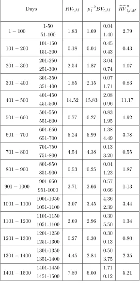
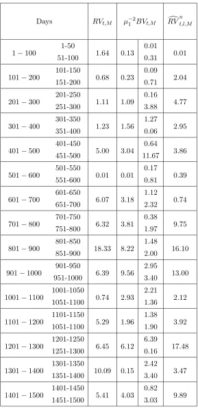
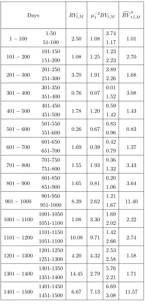
The square root model for the volatility component has been tested considering all the realized measures considered in Section 5. In particular, the test has been conducted for
(a) realized volatility, using a time span of a hundred days (T = 100) and an intradaily frequency
of five minutes (M = 79);
(b) normalized bipower variation, using two different daily time spans (T = 50,100), with M =
79;
(c) subsampled robust realized volatility, usingT = 100,M = 2341, the size of the blocks l= 30
and finally the number of blocksB = 78.
The results are summarized in Tables 1 to 3. The Tables reveal some interesting findings. First, it seems that the square root model is a good candidate to describe the dynamic behaviour of the volatility, at least in the chosen sample. In fact, especially for General Electric and Microsoft, the model is rejected only for a relatively small fraction of times, irrespective of the realized measure used.
bipower variation; this is a signal that in that period jumps have occurred in the log price process. For example, this happens for Intel for the periods going from day 701 to 800 and from day 1101 to 1200; for Microsoft, for the periods going from day 901 to 1000. Conversely, there are cases where the only measure which does not reject the model is modified subsampled realized volatility; this is a signal that in that period prices are strongly contaminated by microstructure effects. This happens for General Electric for the periods going from day 601 to 700 and 701 to 800; for Microsoft, for the periods going from day 1101 to 1200 and 1201 to 1300. The test using normalized bipower variation and conducted with T = 50, to conform to the regularity conditions in Proposition 2,
generally confirms the findings of the test with T = 100. Of course, in this case the power of the
test may be particularly low, due to smaller number of observations used.
Finally, it is worth mentioning the relative stability of the estimated parameters over different stocks and over different time spans. Specifically,µranges from 0.0003 and 0.0004,η from -0.02 to 0.05 andκ from 1 to 3.
7
Concluding Remarks
In this paper a testing procedure for the hypothesis of correct specification of the integrated volatil-ity process is proposed.
The procedure is derived by employing the flexible eigenfunction stochastic volatility model of Meddahi (2001), which embeds most of the stochastic volatility models employed in the empirical literature. The proposed tests rely on some recent results of Barndorff-Nielsen & Shephard (2001, 2002), ABM2002 and Meddahi (2003) establishing the moments and the autocorrelation structure of integrated volatility.
The tests are performed by comparing sample moments of realized measures with those of either the analytical moments of integrated volatility, when these are known, or with those of simulated integrated volatility. We provide primitive conditions on the measurement error between integrated volatility and realized measure, which allow to consider an asymptotically valid test for overidentifying restrictions. We then provide regularity conditions on the relative rate of growth of T, l, M under which realized volatility, normalized bipower variation and modified subsampled
realized volatility satisfy the given primitive conditions on the measurement error.