Addressing concerns in performance prediction : the impact of data dependencies and denormal arithmetic in scientific codes

(1)

University of Warwick institutional repository: http://go.warwick.ac.uk/wrap

A Thesis Submitted for the Degree of PhD at the University of Warwick

http://go.warwick.ac.uk/wrap/3713

This thesis is made available online and is protected by original copyright.

Please scroll down to view the document itself.

(2)

Addressing Concerns in Performance Prediction:

The Impact of Data Dependencies and Denormal

Arithmetic in Scientific Codes

by

Brian Patrick Foley

A thesis submitted to the University of Warwick in partial fulfilment of the requirements

for admission to the degree of

Doctor of Philosophy

Department of Computer Science

(3)

Abstract

To meet the increasing computational requirements of the scientific community, the use of parallel programming has become commonplace, and in recent years distributed applications running on clusters of computers have become the norm. Both parallel and distributed applications face the problem of predictive uncertainty and variations in runtime. Modern scientific applications have varying I/O, cache, and memory profiles that have significant and difficult to predict effects on their runtimes. Data-dependent sensitivities such as the costs of denormal floating point calculations introduce more variations in runtime, further hindering predictability. Applications with unpredictable performance or which have highly variable run-times can cause several problems. If the runtime of an application is unknown or varies widely, workflow schedulers cannot efficiently allocate them to compute nodes, leading to the under-utilisation of expensive resources. Similarly, a lack of accurate knowledge of the performance of an application on new hardware can lead to misguided procurement decisions. In heavily parallel applications, minor variations in runtime on individual nodes can have disproportionate effects on the overall application runtime. Even on a smaller scale, a lack of certainty about an application’s runtime can preclude its use in real-time or time-critical applications such as clinical diagnosis.

This thesis investigates two sources of data-dependent performance variability. The first source isalgorithmicand is seen in a state-of-the-art C++biomedical imaging application. It identifies the cause of the variability in the application and develops a means of characterising the variability. This ‘probe task’ based model is adapted for use with a workflow scheduler, and the scheduling improvements it brings are examined.

The second source of variability is more subtle as it ismicro-architecturalin nature. Depending on the input data, two runs of an application executing exactly the same sequence of instructions and with exactly the same memory access patterns can have large differences in runtime due to deficiencies in common hardware implementations of denormal arithmetic1. An exception-based profiler is written to detect occurrences of denormal arithmetic and it is shown how this is insufficient to isolate the sources of denormal arithmetic in an application. A novel tool based on the Valgrind binary instrumentation framework is developed which can trace the origins of denormal values and the frequency of their occurrence in an application’s data structures. This second tool is used to isolate and remove the cause of denormal arithmetic both from a simple numerical code, and then from a face recognition application.

(4)

Acknowledgements

Firstly I’d like to thank my supervisor Stephen Jarvis for overseeing my years at Warwick, and providing encouragement and guidance through academia and the world of High Performance Computing.

Thanks to Dan Spooner for many stimulating and varied discussions over the course of three years. A dozen papers could be written on the subjects discussed, and a small fortune spent on the shiny toys from Silicon Valley we examined.

Thanks to Paul Isitt for being an accommodating lab-mate, paper co-author and general collaborator as we explored the work of HPSG and the performance pre-diction community.

Thanks to Russell Boyatt for providing much useful technical advice, many movie recommendations, and for being an obliging sounding board.

(5)

This thesis is dedicated in loving memory of my father, 1952–2009

(6)

Declarations

This thesis is presented in accordance with the regulations for the degree of Doctor of Philosophy. It has been composed by myself and has not been submitted in any previous application for any degree. The work described in this thesis has been undertaken by myself except where otherwise stated.

The following publications relate to the thesis text:

• _{Brian P. Foley, Paul J. Isitt, Daniel P. Spooner, Stephen A. Jarvis, and Graham}

R. Nudd. Implementing Performance Services in Globus Toolkit v3. In Proceed-ings of the UK Performance Engineering Workshop, July 2–8 2004, Bradford, UK.

[Appendix B]

• _{Brian P. Foley, Daniel P. Spooner, Paul J. Isitt, Stephen A. Jarvis, and Graham}

R. Nudd. Performance Prediction for a Code with Data-dependent Runtimes. Awarded best paper at UK eScience All Hands Meeting, September 19–22 2005, Nottingham, UK.[Chapter 3]

• _{Stephen A. Jarvis, Daniel P. Spooner, Brian P. Foley, Paul J. Isitt, Graham R. Nudd.}

Predictive Workflow Scheduling for Multi-Clusters and Grids. CORS/INFORMS Joint International Meeting, May 16–19 2004, Banff, Alberta, Canada. [Chapter 3] • _{Paul J. Isitt, Stephen A. Jarvis, Brian P. Foley, Daniel P. Spooner, and Graham}

R. Nudd. Towards Performance-aware Real-time Management for On-demand Computing Environments. In the 7th International Workshop on Performability Modeling of Computer and Communication Systems (PMCCS), September 23–24 2005, Torino, Italy. [Chapter 3]

• _{Stephen A. Jarvis, Brian P. Foley, Paul J. Isitt, Daniel R ¨uckert, and Graham R.}

Nudd. Performance Prediction for a Code with Data-dependent Runtimes. In Concurrency and Computation: Practice and Experience19:1–12, 2007. [Chapter 3] • _{Brian P. Foley, and Stephen A. Jarvis. Tracing Denormal Arithmetic with Valgrind.}

Submitted to the37th_{International Symposium Computer Architecture (ISCA 2010),} June 19–23, Saint Malo, France. [Sec. 5],[Chapter 6]

(7)

List of Tables

3.1 EvaluateGradientiterations . . . 47

3.2 EvaluateDerivativecosts . . . 49

3.3 Parallel speedup ofnregvs sequential code . . . 49

3.4 Comparing scheduling techniques with varying workloads. . . 60

3.5 The effect of probe task speed on makespan . . . 61

4.1 Single-precision storage in IEEE-754 . . . 72

4.2 Flush to zero behaviour . . . 73

4.3 Gradual underflow with denormals . . . 73

4.4 Divide by zero without denormals . . . 74

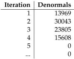
4.5 Denormals at cfd-sor startup . . . 84

4.6 Denormal instruction profile in cfd-sor . . . 86

6.1 fval info table for a simple expression . . . 127

6.2 Denormal exception profile forjacobi . . . 131

6.3 DART denormal profile forjacobi . . . 132

6.4 Denormal loads/stores forjacobiarrays . . . 134

6.5 Denormal exception profile for187.facerec . . . 137

6.6 DART denormal profile summary for187.facerec . . . 138

6.7 Denormal array accesses in187.facerec . . . 141

6.8 Denormal origins in187.facerec. . . 144

6.9 Genuine denormal origins in187.facerec . . . 147

6.10 Genuine denormal array accesses in187.facerec . . . 147

6.11 Denormal exception profile for patched187.facerec . . . 148

6.12 Denormal array accesses in patched187.facerec . . . 148

6.13 DART denormal profile for patched187.facerec . . . 150

A.1 5 bit unsigned minifloat values . . . 158

F.1 DART denormal profile for187.facerec, part I. . . 177

F.2 DART denormal profile for187.facerec, part II . . . 178

F.3 DART denormal profile for187.facerec, part III. . . 179

G.1 Comparing scheduling techniques with varying workloads . . . 180

(12)

(13)

List of Figures

1.1 Data hazard in a Central Processing Unit (CPU) with a 3 stage pipeline 3

1.2 Register renaming used to avoid anti-dependency ofI3onI1. . . 6

2.1 NWS clique hierarchy . . . 28

2.2 LDAP object class . . . 29

2.3 LDAP distinguished name . . . 29

2.4 Sweep3D wavefront behaviour . . . 31

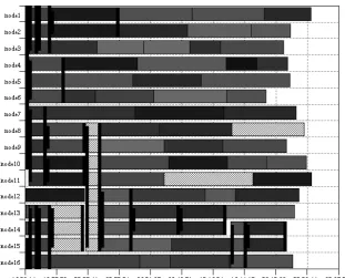
2.5 Run-time schedule of three example workflows. . . 38

3.1 Slices from brain scans in need of registration . . . 43

3.2 Transformation of 2-D image bynreg . . . 44

3.3 Runtime variation for different images . . . 50

3.4 Runtime scaling with subsampled images . . . 52

3.5 Predicted runtimes . . . 53

3.6 Prediction error . . . 53

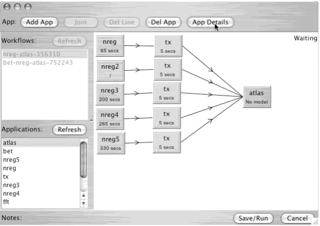
3.7 Operation of the performance-aware resource management system . 54 3.8 Workflow builder with performance model evaluation . . . 56

3.9 Workflow scheduling a mix of speculative and real tasks . . . 58

4.1 A 5 bit ‘minifloat’ format . . . 69

4.2 IEEE-754 float and double formats . . . 71

4.3 jacobiinner loop . . . 78

4.4 Compiled code . . . 78

4.5 Linux FPE handling . . . 83

4.6 K´arm´an vortex sheet incfd-sor . . . 84

5.1 Valgrind instrumentation process . . . 90

5.2 Heap overflow. . . 93

5.3 Use afterfreeerror . . . 93

5.4 Invalid data propagation . . . 94

5.5 Linux 2.6.x x86 memory map . . . 101

5.6 Dynamic and compile time allocation . . . 104

5.7 Two level tag table . . . 107

(14)

5.9 Trace log from an examplejacobikernel . . . 113

5.10 Graph of operations from an examplejacobikernel . . . 114

5.11 Multi-copy code . . . 114

5.12 Trace log of multi-copy code . . . 114

5.13 Graph of multi-copy code operations . . . 115

6.1 Laplace steady state approximation afterNiterations . . . 119

6.2 187.facereclocal frequency measurements[PKvdM96] . . . 120

6.3 Distinct tables for tag and read/write counts. . . 124

6.4 Tags for a simple expression . . . 127

6.5 jacobikernel instructions . . . 130

6.6 Heatmap showing sweep of denormal averages produced byjacobi 135 6.7 Map of number of denormals injacobiarrayaderived fromb. . . . 136

6.8 Array elements with denormal values in the five187.facereckernels.142 6.9 187.facerectemporary array denormal heatmaps. . . 143

6.10 187.facerecorigin maps . . . 145

A.1 5 bit minifloat compared to IEEE-754 float . . . 157

A.2 A 5 bit ‘minifloat’ format . . . 158

B.1 Excerpts from theSunUltra 10.hmclhardware model. . . 159

B.2 Theasync.laparallel template . . . 160

B.3 blend.c. . . 160

B.4 blend.la– the blend subtask . . . 161

B.5 blend app.la– the application model . . . 161

(15)

Abbreviations

ALU Arithmetic and Logic Unit

CHIP3S Characterisation Instrumentation for Performance Prediction of Parallel Systems

CPU Central Processing Unit

CTMC Continuous Time Markov Chain

DAG Directed Acyclic Graph

DIE Debugging Information Entry

DIT Directory Information Tree

DN Distinguished Name

FIFO First-In First-Out

FPU Floating Point Unit

GIIS Grid Index Information Service

GLUE Grid Laboratory Uniform Environment

GRAM Grid Resource Allocation Manager

GRIP Grid Information Protocol

GRIS Grid Resource Information Service

GRRP Grid Registration Protocol

IDT Interrupt Descriptor Table

IPC Instructions Per Clock

IR Intermediate Representation

(16)

LDAP Lightweight Directory Access Protocol

LU Least Upper matrix decomposition

MDS Monitoring and Discovery Service

MMU Memory Management Unit

MPI Message Passing Interface

NWS Network Weather System

ODE Ordinary Differential Equation

OGSI Open Grid Services Infrastructure

PACE Performance Analysis and Characterisation Environment

PEPA Performance Evaluation Process Algebra

QoS Quality of Service

RTL Register Transfer Language

SMT Simultaneous Multithreading

SOAP Simple Object Access Protocol

TLB Translation Lookaside Buffer

WSRF WS-Resource Framework

iFFT Inverse Fast Fourier Transform

(17)

(18)

CHAPTER

1

Introduction

From the invention of the first electronic computers to the sophisticated systems of today, the increase in available processing power has been enormous. Cambridge University’s EDSAC, a typical early computer, had approximately 500 words of memory and could execute 600 instructions per second [CK92]. In 2009, an inex-pensive laptop is likely to have more than a million times as much memory and several million times as much processing power; and a high end cluster can provide more than 10,000 times as much usable compute power again.

The availability of large amounts of inexpensive processing power has enabled the mathematical and scientific communities to perform research that would other-wise have been impossible. Despite this continual growth, the demand for more processing power than is readily available has remained constant. von Hoerner’s stellar dynamics simulations in 1960 modelled systems with about 16 particles; the current equivalents are cosmological models with 109 particles [vH60, TCPP98]. Protein folding [Pan02], medical image processing and number theory [Wol96] are examples of the many scientific domains that absorb as muchCPUtime and storage as can be provided.

Until recently, Moore’s law1 has provided continual increases in inexpensive se-quential compute performance, but there are warning signs that this exponential growth is becoming difficult to sustain.

1.1 CPU performance prediction

For decades, single-threaded microprocessor performance has benefited from Moore’s Law. Due to the relatively large transistor size, and limited die area on a silicon chip, early microprocessor designs had very limited transistor budgets, and were forced to have few registers, to omit any non-essential functionality, and to implement critical components such as Arithmetic and Logic Units (ALUs) and control units using as few transistors as possible. One way of doing this is to operate on the data serially2or a few bits at a time. The downside of this approach is that to perform a 1_{An empirical observation that the number of components that can be fitted on a given area of} silicon at a given price point seems to double approximately every 18 months

(19)

single operation, pieces of a word of data have to pass through theALUin several stages, increasing the number of clock cycles taken to perform the operation. As the transistor budget increased, widening the data paths and expanding theALU was one obvious way to improve performance. When data paths become fully parallel, further performance improvements were achieved by reducing the depth of the logic trees required to implement operations such as add and multiply. This was done at the cost of extra transistors using techniques such as carry look-ahead blocks for adders and Wallace trees [Wal64] for multipliers.

As the transistor size decreased and transistor budget increased, performance rapidly increased along with it. Some of these improvements included:

• _{Both the amount of time and the power needed to switch a transistor on and o}ff

decreased, leading to an increased clock rate.

• _{ALUs became fully parallel, allowing additions, e}ff_{ective address calculations,}

and program counter updates to be performed in one clock cycle.

• _{Hardware multipliers could be implemented, first in serial-parallel form, and}

later fully parallel. This was accompanied by hardware dividers, although with less parallelism. Early multipliers and dividers typically generated one or two bits of output per clock cycle.

• _{When the transistor budget reached a certain threshold, floating point co-processors}

became practical, and later benefited from increasingly parallel implementations.

• _{Eventually Floating Point Unit (FPU) co-processors were integrated on the same}

chip as theCPU. This reduced the communications overhead between theCPU andFPU, further improving performance.

Although these advancements dramatically improvedCPU speed, the behaviour of a CPU still remained relatively predictable and straightforward, and none of these advances causes substantial difficulties for performance estimation techniques based on simple instruction counting.

During the early to mid 1990s however, processor manufacturers started to include features that yielded substantial performance improvements, but would prove much more challenging to model. Techniques included:

• _{Functional units on}_{CPUs started to become heavily pipelined. So, for example,}

(20)

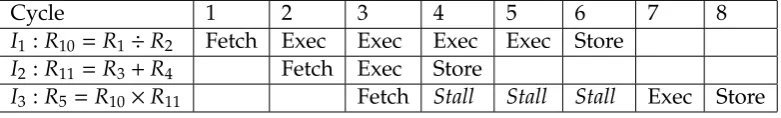
Cycle 1 2 3 4 5 6 7 8 I1:R10=R1÷R2 Fetch Exec Exec Exec Exec Store

I2:R11=R3+R4 Fetch Exec Store

[image:20.595.101.492.108.167.2]

I3:R5=R10×R11 Fetch Stall Stall Stall Exec Store

Fig. 1.1: Data hazard in a CPU with a 3 stage pipeline where divides have a 4 cycle latency. The third instruction cannot execute until after the two previous instructions have stored their results.

one stage of a 7 stage pipeline. However, once the first stage had completed, it became available for use by another instruction. One divide would take 7 clock cycles to complete, but 100 independent divides one after the other would only take 107 cycles to complete. Pipelining can be very effective, but fails to deliver a performance benefit when subsequent instructions depend on the results of an earlier instruction that is still going through a pipeline. When this happens the pipeline ‘stalls’ — theCPUmust wait for the first instruction to complete before the second instruction can be issued. To model this, performance estimation software has to know the depth of each of the pipelines in theCPU, and track the dependencies between instructions. Fortunately this can be accurately modelled solely by static analysis of the instruction stream itself. A simple example can be seen inFig. 1.1.

• _{Memory Management Units (MMUs) and memory caches began to be integrated}

on chip, and moved from direct mapped to more efficient and complex set-associative schemes reducing the need to access slow main memory. This had the benefit of decreasing the average amount of time a CPU had to wait to read/write memory, improving performance. However introducing extra layers into the memory hierarchy meant that memory access times were no longer constant. Two pieces of code with exactly the same mix of instructions could run at dramatically different speeds depending on whether their memory access patterns were cache-friendly or not. Unlike pipelining, cache behaviour is not readily amenable to static code analysis, and this causes considerable problems for performance estimation, although it is possible to apply heuristics to estimate the effects of some common memory access patterns [Har99].

(21)

at a considerable cost. If the program’s memory access patterns touches many pages of memory, the TLB thrashingthis causes can be a significant slowdown. As with memory cache performance analysis, this cannot be analysed statically, but similar heuristics can be applied; MMUpages in aTLBwill have a similar eviction policy to cache lines in a memory cache.

• _{To reduce the impact of the pipeline stalling problems mentioned above,} _CPUs

started to use more sophisticated control units to allow ‘Out-of-order Execution’. Rather than issuing instructions strictly in order, theCPUqueues up a number of instructions for execution. When the operands for that instruction become available and a functional unit is not busy, the instruction is issued for execution on that unit. As instructions complete, their results are retired, or queued for writing to the appropriate registers. Thus, a single instruction with a dependency will no longer stall the pipelines of all the functional units until the dependency is met. Instead the instruction itself will be delayed and other instructions are free to be issued ahead of it as long as they don’t depend on any unavailable results.

To make this more effective, Out-of-Order CPUs tend to have large numbers of rename registers as well as multiple copies of functional units which are not directly visible to the programmer. The net effect of Out-of-Order execution is to allow a serial instruction stream with possible pipeline-stalling dependencies to be translated into a parallel stream of instructions, one stream per functional unit. When this works, aCPUcan issue and retire several instructions per clock cycle, although in practice significant amounts of parallelism are difficult to achieve. Also, this makes life especially difficult for performance estimation software, as it now has to deal with an instruction stream which may be translated into several different instruction streams in a different order. Worse still, the streams can have interdependencies, and the same piece of code in memory may be translated into a differently ordered stream and issued to different units every time it is encountered depending on the internal state of each of functional units in the CPU. To determine the cost of an instruction, its overallcontextand the internal state of the CPU are far more important than the actual instruction itself. A simple example of register renaming can be seen inFig. 1.2.

• _{A final set of techniques that modern}_{CPUs use to try to alleviate pipeline stalls}

(22)

instruc-tions until a branch’s arguments are known, and to only continue after that. This causes serious pipeline stalls however, and since branch instructions are common, it causes a major performance penalty. To deal with this, Out-of-OrderCPUs can guess which direction a branch is going to proceed, speculatively execute beyond the branch instruction, and store the results of speculative instructions to tempo-rary registers. When the branch dependencies are finally resolved, if the guess was incorrect, the unneeded computations are discarded. If the guess is correct the results in the temporary registers are retired. If enough functional units and rename registers are available, theCPUcan speculatively executebothpaths of a branch, and discard the unnecessary one when the branch dependency becomes available.

Of course, if the branch prediction is unsuccessful, it causes unnecessary in-structions to be issued, but as long as it is correct some of the time, it is still a performance benefit, as it allows some use to be made of otherwise idle execution units.

To improve the impact of speculative execution, modern CPUs maintain large tables of statistics describing which direction a particular branch instruction is likely to go. As each branch is taken or not, the statistics are updated, and thus theCPU builds up a model of the branch behaviour of the program. As with Out-of-order Execution, the internal state of theCPU, or more specifically of the branch prediction tables determines the cost of the instruction. Other than in simple cases, the probability of following a branch is related to the input data, and so, unlike Out-of-order techniques, the effectiveness of branch prediction is dependent on the program data itself. This is something that it is impossible for performance modelling software to analyse statically, and poses another problem for performance prediction systems like PACE [NKP+00]. Other systems, such as Prophesy and WARPP sidestep this problem by relying on coarser grained benchmarks for the basic blocks in an application.

The above techniques have all been inspired by the continually increasing transistor budget and a desire to extract as much parallelism as possible from a sequential instruction stream, but they come at a cost. In particular, aggressive speculative execution yields a linear increase in Instructions Per Clock (IPC) rates for an expo-nential cost in transistors, design complexity, and power consumption.

(23)

Without register renaming.

Cycle 1 2 3 4 5 6 7 8 10 11 12 13 14

I1:R1=R10÷R11 IF EX EX EX ST

I2:MEM(1000)=R1 IF - - - EX ST

I3:R1=R12÷R13 IF - - - - EX EX EX ST

I4:MEM(1001)=R1 IF - - - EX ST

With register renaming.

Cycle 1 2 3 4 5 6 7 8 10 11 12 13 14

I1:R1a=R10÷R11 IF EX EX EX ST

I2:MEM(1000)=R1a IF - - - EX ST

I3:R1b=R12÷R13 IF EX EX EX ST

I4:MEM(1001)=R1b IF - - - EX ST

Fig. 1.2: Register renaming used to avoid anti-dependency ofI3onI1.

Bor03]. As a result of this, the industry has moved away from scaling clock speeds and using aggressive speculative execution to speed up sequential codes. Instead the emphasis is now on making more efficient use of the growing transistor budget constrained by a fixed power budget by providing several less aggressive CPU cores on the one die, each running independent instruction streams. Commercial examples of this include Intel’s Core family ofCPUs, IBM’s POWER series, and Sun’s recent UltraSPARCs. The same trends are driving the performance of graph-ics processing units capable of restricted forms of computation, and digital signal processors. Graphics processing units can take advantage of a more constrained computational model than general purposeCPUs and so have a much higher pro-portion of their transistors allocated toFPUs instead of control logic. This makes them significantly faster than general purposeCPUs for applications that fit their computational restrictions.

(24)

1.2 Context and Previous Research

The High Performance Systems Group at the University of Warwick have demon-strated that performance prediction, i.e., the rapid estimation of the resource usage of an application on a given computer, is essential for the efficient utilisation of distributed systems. [JSK+06]

Under previous research, techniques and tools have been developed at Warwick such as the Performance Analysis and Characterisation Environment (PACE) [NKP+00] toolkit. PACE uses a combination of static code analysis, micro-benchmarking and event simulation to rapidly provide runtime estimations of performance and for both sequential and distributed applications [CKPN99], and has been used in ap-plication steering and job scheduling systems [KPN98,SJC+03].

Another researcher, also at Warwick, developed a scheduler called TITAN [SJC+03] which has shown that significant performance improvements can be achieved by using performance models as part of performance-responsive middleware services that address the implications of executing a particular workload on a given set of resources.

Since PACE was developed, both scientific applications and the hardware that they run on have increased in complexity. Binary compatibility means that old applications will generally run on new hardware; but due to architectural changes, code sequences which may have been optimal on an older processor might perform poorly on a more recent one. Performance prediction becomes much more difficult for the reasons mentioned above, and in these new environments, the speed at which a fragment of code executes now depends largely on its context, i.e., the state of theCPU and the mix of instructions and memory accesses used and not the individual instructions. Context, in turn is determined by the flow of control within an application, and for all but deliberately regular applications, the flow of control depends on the input data.

(25)

allocation of copy-on-write objects as they are modified and more.

Concurrently with the work in this thesis, another PACE-like tool called WARPP is under development by a different set of research students at Warwick. WARPP, which discussed in more detail inSec. 2.1.3avoids some of the issues of application complexity and code context by basing itsCPUsimulations on benchmarks of the basic blocks of an application on the target hardware. Research is underway to automate the instrumentation and benchmarking process as much as possible. By their nature, these benchmarks only measure the average case and will not, for example, capture variability due to unpredictable memory access patterns or other data-dependent effects.

1.3 Thesis Contributions

These factors when taken together make it increasingly difficult to build perfor-mance models based solely on static code analysis and benchmarks — whether coarse or fine grained. This thesis explores this notion of data dependency. The term data dependency has multiple meanings — from the dependencies between in flight instructions in a CPU; to the abstract graph of computations that a compiler manipulates; to the relationship between groups of communicating processes. The meaning here is distinct from, but related to the first two: it refers to the notion that when the information content of an application’s input data changes, the perfor-mance of the application can change unexpectedly too. This can be simply because the different data makes an algorithm perform more work, by iterating more, or by using different code paths; or it can be because the different data triggers certain hardware behaviours.

To do this, I examine two types of application. The first is a medical imaging application with highly variable runtimes. These variations are caused by the application’s algorithms themselves, in part because of their convergence criteria, but also because of how the application samples its datasets. I build a performance model for this heretofore unpredictable application based on the application’s input data. This model requires some pre-executionCPUtime for every task it models, and I adapt TITAN to accommodate this and to use the sequence of increasingly refined predictions it emits.

(26)

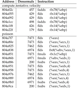
larger than zero. These numbers have a different representation to normal num-bers, and require special handling by the floating point implementation. I describe a simple means of detecting denormal arithmetic and show its limitations. Based on this, I build a more sophisticated tool to track denormal data in an application back to its origins. This origin tracking aids the developer in eliminating denor-mal arithmetic in an application producing a faster, but more importantly, more predictable application.

The primary contributions of this work are as follows:

• _{Developing a performance model for a state-of-the-art C}++_{medical imaging}

application. Initial attempts to build a PACE-based performance model for this application, nreg, failed for two reasons. Firstly,nreg makes pervasive use of inheritance and C++ templates and needs compiler optimisations to run effi -ciently, neither of which PACE could handle. Furthermore, the application itself exhibits data-dependent runtime variability, i.e., two input datasets of exactly the same size can easily have more than an order of magnitude difference in runtime. PACE could only provide predictions for the average case, which are of little use in this situation. I develop an alternate data-driven model which makes it possible to estimate the runtime ofnreg. This makes it possible to usenregin scenarios where quality of service criteria are useful, such as in clinical diagnosis, or to allow efficient task scheduling.

• _{Analysing how computationally intensive performance prediction processes}

may be used as a part of a scheduler. As part of its scheduling algorithm, TITAN makes the assumption that performance data for its applications are available at negligible cost, and makes many queries to the prediction engine for every iteration of its genetic algorithm. The performance model fornreg takes some time to evaluate, and the moreCPUresources given to the performance model, the more accurate the prediction. These performance prediction ‘probe tasks’ need to be run on the same compute resources as the actual tasks, and thus need to be scheduled along with them. I modify TITAN to do this, and analyse the effects the asynchronous stream of continually improving predictions have on scheduling quality, and how it may be used for ‘interactive scheduling’.

• _{Profiling application runtime variability caused by denormal arithmetic}_{. Many}

(27)

in recent Intel x86 processors. To measure the occurrence of denormal arith-metic, I write and use a floating point exception based profiling tool called DIP. I show why profiling is insufficient to identify the true sources of performance degradation.

• _{Finding the origins of denormal arithmetic and removing it from an application}

using a novel tool. The dynamic binary instrumentation framework Valgrind [NS07b] is described, and using its facilities, I write DART, a denormal arithmetic tracing tool. I implement three different methods for analysing the information gathered by DART. I then use DIP and DART to examine the flow of denormal data in the two numerical codes. The sources of the denormal data are found and eliminated, producing more predictable applications as a result.

1.4 Thesis Overview

The thesis is divided into 7 chapters. The remaining chapters are organised in the following fashion:

Chapter 2 Existing performance prediction techniques are reviewed, an existing analytical performance model is examined, and the iterative heuristic sched-uler TITAN is described.

Chapter 3 The medical imaging application nreg is analysed, and a novel data-driven performance model is developed for it. The chapter describes how a continually improving series of performance predictions over time can be integrated into a workflow scheduler. It shows how this can provide per-formance information to the user and using this as a part of an ‘interactive scheduling’ process.

Chapter 4 The IEEE-754 Floating point arithmetic standard is described, with an emphasis on the performance aspects of denormal arithmetic and common hardware implementations. DIP, a profiling tool based on floating point exceptions is written, and its limitations are examined.

(28)

Chapter 6 DIP and DART are used to analyse the behaviour of two applications. The sources of denormals are identified and removed from both applications, thus removing a source of performance variability. Limitations of DART are discussed.

(29)

(30)

CHAPTER

2

Performance prediction and its application

Performance prediction for high performance computing involves two separate phases. The first gathers performance data for the compute resources in question, and the second uses the data as part of a performance model.

Performance data is typically gathered using some sort of benchmarking or per-formance measuring technique. Since hardware failures are common in systems with large numbers of components, and failure is often preceded by performance degradation, it is common to integrate this into a cluster monitoring system rather than simply benchmarking the system once. On task completion, basic statistics are often recorded too, such as the overall runtime, number ofCPUs used, and the working set of the tasks. The data gathered is then stored in some sort of repository where it can be queried and analysed.

Performance modelling of the applications themselves is the second stage of predic-tion. These models can be as simple as an averaging of the runtimes recorded by the performance monitoring system, or may include complex analytical models such as those to be described inSec. 2.3. Irrespective of the complexity, these performance models use the performance characteristics of the hardware as parameters, and so cannot generate performance predictions in isolation.

A major use for these performance prediction models is in resource allocation systems, such as job schedulers; in middleware for instantiating abstract workflows; in parallel applications which try to balance their workload across multipleCPUs; and in performance models used to guide hardware procurement by estimating application scalability on hypothetical systems. Performance prediction can also be useful when trying to determine why an application does not perform as well as expected on a new system [PKP03].

(31)

2.1 Performance modelling tools

Depending on the problem domain, a whole spectrum of performance measure-ment and modelling techniques can be used. These vary in sophistication: Simple techniques use black box timings of a set of candidate workloads as the measure-ment, and curve fitting as the model; more sophisticated approaches gather sets of hardware microbenchmarks and feed them to application models of what compu-tations are performed and how they are distributed across a cluster.

The more sophisticated models usually have the benefit of having more explana-tory power, and providing more reliable predictions; however they are also more difficult to create, rely on a deeper understanding of the hardware and software, and may be slow to evaluate.

Another approach is to model software systems in a more abstract and mathematical manner by treating them as a set of interacting components specified using a formal language. When specified in this way, numerical and analytical tools can be used to find solutions to the steady state performance of the system.

2.1.1 SimpleScalar

Due to the complexities of modern microprocessors mentioned in Sec. 1.1 there are many challenges to predicting the performance of a piece of code on a given processor. The most direct way to solve this problem is to exactly simulate each component of the processor’s micro-architecture and to run the code directly on the simulation—or feed an instruction trace into it—and observe the results of the simulation. Tools such as SimpleScalar [BA97] do exactly this, and because of the precision of their results they are mostly used during the design of microproces-sors. Because of the fact that they have to fully model the behaviour of the cache hierarchy, the functional units, the logic associated with Out-of-order Execution and maintain profiling information for all of these, simulators of this sort run much slower than native hardware. For example, the most detailed SimpleScalar 2.0 sim-ulator running on a machine capable of more than 200 MIPS executes approximately 150,000 simulated instructions per second, a factor of more than 1,000 slowdown. SimpleScalar 4 has a similar slowdown: a full simulation on a 1.6 GHz Pentium 4 system runs at 350,000 IPS.

(32)

benchmark application kernels on hypothetical systems, and these benchmarks can be used together with other less detailed performance modelling tools.

Because of their accuracy, these tools can also be useful both for low-level tun-ing of application kernels on a specific micro-architecture, and for designtun-ing new processors that work better with common workloads. One instance of this is the tool WATTCH [BTM00] built on top of SimpleScalar which predicts the power con-sumption of a processor under particular workloads. It does this by modelling the power draw of different primitive units within the processor (such as clocks, busses, logic, and memory arrays) and describes each part of the processor (such asTLBs or branch prediction units) in terms of these. When an instruction stream runs on the processor, the approximate number of transistor switchings in each unit is measured, and from this the overall power draw can be calculated.

2.1.2 PACE

PACE, the Performance Analysis and Characterisation Environment [NKP+00] was developed by the High Performance Systems Group at the University of Warwick in the late 1990s and early 2000s to predict the runtime and resource usage of scientific applications using pre-execution modelling and analysis. PACE provides rapid and accurate estimations for both sequential and distributed applications [CKPN99], and has been used in application steering and job scheduling systems [KPN98,SJC+03].

Rather than directly simulating the execution of a code-base as micro-architectural simulators do, PACE uses a language called Characterisation Instrumentation for Performance Prediction of Parallel Systems (CHIP3_{S) to build a static performance}

model of an application program. This language provides constructs to describe the flow control, overall instruction usage and communications patterns of an application in a parameterised fashion. PACE includes facilities to benchmark computation and network performance on a candidate hardware platform, and allows the application models to be evaluated against these hardware models. CHIP3_S_{performance scripts, written using a C-like syntax, are compiled and linked}

(33)

PACE’s application models decompose into a set of subtasks, which in turn can contain other subtasks. Each subtask in CHIP3_S _{consists of a sequence of flow}

control elements (bounded loops, and conditional statements) and each element (or block) contains a number of primitive operations. These primitive operations are characterised by a fixed delay and include such events as floating point mul-tiplies, memory accesses and array indexing. Interprocess communications via Message Passing Interface (MPI) are characterised using a network model based on bandwidth and latency. The characterisation models the fact that small MPI messages have different performance characteristics to largeMPImessages in most implementations.

The hardware models contain a list of costs (or characterisations) of each primitive operation for a given hardware architecture, and the file format PACE uses for hardware models is modular and extensible. Early PACE hardware models only had characterisations for instruction sequences used in C programs. Over time, various projects extended this to include characterisations for processor caches, and the memory hierarchy [Har99]; inter-node communications via MPI, MI and PVM; performance of SUIF primitives [WFW93]; and the cost of interpreting Java bytecodes [Tur03].

The final component in a PACE application model is the parallel template. This pro-vides a means of expressing the costs and constraints associated with subdividing a task to run on multiple processors in a cluster. Applications withinCHIP3Sare eventually decomposed to blocks of primitive compute operations interleaved with communications. PACE’s parallel templates have astepdeclaration which refers to a block of computation within a subtask, and statements indicating communication between two nodes.

The blocks from each of the subtasks are taken and compiled into a control flow of blocks. When run, each of these subtasks and each synchronous block is eval-uated according to the model scripts and a predictive trace is made of operation usage. This is then translated into resource usage using the data from a hardware model. When communications occur they introduce dependencies betweenCPUs, and a simple discrete event simulation is used to order the communications and computations on a time line.

(34)

costs of network communication well, and in practice these contribute to a large portion of the runtime of typical parallel scientific applications.

A simple performance model is described in more detail inAppendix B.

2.1.3 WARPP

Although successful in modelling some classes of applications, PACE’s reliance on models derived from the source code of the application rather than from the opti-mised binaries produced by a compiler has become more and more of a problem. As discussed previously, modern processors are extremely complex internally and rely on sophisticated compiler techniques to schedule instructions, allocate regis-ters, unroll loops etc. so that the best use is made of the processor’s functional units and cache. PACE’s assumption that a C construct such as a single iteration of loop or an array assignment can be characterised by a single timing is simply no longer true.

To deal with this problem and others, a new performance modelling framework called WARPP has been developed at Warwick [HMS+09] concurrently with the research in this thesis, but by different researchers. At a high level it is similar to PACE: parametric performance models for an application are written in a C-like scripting language. When executed, the models generates a trace of computation and communication events on all of the simulated CPUs which are fed into a discrete event simulator. A hardware model for both the network andCPUs orders assigns a timing to each event, and the simulator uses these timings to order the communications and computations on a timeline.

The differences lie in the details:

• _PACE’s_CPU_{models are based on extremely fine grained microbenchmarks, but}

they do not accurately capture the behaviour either of modern compilers or modernCPUs. To avoid the problem ofcontextmentioned inChapter 1, WARPP abandons fine grained microbenchmarks in favour of benchmarking each basic block of the application via compile time instrumentation.

• _{Like PACE, WARPP includes a model for network communications and for}

(35)

small and large messages as different regions. WARPP’s method is more flexible, allowing for multiple timings depending on the message size.

• _{WARPP allows a complex heterogenous network layout to be specified on a}_CPU

by CPU basis, for example extremely fast low latency IPC between CPUs on multicore chips, slower communications betweenCPUs on SMP compute nodes, and a system-wide interconnect between nodes. PACE simply assumes a flat, homogenous network topology.

• _{WARPP allows multiple}_CPU_{types to be specified in a system, each with its own}

set of benchmark measurements. PACE assumes a cluster of identicalCPUs.

• _{WARPP allows disc I}/_{O to be characterised, whereas PACE only models network}

I/O andCPU.

• _{WARPP and PACE use a similar discrete event system to schedule network}

events and thus calculate the delays associated with communications, however WARPP’s implementation is much more efficient, and scales effectively to very large numbers of CPUs. Initial attempts at a PACE performance model for Sweep3D as described in [MVJ08] had unacceptable runtimes and impractical memory usage for relatively small numbers ofCPUs.

Furthermore, experimental work has been done with WARPP to model performance variability in the form of ‘system noise’, or random occurrences of low-level slow-downs that frequently occur on cluster systems [HMS+09]. These can be caused by interrupt handlers, by network contention, or by system daemons running in the background that periodically wake up and perform a small amount of work. Regardless of the cause, system noise can have an effect on application runtimes hugely out of proportion with the individual slowdowns caused on each node [PKP03]. Initial experiments that inject compute noise into a running model exhibit similar slowdowns to those seen in a 960CPU commodity cluster in production use.

(36)

of a hand-generated model, they are much faster to create, and can later be tuned by hand for further accuracy.

2.1.4 Prophesy

The Prophesy system[TWL+01,TWS03] takes another high-level approach to mod-elling applications. Similar to PACE, it does not simulate individual instructions, but relies on higher-level abstractions. Instead of PACE’s modelling language, it relies on the notion that many applications can be decomposed into a set of kernels which consume most of the application’s runtime. If the performance character-istics of these kernels can be captured, and the kernels’ interactions when run together can be described, then it is possible to build up a performance model of entire applications without needing to analyse individual instructions.

Prophesy provides three connected components.

The first component is PAIDE, the Prophesy Automatic Instrumentation and Data Entry system.[WTS01] This is the ‘data gathering’ part of Prophesy. It automatically instruments source code on one of several levels: on the level of entire functions, entire loops, or even individual basic blocks. The instrumentation design min-imises overhead, and critical kernels or optimisation sensitive sections code can be instrumented less aggressively than the rest of the application. At runtime, the timings gathered by the instrumentation are sent to another Prophesy component along with a call graph of the application’s execution.

This information is placed into a performance database, the second component of Prophesy. The database has a hierarchical structure reflecting that of the appli-cation: an application is assumed to consist of a group of modules, each in turn subdivided into functions composed of basic blocks. The performance informa-tion about an individual execuinforma-tion of an applicainforma-tion (and its sub-components), the system it ran on, and the set of inputs used are stored in the database. Systems infor-mation includes the processor architecture, memory subsystem, operating system and network connections.

The final part of Prophesy is the modelling component. Here, individual kernels are modelled, and then composed to model the entire application.

(37)

method of least squares. Since this is a ‘black box’ approach, it is of limited utility: it cannot predict how a kernel will run on different hardware configurations, because it cannot know how a kernel depends on different performance characteristics of the hardware (e.g., one function might be sensitive to memory bandwidth, another to memory latency, and a third to the speed of floating point divides). Also, if the kernel or application has many input parameters, a large number of data points may be required to produce a model. However, in its favour, the technique is simple and may be useful for examining the scalability of some applications.

The second form of modelling requires the developer to use performance measure-ments along with manual analysis to create an equation describing the runtime of an application kernel in terms of the input and the hardware system. This analysis is difficult and time consuming, but need only be done once. For example, by inspecting a function, the programmer might see that a function makes

√

nlinear sweeps over an array of sizen2 and characterise the runtime in terms of memory bandwidth and array size.

The most novel feature that Prophesy introduces is that ofkernel coupling.[TWGS02] This describes the effect that running one kernel will have on runtime of another kernel that executes directly after the first. It is expressed as a ratio of the runtime of kernels executed in isolation vs the kernels executed together, or ifPiis the runtime of kernel running alone, andPi jis the runtime of two kernels running consecutively, Ci j, the coupling factor is

Ci j = Pi j Pi+Pj

For example, kernels Ki and Kj might use similar datasets, and because Ki has ‘warmed the caches’ forKjthe runtime ofKifollowed byKjmight be less than the sum of their runtimes in isolation, i.e.,Ci j<1. ConverselyKiandKjmight compete for resources andKimight force data used byKjout of main memory, requiringKj to page it back in when it runs. In this caseCi j>1. These two scenarios are called ‘constructive coupling’, and ‘destructive coupling’.

Kernels often occur in chains and loops, and Prophesy can use the information gathered for the coupling between individual pairs of kernels to predict the overall performance of an application. It was found in [TWGS02] that predictors using kernel coupling give much more accurate performance estimates than those based simply on summing the runtimes of each kernel.

(38)

kernels often remain similar across different architectures. The structure of the memory hierarchy affects coupling, but the rawCPUspeed of a system does not. This effect, calledIsocouplingmeans that coupling values can be reused across sim-ilar classes of machines.

2.1.5 PEPA

The PEPA workbench, designed in the 1990s by Hilston et al., uses a more abstract performance modelling technique. PEPA is a process algebra with precise semantics that describes the interactions between a set of processes as they perform various actions and transform into other processes. It was inspired by earlier process algebras such as Milner’s CCS [Mil80], and Hoare’s CSP [HH78] . All of these algebras have in common the notion of a component with no internal state that can be transformed into another component by an activity1. They all allow chains of activities to be performed sequentially on a component; they all allow some sort of choice for what a component turns into after an activity; and they all have some way of expressing multiple components and how they interact. PEPA differs from CCS and CSP in how it expresses parallelism, and in the fact that it includes timing information: each activity has anaction typeand arate, and when an activity occurs it delays for an interval sampled from an exponential distribution.

The PEPA language is very parsimonious. It has only four combinators (or opera-tors). These are

• _Prefix. _{This is written as (}α,_r)._P_{and represents a component that can have an}

activity with the typeα performed on it. When this occurs, it will delay for a random time sampled from the negative exponential distribution with parameter rand then becomes the componentP.

Sequences of activities that occur one after the other can be linked together either with explicitly named components, or by chaining activities together with the prefix combinator. In the later case, implicit, unnamed components exist in the model. For example, both the following models represent exactly the same model of a batch server with three states: ‘idle‘, ‘processing‘ and ‘done‘ that occur strictly one after the other. The first uses explicitly named components:

(39)

Serveridle

def

= (submit,rr).Serverprocessing Serverprocessing

def

= (process,rp).Serverdone Serverdone

def

=(complete,ro).Serveridle

Whereas this uses implicit components for a terser definition:

Serveridle

def

=(submit,rs).(process,rp).(complete,rc).Serveridle

• _Choice. _{The choice combinator, written as}_P+_Q_{describes a component that can}

accept more than one possible activity. Both are sampled using their respective rates, and the component becomes the first one to complete. This can be looked on as two activities competing for the same resource. The first to complete wins, and the other is discarded. This can be used to model both components that change their behaviour depending on external events, and components that change in non-deterministic manner.

As an example, consider a simple porridge tasting model. In this Goldilocks will periodically taste the porridge. If it is too hot, she blows on it to cool it for a while; if it is too cold, she heats it on the stove. If it is just right, neither activity will occur.

Note that the rate at which too hot and too cold activities occur is unspecified for theGoldilockstastecomponent, because they depend on the temperature of the porridge and not Goldilocks herself. In PEPA terminology, Goldilocks ispassive with respect to these two activities, i.e., PEPA requires some other component to define a rate for these activities, and the use of the cooperation combinator to allow these rates to be inferred for the complete system. Since there is no porridge component, and the rates oftoo hotandtoo coldare unknown, the model below isincomplete.

Goldilockstaste

def

=(too hot,>_).Goldilocks_cool+_{(too cold},>₎._Goldilocks_warm

Goldilockscool

def

= (cool,r).Goldilockstaste Goldilockswarm

def

= (warm,r).Goldilockstaste

(40)

type. When executing the model directly, the rates for both possible activities will be sampled, and occasionally (1 time in 100 in this case), the second activity will complete first, putting the server into the rebooting state.

Serveridle

def

= (submit,rs).Serverprocessing Serverprocessing

def

=(process,99₁₀₀rp).Serverdone+(process, rp

100).Serverrebooting Serverdone

def

= (complete,rc).Serveridle Serverrebooting

def

= (reboot,rb).Serveridle

• _Hiding. _{Written as}_P/_{L, hiding allows the activities that are internal to a}

compo-nent to be hidden from view by other compocompo-nents. The activities occur as normal, but to other components, they appear to have an action type of τ, and cannot occur in the cooperation set of the cooperation combinator which is described shortly.

Looking at the batch server model above, it could be argued that whether the server crashes or not is irrelevant to other components — they should just see the rate at which jobs complete and should not depend on implementation details of how the server transitions through internal states. To allow other components to interact with the server only by submitting jobs and receiving the results, a server where processing is hidden is defined using

Serverdef=Serveridle/{process,reboot}

• _Cooperation. _{PEPA’s sole concurrency mechanism is the cooperation}

combina-tor written as PBC

L Q. It defines two separate componentsP andQrunning in

parallel and that synchronise (or cooperate) on the list of action types inL. When cooperating, the overall (orapparent) rate of any shared activities is defined as the rate of the slowest component. The intuitive explanation here is that in a co-operative activity, whichever process is slowest becomes the bottleneck for that activity, such as a producer and consumer scenario, or in an assembly line. IfL=∅_{the components do not synchronise at all, and run completely}

indepen-dently of each other. For convenience, thisPBC_∅ Qis written asPk_{Q, and multiple}

instances of the same component can be written asP[n] instead ofPk...k_P.

As an example, a job can be defined as

(41)

Note that, as in the Goldilocks example, the rates of the submit and complete activities are undefined, making Jobpassivewith respect to these activities. This is because the rate at which the job runs depends on the server’s resources, not the job itself.2 IfL={_submit,_complete}_{, then a single job submitted to a server can}

be represented using

JobBC

L Serveridle

Here, the rates forsubmitandcompleteare defined in one of the components, so the overall rate will be min(>,_r_s₎=_r_s_{and min(}>,_r_c₎=_r_c_{respectively.}

Similarly,nindependent jobs submitted to a pool ofmindependent servers can be described by

Job[n]BC

L Serveridle[m]

Or, a heterogeneous set of machines and different types of jobs, with appropriately defined components, could be expressed as

(BLAST[n1]kCHARMM[n2]kAMBER[n3])BC_L (Opteronidle[m1]kItaniumidle[m2])

PEPA models, once built, can be analysed using multiple techniques. Since PEPA is a process algebra and has a formally defined semantics, PEPA models can be checked by machine for various logical properties, such as whether a model is incomplete, or free from deadlock. Two models can also be compared for equivalence using bisimulation.

PEPA models with few states can be transformed into a Continuous Time Markov Chain (CTMC). Using the CTMC, PEPA models can be analysed for steady-state or equilibrium behaviour, and by solving the CTMC, transient analysis can be performed to observe the evolution of the system over time. However, for anything other than small models, generating the CTMC is slow and solving it even slower due to the ‘state space explosion’ caused by having to generate, and then solve a system of linear equations involving every component in every possible state. Fortunately, it is possible to translate PEPA models directly into a compact system of Ordinary Differential Equations (ODEs) with a size proportional to the number of distinct component types in the model. These ODEs can be solved efficiently using standard numerical techniques, allowing the evolution of the system over time to be examined.

(42)

As can be seen from this description, PEPA is far more abstract than either PACE or Prophesy. None of the language features are tailored to the peculiarities of processors and code execution, and it can be used to model things as diverse as software systems [GHLR04], biochemical pathways [CGH04] and peer to peer networking [Dug06].

However, this does not preclude the use of PEPA as a performance prediction tool for grid applications. In particular, if an application is written using algorithmic skeletons, and is structured using the Pipeline and Deal skeletons, it is possible to automatically translate this structure into a PEPA performance model [BCGH05]. This model can then be used along with performance data for a cluster of machines to find an optimal mapping of tasks to compute resources.

2.2 Performance monitoring tools

A typical computational grid may be composed of many compute nodes, each with a continually varying workload and availability. At any time, nodes can fail and will need to be replaced by new nodes, potentially with different capabilities. The amount of traffic flowing across the network infrastructure connecting these nodes will also vary over time due to network outages, changes in topology, and the communications patterns of the workloads themselves. This suggests that for scheduling and fault analysis purposes benchmarking a system once is insufficient. It is important to have a continuous performance monitoring facility as part of the infrastructure of a grid system. This performance monitoring consists of periodi-cally executed probes which usually include measurements of the bandwidth and latency of MPI communications between various nodes, the I/O speed for local discs, and benchmarks ofCPUand memory speed.

This continually changing performance can also be used as parameters to appli-cation performance models and scheduling systems: a workflow scheduler might decide not to run a particular parallel task on a node that has recently slowed down, as the application is known to perform poorly on heterogenous nodes, or the risk that the node will fail is higher.

(43)

Moni-toring and Discovery Service. We will examine these last two tools in the following sections:

2.2.1 Network Weather System

Network Weather System (NWS) is a distributed system for gathering performance data for large sets of computing resources and providing short-term forecasts based on the statistical analysis of the data gathered [WSH99].

It consists of four core components: aName Server that acts as a directory which maps resource names to IP addresses; a set ofPersistent State Servers that act as a long term data store for the performance data gathered; a set ofSensorsthat probe for performance data from particular resources and store them on the Persistent State servers; and aForecastercomponent that uses a mix of statistical techniques to estimate the performance of a resource in the near future.

The Sensors gather two types of performance data. The first relates to compute resources: the Sensor combines the information available from UNIX’svmstatand

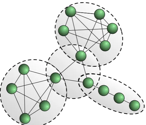
uptimealong with a periodicCPU-intensive probe program to calculate how much

CPU is available on a node. To minimise the intrusiveness of this probe, NWS reduces the frequency of the probes when recent availability measurements are approximately static, and increases them as availability changes.

The second set of sensor data is measurement of the end-to-end network per-formance between pairs of compute nodes using two active probes: one which measures the round-trip time of a small TCP message, and the other using a large message. From this, the bandwidth and latency of a link, along with the time to open a TCP socket can be inferred.

(44)

Each of these representative sensors measure inter-node performance with each other in turn, and this continues up the hierarchy until the root clique.

The Forecaster component uses the time-stamped data from the Persistent State servers to generate forecasts of the performance data on demand. These are com-puted using a set of forecasting models to predict the recent and current measure-ments based on historical data and comparing them with the actual measuremeasure-ments (a technique dubbed postcasting). The model with smallest mean squared error is chosen as the best available, and is chosen to predict future performance data [Wol03].

Since the network and compute availability are continually changing, the perfor-mance data produced may be a non-stationary series, and limiting the amount of history available to a model may improve the accuracy of the resource predictions. NWS uses models with varying window sizes as part of the resource prediction process, and again uses the model with the smallest mean squared error.

Note that the predictions produced by NWS differ from those of an application model in that they are predictions of future availability of compute and network resources, rather than the resourceconsumptioncharacteristics of applications. Both pieces of information are required: an application model cannot produce accurate estimates of an application’s runtime if it does not know the resources available for that application to use.

2.2.2 MDS

The Monitoring and Discovery Service (MDS) is a built-in component of Globus that provides a scalable resource information system for grid services. It has evolved along with Globus through four major versions, and is designed to address the needs of grid computing infrastructure including tools such as resource brokers, meta-schedulers, and fault detection systems. These needs fall into the two cate-gories ofmonitoringanddiscovery.

(45)

[image:45.595.182.424.132.339.2]

Fig. 2.1: NWS clique hierarchy

A data model and naming system based on that of the Lightweight Directory Access Protocol (LDAP) was chosen by the Globus Alliance for MDSversion 1. The data model consists of set of elements, each of which has a type called an object class which is defined in a class hierarchy. The object class defines a set of mandatory and optional attributes for each element and what kinds of values each attribute may contain. In the case ofMDS, each element represents a grid resource, such as a compute node, or some network infrastructure. An example can be seen inFig. 2.2. The naming system is also based onLDAP. Each element has a unique identifier called a Distinguished Name (DN) which can be thought of as similar to the absolute path to a file. Entries are organised in a Directory Information Tree (DIT) where each entry is a child to some other entry, and each component in a DN ‘path’ represents a single specific DIT entry. Fig. 2.3shows an example distinguished name.

TheMDScould be queried and updated usingLDAP-style queries. For example, the query(&(objectClass=GlobusHost)(o=University of Warwick)(c=UK)(totalMemory>256000000))would

find all compute nodes at Warwick with more than 256MB of memory.