publisher policies. Please scroll down to view the document itself. Please refer to the repository record for this item and our policy information available from the repository home page for further information.
To see the final version of this paper please visit the publisher’s website. Access to the published version may require a subscription.
Author(s): Luciana Juvenal and Mark P. Taylor
Article Title: Threshold Adjustment of Deviations from the Law of One Price
Year of publication: 2008
R
EGIME-S
WITCHINGM
ODELS INE
CONOMICS ANDF
INANCEThreshold Adjustment of Deviations from the
Law of One Price
Luciana Juvenal
∗Mark P. Taylor
†∗Federal Reserve Bank of St. Louis, [email protected]
†University of Warwick; Barclays Global Investors and Centre for Economic Policy Research,
Abstract
Using self-exciting threshold autoregressive models, we explore the validity of the law of one price (LOOP) for sixteen sectors in nine European countries. We find strong evidence of nonlin-ear mean reversion in deviations from the LOOP and highlight the importance of modelling the real exchange rate in a nonlinear fashion in an attempt to measure speeds of real exchange rate adjustment. Using the US dollar as a reference currency, the half-lives of sectoral real exchange rate shocks, calculated by Monte Carlo integration, imply much faster adjustment than the ‘con-sensus’ half-life estimates of three to five years. The results also imply that transaction costs vary significantly across sectors and countries.
∗We are grateful to an editor of this journal (Gary Koop) and to two anonymous referees for helpful
1
Introduction
Purchasing power parity (PPP) is one of the oldest and most fundamental concepts in economics. Under PPP, aggregate price levels should be the same across countries once expressed in a common currency. A key building block of PPP is the so called Law of one price (LOOP), which states that, at the individual goods level, the prices of homogeneous goods should be the same in spatially separated markets once expressed in a common currency.
An assumption underlying the LOOP is that there is frictionless interna-tional goods arbitrage. In practice, it is often observed that prices of similar goods fail to equalize between countries. This evidence contradicts the idea of arbitrage postulated in the LOOP and it is a sign that markets are not completely integrated. One reason why prices of homogeneous commodities may not be the same across di¤erent countries is the existence of transaction costs arising from transport costs, tari¤s and nontari¤ barriers. A number of theoretical studies suggest the importance of transaction costs in modelling deviations from the LOOP (e.g. Dumas, 1992; Sercu et al., 1995; O’Connell, 1998). These studies argue that, due to frictions in international trade, devia-tions from the LOOP may be characterized by nonlinear adjustment. In par-ticular, the persistence of deviations from the LOOP will depend on whether the sectoral exchange rate has crossed a threshold that may re‡ect transac-tions costs. Simply put, if the cost of arbitraging is x percent, then there will be no incentive to arbitrage until the deviation from the LOOP has exceeded x percent. In this framework, we can potentially identify two regimes: within the threshold band deviations from the LOOP are indeterminate or border-line nonstationary and outside the band they are mean reverting towards the band because of the e¤ects of arbitrage. The …rst regime occurs when devi-ations from the LOOP are smaller than transaction costs and consequently are not worth arbitraging. In this case the real exchange rate will not exhibit any tendency to move back to equilibrium and the LOOP does not hold. In the second regime, deviations from the LOOP are higher than the transaction costs, arbitrage is pro…table and the process becomes mean reverting.
presence of a ‘band of inaction’ within which no trade takes place. Hence, inside the band deviations from the LOOP exhibit unit root behavior. Outside the band the process can become mean reverting.
These empirical studies provide evidence of the presence of nonlinearities in deviations from the LOOP. However, they are sometimes criticized on three counts. The …rst is that they are based on relatively few commodities or currencies. The second is related to the temporal aggregation problem that arises when using annual or quarterly data, such that the degree of upward bias in the estimated persistence of the real exchange rate rises with the degree of temporal aggregation in the data (see e.g. Taylor, 2001).1 The third is
associated with calculation of the speed of mean reversion, which is usually considered to be given by the autoregressive process outside the band and ignores the adjustment process of the model as a whole.
In order to overcome the …rst two limitations, in our paper we use a highly disaggregated monthly database previously analyzed by Imbs et al. (2003, 2005). The main di¤erence between the work of Imbs et al. (2003) and our paper is that the former focuses on the determinants of international trade segmentation. In contrast, our goal is to examine the general validity of the LOOP. In order to do this, we show that the low power of standard unit root tests motivates the study of deviations from the LOOP in a nonlinear fashion. In particular, we test the validity of modelling deviations from the LOOP allowing for nonlinearities and estimate a TAR model for each sectoral real exchange rate.
More precisely, in our baseline speci…cation we investigate the presence of threshold-type nonlinearities in deviations from the LOOP using real dollar sectoral exchange rates vis-à-vis nine major European currencies for sixteen sectors over the period 1981-1998. A total of one hundred and 43 sectoral real
1In a related study, Paya and Peel (2006) generate arti…cial data at high frequency from
exchange rates are analyzed2. Nonlinearities are modelled using a self-exciting
threshold autoregressive (SETAR) model.
Our results suggest that the SETAR model characterizes well deviations from the LOOP for a broad range of currencies and disaggregated goods sec-tors. We also …nd reasonable estimates of transaction costs and convergence speeds which are in line with the theoretical literature on transaction costs in international goods arbitrage. Overall, there is wide variation in the results across countries and across sectors. This is partly due to the di¤erent nature of the sectors analyzed. In addition, there is also a country e¤ect: some countries exhibit relatively low thresholds for a given sector.
There is a certain consensus in the literature that aggregate real exchange rates may converge to a long-run equilibrium but that the speed at which this occurs seems to be very slow (Lothian and Taylor, 1996, 1997; Taylor, 1995, 2003; Rogo¤, 1996).3 A standard measure of the speed of mean reversion is
the half-life, which is the time taken for half of the e¤ects of a real exchange rate shock to die out. Rogo¤ (1996) points out that the ‘consensus estimates’ of the half-lives of shocks to the real exchange rate are typically in the range of three to …ve years. Since the short-run volatility in real exchange rates suggest that real exchange rate shocks typically arise mainly due to monetary or …nancial shocks, these shocks can have real e¤ects on the macroeconomy and on macroeconomic variables such as the real exchange only because of the presence of nominal rigidities. However, half-lives from three to …ve years seem much too large to be explained by nominal rigidities. Hence, Rogo¤ (1996) terms this result the ‘Purchasing Power Parity Puzzle’.4
The method of calculation of the half-life of adjustment turns out to be of the utmost importance to examine the PPP puzzle. Interestingly, previous
2Due to missing data we do not have one hundred and 44 exchange rate time series. 3This literature has tended to concentrate on necessary conditions for long-run absolute
purchasing power parity to hold. An exception is the recent paper by Coakley, Flood, Fuertes and Taylor (2005), who test for long-run relative PPP.
4Since Rogo¤’s (1996) paper, there has been a great deal of research e¤ort directed
studies of deviations from the LOOP using a SETAR model calculate the half-life based on the speed of convergence in the outer regime of the model. In other words, they compute the convergence relative to the threshold band as if it were a linear model. While some studies emphasized that it was not clear whether the method of computation of half-lives for linear models was applicable to nonlinear models (e.g. Lo and Zivot, 2001), it became a convention to use this measure. In order to shed some light on the mean-reverting properties of the sectoral real exchange rates we consider the regime switching that takes place within and outside the band in the SETAR model. In particular, we compute the half-lives using the procedure for estimating generalized impulse response functions described in Koop, Pesaran and Potter (1996), thus distinguishing the present paper from most of the previous empirical literature on this topic.5
Our results show that the speed of mean reversion depends on the size of the shocks. Larger shocks mean-revert much faster than smaller ones. In a minority of cases, our nonlinear model yields half-lives consistent with the ‘consensus’estimates of three to …ve years for small shocks. For larger shocks, however, all half-lives much smaller than three years are reported.
Overall, our results con…rm the importance of deviating from a linear spec-i…cation when modelling deviations from the LOOP (Taylor, Peel and Sarno, 2001; Sarno, Taylor and Chowdhury, 2004), shed some light to the problem of temporal aggregation analyzed in Taylor (2001) and also highlight the im-portance of calculating half-lives taking into account the SETAR model as a whole rather than just the outer regimes.
The remainder of the paper is organized as follows. Section 2 presents the motivation for modelling the exchange rate in a nonlinear fashion. Section 3 outlines the Self-Exciting Threshold Autoregressive (SETAR) model to be es-timated and the econometric techniques we employ. Section 4 presents results of tests for nonlinearity. Section 5 describes the data to be used. Prelimi-nary unit root tests results are discussed in Section 6 and Section 7 contains our estimation results and diagnostic tests. Finally, we make some concluding comments in Section 8.
5Taylor, Peel and Sarno (2001) also compute the half-lives using generalized impulse
2
Nonlinear Exchange Rate Dynamics:
Em-pirical Evidence and Theoretical Framework
The LOOP states that once prices are converted to a common currency, ho-mogenous goods should sell for the same price in di¤erent countries. Using the US as the reference country, let us de…ne deviations from the LOOP for countryi in sector j at timet as
qjti =sit+pijt pU Sjt (1)
where sit is the logarithm of the nominal exchange rate between country
i’s currency and the US dollar (de…ned as the number of dollars per unit of foreign currency)6, pi
jt is the logarithm of the price of good j in country i at
time t and pU S
jt is the logarithm of the price of good j in the U S at time t.
The idea behind the LOOP is that if prices of identical goods di¤er in two countries there is a pro…table arbitrage opportunity: the good can be bought in the country in which it costs less and sold at a higher price in the other country.
The failure of the LOOP has been documented in early studies (Isard, 1977; Richardson, 1978 and Giovannini, 1988). Within this strand of the literature, the evidence also suggests that deviations from the LOOP are signi…cant, very volatile and highly correlated with exchange rate movements.
The reasons why prices of similar goods may vary across locations has been widely analyzed in the international trade literature. One approach, which is the one we adopt in the present study, follows Heckscher’s (1916) idea that prices of homogeneous commodities may not be the same across di¤erent countries due to the existence of transaction costs in international arbitrage. If two homogeneous goods (once expressed in a common currency) are sold at di¤erent prices in two locations, the LOOP does not hold, and it will not be worth arbitraging and consequently lead to a price equalization unless the anticipated bene…t exceeds the transport costs between the two locations.
6As a consequence, an increase in the nominal exchange rate indicates an appreciation
These frictions to trade can imply the presence of nonlinearities in inter-national goods arbitrage. This idea began to be formalized in the theoretical literature in the 1980s and early 1990s (Williams and Wright, 1991; Dumas, 1992; Sercu et al., 1995). In these studies the lack of arbitrage arises from transaction costs such as transport costs. In most cases transport costs are modeled as a waste of resources— if a unit of good is shipped from one loca-tion to another, a fracloca-tion melts on its way, so that only a proporloca-tion of it arrives. These transaction costs create a ‘band of inaction’ for the real ex-change rate within which the marginal cost of arbitrage exceeds the marginal bene…t. Hence, within this band there is a no-trade zone and prices in two locations are disconnected.
It is clear that transport costs are not the only trade friction. In fact, the role of tari¤s and nontari¤ barriers as a potential driver of price di¤erentials between countries has also been explored. Tari¤s clearly create a wedge be-tween domestic and foreign prices. Although they have been falling in the last decades, they are still important for some commodities. Nontari¤ barri-ers may be another source of friction in international goods arbitrage but the empirical evidence o¤ers mixed …ndings on its relevance to explain deviations from the LOOP. Knetter (1994), for example, argues that nontari¤ barriers are important empirically to explain deviations from PPP. In contrast, Obstfeld and Taylor (1997) do not …nd nontari¤ barriers to be a signi…cant explanator of deviations from the LOOP.
Another factor that may lead to a failure of goods market arbitrage is the presence of nontraded components in goods that appear to be highly trad-able. This becomes more relevant when consumer price indices are considered. Labour costs and taxes, for example, are likely to di¤er across di¤erent loca-tions and they may a¤ect …nal local goods prices.
Overall, all of these frictions can create a wedge between prices of di¤erent countries and the estimated transaction costs band may be wider than the one implied by transport costs7. This point was considered in Dumas (1992). He studies a two-country general equilibrium model in the framework of a
ho-7As a reference point, an estimate of international transportation costs can be obtained
mogenous investment-consumption good. Dumas …nds that in the presence of sunk costs of arbitrage and random productivity shocks trade takes place only when there are su¢ ciently large arbitrage opportunities. When this happens the real exchange rate displays mean-reverting properties.
O’Conell and Wei (2002) extend the analysis using a broader interpretation of market frictions operating at the level of technology and preferences. Their model also allows for …xed and proportional market frictions. When both types of costs of trade are present they …nd that two ‘bands’ for deviations from the LOOP are generated. The idea is that arbitrage will be strong when it is pro…table enough to outweigh the initial …xed cost. In the presence of proportional arbitrage costs, the quantity of adjustments are very small, su¢ cient to prevent price deviations from growing but insu¢ cient to return the LOOP deviations to equilibrium.
Based on these theoretical studies, it is possible to estimate a model in which the real exchange rate has no tendency to adjust unless it has crossed a threshold equal to the transaction costs. This implies that within the threshold band changes in the real exchange rate are random and outside the band the process can become mean reverting when arbitrage takes place. This kind of model is the TAR (Tong, 1990) and it applies to individual commodities. Re-cent studies that analyze deviations from the LOOP in a threshold-type frame-work include Obstfeld and Taylor (1997), Taylor (2001), Imbs et al. (2003) and Sarno, Taylor and Chowdhury (2004).
Obstfeld and Taylor (1997) use aggregated and disaggregated data on cloth-ing, food and fuel for 32 city and country locations employing monthly data from 1980 to 1995. They estimate the half-lives of deviations from the LOOP as well as the thresholds. Their location average estimated thresholds are be-tween 7% and 10%. They also …nd a considerable variation in their estimates across sectors and countries.
Taylor (2001) investigates the impact of temporal aggregation in the data when testing for the LOOP. Using a Monte Carlo experiment with an arti-…cial nonlinear data generating process he …nds that the upward bias in the estimated half-lives rises with the degree of temporal aggregation. He also shows that the estimated half-lives have a considerable bias when the model is assumed to be linear when in fact there is a nonlinear adjustment.
real exchange rates. Although they do not directly report the results of their TAR estimation (because that is not the main point of their paper), they claim strong evidence of mean reversion.
Sarno, Taylor and Chowdhury (2004) use annual data on prices (interpo-lated into quarterly) for nine sectors and quarterly data on …ve exchange rates
vis-à-vis the US dollar (UK pound, French franc, German mark, Italian lira and Japanese yen) from 1974 to 1993. Using a SETAR model, they …nd strong evidence of nonlinear mean reversion with half-lives and threshold estimates varying considerably both across countries and across sectors.
In summary, all of these studies …nd supportive evidence of the LOOP when allowing for nonlinear exchange rate adjustment. Mean reversion takes place when LOOP deviations are large enough to allow for pro…table arbitrage opportunities.
All the previous studies use a TAR model to analyze the validity of the LOOP. As noted by Taylor, Peel and Sarno (2001) and Taylor and Taylor (2004), this model is very appealing in the context of individual goods but it is clear that for the aggregate real exchange rate it may be inappropriate. Transaction costs are likely to di¤er across sectors and consequently the speed of arbitrage may di¤er across goods. One could think that the aggregate real exchange rate is made up of goods prices with di¤erent implied thresholds. Some of these thresholds may be small and others will be larger. This means that as the real exchange rate moves away from equilibrium, more thresholds are crossed and thus the arbitrage forces become more powerful. Hence, one could expect that adjustment of the aggregate real exchange rate would be smooth rather than discrete and that the speed of adjustment would increase with the size of the deviation from equilibrium.8
The approach from the present paper di¤ers from previous studies for at least three reasons. First, in contrast to studies that use data at the quarterly frequency, we intend to overcome the temporal aggregation bias described in Taylor (2001) using a highly disaggregated monthly database. Second, we estimate a SETAR model without imposing the lag length. In particular, we choose the optimal lag on the basis of an information criterion. Finally, we compute the half-lives of deviations from the LOOP using generalized impulse
8This can be modeled using a smooth transition autoregressive (STAR) speci…cation.
response functions.
3
Econometric Method: Model and
Estima-tion
The theoretical models described in the previous section motivate the study of deviations from the LOOP using a nonlinear model. As explained before, the presence of transaction costs may generate a ‘band of inaction’(or thresholds) within which the costs of arbitrage exceed its bene…ts. Hence, inside the band, there is a no-trade zone where deviations from the LOOP are persistent. Once above or below this band, arbitrage takes place and deviations from the LOOP could become mean reverting.9 Empirically, this pattern is described by a threshold autoregressive (TAR) model, which was originally popularized by Balke and Fomby (1997) in the context of testing for PPP and the LOOP.
Denote the real exchange rate (deviations from the LOOP) for a sector j
in country i at time t as qi
jt. A simple three-regime TAR model (TAR) may
be written as
qijt = qjti 1+
PP1
p=1
p qjt pi +" i
jt if q i
jt d 6 (2)
qijt = ( 1 1) (qjti 1 ) +
P
P
p=2 p
(qijt p ) +"ijt if qjt di > (3)
qijt = ( 1 1) (qjti 1+ ) +
P
P
p=2 p
(qjt pi + ) +"ijt if qijt d< (4)
i
jt N(0; 2) (5)
9The discrete switching implied by the TAR model seems appealing when considering
where is the di¤erence operator, is the threshold parameter, qi jt d
is the threshold variable for sector i and country j, p is the autoregressive order selected via the Akaike Criterion and d denotes the delay parameter— an integer chosen from the set 2 1; d : The delay parameter captures the idea that it takes time for economic agents to react to deviations from the LOOP. The error term is assumed to be independently and identically distributed (iid) Gaussian.
This type of model in which the threshold variable is assumed to be the lagged dependent variable is called Self-Exciting TAR (SETAR). Hence, the model outlined is a SETAR (p;2; d), where 2 refers to the fact that there are two thresholds. Following Obstfeld and Taylor (1997) we assume that the thresholds are symmetric (transaction costs are equal if prices are higher in one location or in another) and that arbitrage forces operate in the same way if deviations from the LOOP occur above or below the threshold band.
In order to account for the fact that deviations from the LOOP would be persistent within the threshold band, restrictions on the parameters can be adopted. In this case, we make the simplifying assumption that = 0: This implies that within the band, qi
jt d 6 , deviations from the LOOP follow a
unit root process. Given that arbitrage is not pro…table, in the inner regime
qi
jt shows no tendency to move back towards equilibrium.
In contrast, in the outer regime, qi
jt d > , deviations from the LOOP
switch to a di¤erent autoregressive process that is stationary and hence has a tendency to revert to equilibrium if
P
P
p=1 p
<1. Note that this speci…cation assumes that reversion is towards the edge of the band.
We can rewrite the model in (2)-(5) together with the restriction = 0
using the indicator functions1 qjt di > ,1 qijt d< and 1 qjt di 6 , each of which takes value equal to one if the inequality is satis…ed and zero otherwise
qjti = ( 1 1) (qjti 1 ) +
P
P
p=2 p
(qjt pi ) 1 qijt d> +
PP1
p=1
p qjt pi 1 q i
jt d 6 + (6)
( 1 1) (qjti 1+ ) +
P
P
p=2 p
For purposes of exposition, re-write equation (6) as
qijt =Bjti ( ; d)0 + ijt (7) where Bi
jt( ; d)0 is a (1 3) row vector that describes the behavior of
qjti in the outer and inner regimes and is a (3 1) vector containing the autoregressive parameters to be estimated. In particular,
Bjti ( ; d)0 = X01 qi
jt d > Y
0
1 qi
jt d 6 Z01 qjt di < (8)
where,
X0 = (qi
jt 1 ) (qjti 2 ) ::: (qjt pi ) ,
Y0 = qi
jt 1 qjti 2 ::: qjt pi and
Z0 = (qi
jt 1+ ) (qijt 2+ ) ::: (qijt p+ ) :
Also,
0 =
where,
0 =
1 1 2 3 ::: p and 0 = 1 2 ::: p 1 0 :
The parameters of interest are , and d. Equation (8) is a regression equation nonlinear in parameters and can be consistently estimated under weak regularity conditions using nonlinear using least squares. For a given value of and d the least squares estimate of is
b( ; d) =
T
X
t=1
Bijt( ; d)Bjti ( ; d)0
! 1 T
X
t=1
Bijt( ; d) qjti
!
(9)
with residualsbijt( ; d) = qi
jt Bjti ( ; d)0b( ; d), and residual variance
b2( ; d) = 1
T
T
X
t=1
bijt( ; d)
2 (10)
identify the model in (7) that consists on the simultaneous estimation of , and d via a grid search. The model is estimated by sequential least squares for integer values of d from 1 to d p. The values of and d that minimize the sum of squared residuals are chosen. This can be written as
b;db = arg min
2 ; d2 b
2
( ; d) (11)
where = [ ; ]:
The least squares estimator of isb =b b;db with residualsbi
jt b;db =
qi
jt Bjti (b;db)0b b;db and residual variance b
2
b;db = T1
T
X
t=1
bijt b;db
2
.
4
Testing for Nonlinearity
Before analyzing the results from the estimation of the SETAR model, it is important to test whether the nonlinear speci…cation is superior to a linear model.
As noted by Hansen (1997), testing this hypothesis is not that straightfor-ward. A statistical problem is present because conventional test statistics to test the null hypothesis of a linear autoregressive model against the alterna-tive of a SETAR model have nonstandard asymptotic distributions due to the presence of nuisance parameters. These parameters are not identi…ed under the null hypothesis of linearity. It can be seen that in the model in (6) the nuisance parameters are the threshold and the delayd.
In order to overcome the inference problems derived from the nonstandard asymptotic distributions of the tests, Hansen (1997) developed a bootstrap method to replicate the asymptotic distribution of the classicF-statistic. This method requires the estimation of both the linear model under the null hy-pothesis and the TAR model under the alternative hyhy-pothesis.
If errors areiidthe null hypothesis of a linear model against the alternative can be tested using the statistic
FT( ; d) =T e
2
b2( ; d)
b2( ; d) ; (12)
where FT is the pointwise F-statistic when and d are known, T is the
corresponding to the linear AR(p) and SETAR (p;2; d) models, respectively. Since and d are not identi…ed under the null hypothesis, the distribu-tion of FT( ; d) is not central 2. Hansen (1997) shows that the asymptotic
distribution of FT( ; d) may be approximated using the following bootstrap
procedure. Letyijt; t= 1; :::; T beiid N(0;1)random draws, and set qijt =yjti . Using the observationsqi
jt 1; qjti 2; :::; qjt pi for t= 1; :::; T, regressyjti onqijt 1;
qi
jt 2; :::; qjt pi and estimate the restricted and unrestricted models and obtain
the residual variancese 2 andb 2( ; d), respectively. With these residual vari-ances, it is possible to calculate the following F-statistic:
FT( ; d) = T e
2
b 2( ; d)
b 2( ; d) : (13)
The bootstrap approximation to the asymptoticp-value of the test is calcu-lated by counting the number of bootstrap samples for whichFT( ; d)exceeds the observed FT( ; d).
5
Data
Data on disaggregated price levels for European countries was obtained from Eurostat10 and for the US was obtained from Eurostat and the US Bureau of Labour Statistics. The data set contains monthly observations on two-digit consumer prices (CPI) for sixteen goods categories. The period analyzed is 1981:01 to 1998:12. Our sample period ends in 1998 due to the introduction of the euro in January 1999. The countries covered are Belgium, Denmark, Germany, France, Italy, Netherlands, Portugal, Spain, UK and the US as a reference country. The sectors analyzed are: bread and cereals (bread), meat (meat), dairy products (dairy), fruits (fruits), tobacco (tobac), alcoholic and non alcoholic drinks (alco), clothing (cloth), footwear (foot), fuels and energy (fuel), furniture (furniture), domestic appliances (dom), vehicles (vehicles), communication (comm), sound and photographic equipment (sound), books (books) and hotels (hotels).
The monthly series on nominal dollar exchange rates are taken from the In-ternational Financial Statistics database of the International Monetary Fund.
Dollar sectoral real exchange rates qi
jt in logarithmic form are calculated
vis-à-vis the nine European currencies of the countries mentioned before in
the way de…ned in equation (1). Each series is demeaned in order to account for the existence of di¤erent long run equilibrium levels of the sectoral real exchange rate.
6
Unit Root Tests
The existence of a unit root in the sectoral real exchange rate is economically meaningful because it conveys that it has no tendency to adjust to its long-run equilibrium. Consequently, prices in di¤erent locations would have no tendency to equalize and the LOOP would not hold.
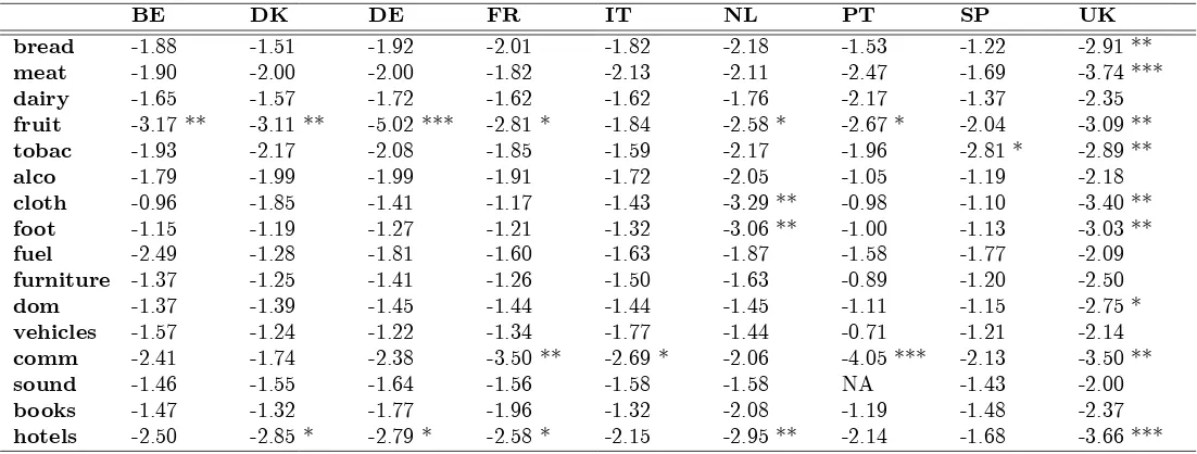
We tested the hypothesis that deviations from the LOOP are nonstationary by applying a battery of standard linear unit root tests. Table 1.A presents the Dickey-Fuller test (the other tests are not reported here but available from the authors upon request): for each of the sectoral exchange rates the null hypothesis of a unit root was generally not rejected at conventional signi…cance levels.
Given the high persistence of the real exchange rate, unit root tests tend to do a poor job in most cases. Table 2 shows a simulation of the power of the Dickey Fuller test forp=0.01 andp=0.05 signi…cance levels. The power of the test represents the number of times the test rejects the unit root null hypothesis given that the process is stationary. From these results it follows that the test does not perform well for highly persistent autoregressive processes (i.e. higher than 0.90). Given that the power is generally very low, the test is weak. This highlights the importance of accounting for nonlinearities when modelling real exchange rate dynamics. A failure to do this may lead us to conclude that the exchange rate follows a nonstationary process when in fact may be nonlinearly mean reverting.
Taylor (2001) points out that the problem of low power of conventional unit root tests is exacerbated when the true process is nonlinear. Assuming the real exchange rate follows an AR(1)process, he shows that when the exchange rate displays nonlinear adjustment, the estimate of the autoregressive parameter would be biased upwards (i.e. towards 1). This will bias the ‘t-statistic’ of the Dickey-Fuller test downwards in absolute value, making it more di¢ cult to reject the unit root null hypothesis.
In contrast to Taylor (2001), the shifts are modelled as a Markov chain. The study shows that when the data generating mechanism is stationary but the transition probabilities in the Markov process are highly persistent (as is the case for …nancial data) the unit root tests are very weak.
By and large, the general problem with standard unit root tests is that they assume a symmetric adjustment process. It is clear that if the true model is nonlinear, adjustment would be asymmetric. In order to account for this we applied the Enders and Granger (1998) threshold unit root test.11
The procedure developed by Enders and Granger (1998) can be understood as a generalization of the Dickey-Fuller test and can be used to test the null hypothesis of a unit root against an alternative of stationarity with threshold adjustment. Its main advantage is that in a wide range of cases it is more powerful than the Dickey-Fuller test. The test performs particularly better the more asymmetric is the process.
Table 1.B shows the results of the Enders and Granger test applied to our data. This test rejects the unit root null at the 5% level in around 30% of the series in contrast to a 15% rejection when employing the linear Dickey-Fuller test. A simulation of the power of the Enders and Granger test is presented in Table 2 for di¤erent values of the autoregressive parameter and =0.1. The test performs slightly better than the Dickey-Fuller test but the power nevertheless remains low for highly persistent series.
This analysis reinforces the argument of Taylor (2001) that it seems rea-sonable to replace the unit root null hypothesis with a stationary null when testing the validity of the LOOP given that the deviations from the LOOP may be stationary but have a local unit root in the inner regime.
7
Empirical Results
7.1
Estimation and linearity tests
In this section we explore the presence of a threshold-type nonlinearity in deviations from the LOOP. The test against a SETAR model requires the input of the parameters in the linear and nonlinear model. Hence, in this section we brie‡y describe the estimation process and the linearity test results.
11The authors are grateful to an anonymous referee for suggesting the discussion of this
We start by specifying a linear AR(p) model for each series of sectoral real exchange rates and choose the lag length according the Akaike criterion.12
We assume that this gives us the appropriate lag order for each regime of the SETAR model. Following Hansen (1997), the range for the grid search is selected to contain the 15th and 85th percentile of the threshold variable. This ensures that the model is well identi…ed for all thresholds and also that the results are not driven by a few outliers.13 The SETAR model is estimated
via a grid search over and d. As described above in Section 4, and d are selected through the minimization of the sum of squared residuals.
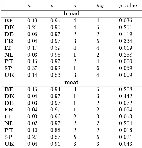
We next evaluate the adequacy of the estimated SETAR model using a battery of diagnostic tests on the estimated residuals. In particular, we start by examining the presence of serial correlation in the residuals using the Ljung-Box test. When serial correlation is found, we modify the model by increasing the value of the lag length (p). Then, we test for homoskedasticity of the residuals using the ARCH LM test. Neglected heteroskedasticity is potentially important in this context since it may lead to spurious rejection of the null hypothesis of linearity (see Franses and Van Dijk, 2000). We also evaluate the normality assumption using the Jarque-Bera test. The rejection of normality may indicate that there are outliers, that the residuals are heteroskedastic or that there is some other source of misspeci…cation. A …nal step involves examining whether the proposed model captures all the nonlinear features of the series. This can be analyzed by testing for remaining nonlinearity. In order to test for the presence of an additional regime in a SETAR model one needs to estimate the alternative multiple-regime model and evaluate it against the original SETAR model in a similar fashion as the nonlinear model is tested against a linear one. The estimation and evaluation of di¤erent multiple-regime SETAR models for 143 series can be very time consuming. Thus, we test for remaining nonlinearity using the Ramsey (1969) RESET test. This test leaves the type of nonlinearity under the alternative hypothesis unspeci…ed but it is useful for our purposes to evaluate the potential presence of misspeci…cation in our model. After running the diagnostic tests we make changes to our model
12We prefer the Akaike information criterion over the Schwartz information criterion
be-cause the former leads to well behaved residuals both in the linear and the nonlinear models.
13After estimating the SETAR model for each of the sectoral real exchange rates, we
when necessary.
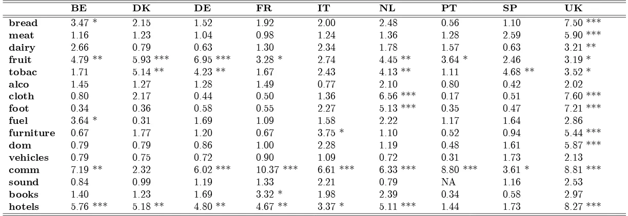
The estimated SETAR model for each sectoral real exchange rate is pre-sented in Table 3.A and Table 3.B shows the diagnostic tests. By and large, the estimated SETAR models pass the diagnostic tests. A relevant point to highlight is the violation of the normality assumption in the tobacco and communication sectors and, to a lesser extent, in the fuel sector. Thus, the estimated SETAR models for these sectors might be misspeci…ed.
Using the parameters from the SETAR and linear models, the bootstrapped
p-values for the Hansen test are calculated based on 1000 replications (see Hansen, 1997). The results from the linearity test, reported in Table 3.A, show that the null hypothesis of linearity is rejected in 104 out of 143 cases at a 10% level. At a 5% level the null hypothesis of linearity is rejected in 77 cases.
of taxation or sale regulations. Interestingly, we …nd evidence of nonlineari-ties in this sector. A possible explanation for this result is that the estimated SETAR model is misspeci…ed; for this sector there is a strong violation of the normality assumption.
7.2
SETAR model
Table 3.A reports the results for the SETAR model. From this table, it is clear that there is a wide variation in the results across countries and across sectors. Part of this is explained by the di¤erent nature of the sectors analyzed. Some sectors that involve high shipping costs and that are less homogeneous are clearly characterized by higher threshold bands. In addition, a country e¤ect seems to be present. For a given sector, some countries exhibit relatively lower thresholds.
In discussing our results further in this Section, greater emphasis will be given to the behavior of tradable sectors or to sectors which at …rst glance appear to be tradable and we will focus mainly on those cases in which non-linearities are signi…cant.
7.2.1 Transaction costs
Estimated transaction costs di¤er enormously across sectors and countries. Relatively high transaction costs are observed for furniture, sound and vehicles, with average thresholds being 24%, 20% and 19%, respectively. Within these sectors, there is certain heterogeneity in the value of transaction costs across countries. Considering the countries for which nonlinearities are detected, the estimated b ranges from 10% to 35% for furniture, from 10% to 29% for sound and from 4% to 30% for vehicles. It seems reasonable to …nd high threshold bands for these sectors given their high shipping costs and their high degree of di¤erentiation. The domestic appliances sector exhibits an average threshold band of 17%, ranging from 6% in Germany to 32% in Spain. The high transaction costs of this sector could be due to the barriers to arbitrage caused by di¤erences in international regulatory standards.
(19%). In the footwear sector, evidence of nonlinearities are found for all countries except Spain and the UK. The highest transaction costs correspond to Denmark (33%) and the lowest to the Netherlands (5%).
As far as the international fruit market is concerned, Denmark and the US appear to be highly integrated given that b is 2%. Other countries, such as Germany, Spain and the UK seem to be less integrated with estimated threshold of 11%, 12% and 15%, respectively.
Overall, the estimation results suggest that in some cases the value of the transaction costs is sector speci…c. This result is the most common …nd-ing mentioned in the literature (see Imbs et al., 2003). The sector e¤ect is observed, for example, in the case of furniture, sound and vehicles, where thresholds are relatively high.
A result less mentioned in the literature is the country e¤ect. By and large, there are ‘low-threshold countries’such as Denmark, France, Germany, Netherlands and the UK and ‘high-threshold countries’such as Belgium, Italy, Spain and Portugal. Average estimated transaction costs estimates for the for-mer group range from 10% (UK and France) to 14% (Denmark and Germany). For the latter group, average threshold estimates range from 16% (Belgium) to 21% (Italy)14.
In comparison to the work of Obstfeld and Taylor (1997) our estimated threshold bands are slightly higher, ranging from 10% to 21% (country aver-ages), compared to the range reported by Obstfeld and Taylor of 7% to 10%. However, considering only European countries, the Obstfeld-Taylor range be-comes 9% to 19%, which is closer to our estimated range. In addition, Obstfeld and Taylor (1997) use a much less disaggregated database and this could create another source of di¤erence with respect to our estimated thresholds.
In line with the results described in Imbs et al. (2003), we …nd that the estimated thresholds are higher for goods with larger estimated persistence using a linear AR(p) model.
7.2.2 Half-lives
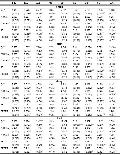
A standard measure of the speed of mean reversion is the half-life, which is the time it takes for half of the initial e¤ect of a shock to dissipate. Table
14Speci…cally, average estimated transaction costs are 10% for the UK and France, 11%
4.A reports the estimated half-lives of deviations from the LOOP using two di¤erent methodologies. First, we compute the speed of mean reversion for each sectoral real exchange rate in the outer regime. Given that in the SETAR model the real exchange rate is at equilibrium within the band [ ; ], it is reasonable to focus …rst on convergence to equilibrium relative to the band. In this case, the speed of convergence is given by the outer root of the TAR process, de…ned as =
P
P
p=1 p
. The half-life is calculated as in a linear model, i.e. hl=ln0.5/ln : Some studies emphasize that it is not clear whether the computation of half-lives for linear models is applicable for nonlinear models (see Lo and Zivot, 2001). However, all the studies based on a SETAR model use this measure (see, for example, Taylor, 2001) and thus we report it here for a simple comparison.
While the estimated half-lives of the outer regime give some insights about the speed of mean reversion, this measure has the limitation that it does not consider the regime switching that takes place within and outside the band. Thus, in order to shed some light on the mean reverting properties of the sec-toral real exchange rates we also calculate the half-lives using the generalized impulse response functions procedure described in Koop, Pesaran and Potter (1996). This complementary calculation, which considers the SETAR model as a whole, is important in the context of our model because there is an in…-nite half-life within the band and a half-life depending on outside the band. A shock may cause the model to switch regimes and this adjustment is not captured using the …rst methodology. These results can be compared to those obtained using the …rst methodology and also to those previously reported in the literature to see if modeling nonlinearities helps to resolve the PPP puzzle of very slow real exchange rate adjustment (Rogo¤, 1996).
One issue that arises in the context of nonlinear models is that the shape of impulse responses depends on the history of the system at the time of the shock, the size of the shock and the distribution of future exogenous inno-vations. Following Taylor et al. (2001), we compute the impulse response functions conditional on average initial history using Monte Carlo integra-tion.15
15For a complete explanation of generalized impulse responses see Koop et al. (1996).
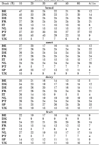
For each sectoral real exchange rate, we estimate impulse responses condi-tional on average initial history for shocks of 10%, 20%, 30%, 40%, 50% and 60% and compute the half-lives for each shock size. This allows us to compare the persistence of large and small shock sizes. Table 4.A reports the half-lives for each shock as well as the half-lives implied by the conventional estimation procedure. Tables 4.B and 4.C show the average half-lives at a country and sectoral level.
From these tables it is clear that the speed of mean reversion depends on the size of the shock. Larger shocks mean-revert much faster than smaller shocks. This happens because the half-lives are dependent on the root of the outer regime as well as on the size of the threshold. Mean reversion is slower the closer the exchange rate is to equilibrium, given by the threshold bands. In addition, these results highlight the importance of calculating the half-lives using generalized impulse response functions. The conventional method gives a much faster speed of mean reversion. However, the latter result should be interpreted carefully, given that the conventional method considers only the outer regime and does not account for the regime shifts of the SETAR model. Using country averages, half-lives are between 19 to 43 months for a 10% shock and between 10 to 25 months for a 60% shock. By contrast the half-lives computed using the conventional methodology range from 7 to 22 months.
The UK shows fast mean reversion, ranging from an average half-life of 19 months for a shock of 10% to one year for shocks of 60%; for shocks of 20% to 40%, the half-lives are between 14 and 12 months. The UK average half-life implied by the outer regime is 9 months. France exhibits considerably higher persistence, with average half-lives ranging from 33 months for a 10% shock to 25 months for 50% and 60% shocks. The average half-lives of Germany are very close to those of France, ranging from 34 months for a 10% shock to 20 months for a 60% shock.
These results shed some light on the PPP puzzle (Rogo¤, 1996). In par-ticular, our nonlinear models yield half-lives consistent with the ‘consensus’ estimates of 3 to 5 years only for small shocks taking place when the real ex-change rate is close to equilibrium. For Germany, France, Italy, Netherlands and the UK, even small shocks of 10% have a half-life of under 3 years. For shocks larger than 20% all of the countries exhibit a half-life under 3 years.
Our results also show that the half-life of deviations are considerably
duced when …tting a nonlinear model with respect to a linear AR(p) model. By and large, a linear model yields estimated speeds of adjustment consistent with the PPP puzzle. The half-lives implied by the linear model are between 20 and 230 months (country averages).16
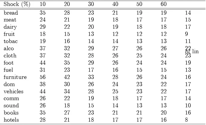
The half-lives at the country level display heterogeneity across sectors. From Table 4.C it is clear that the pattern of larger shocks adjusting faster is also very marked at the sectoral level, however. Relatively high persistence is observed in furniture and vehicles (for all shock sizes), followed by alcoholic and nonalcoholic beverages, clothing and footwear. The sectors with the lowest persistence for all shocks sizes are fruits, tobacco, sound and fuel.
It is di¢ cult to compare these results with those reported in the related literature given that studies using SETAR models for disaggregated data com-pute the half-lives in the outer regime. Obstfeld and Taylor (1997), for exam-ple, estimate half-lives ranging from 3 to 19 months. These results are in line with those reported here for the conventional (outer-regime) calculation. In-terestingly, our estimated half-lives for larger shocks are relatively lower than the ones reported in studies where data at lower frequency was used (Sarno, Taylor and Chowdhury, 2002, for example, …nd an average estimated half-life of 6 quarters). These results underline the relevance of modelling deviations from the LOOP in a nonlinear framework using data at higher frequency and the importance of calculating half-lives taking into account the SETAR model as a whole using generalized impulse response functions.
7.2.3 The delay parameter
The estimation results for the SETAR model suggest that the speed at which agents react to deviations from the LOOP is heterogeneous across sectors and across countries for a given sector. In principle, one should not expect that deviations from the LOOP to exhibit a high degree of stickiness (large values of d). In fact, in 48 out of the 143 cases examined, our estimation results report a delay parameter equal to 1 and most of the estimated values ofd are equal to 2 or 3. Overall, the modal estimate of the delay parameter is 3.
Given that the estimated delay parameter di¤ers from 1 in a majority of cases, it seems reasonable to estimate it within the grid search. Obstfeld and
16The results of the linear model estmation are not presented here, in order to conserve
Taylor (1997) restrict it to equal 1. However, we should not expect the results to vary considerably with di¤erent values of the delay parameter.
As a robustness check, the model was estimated restrictingdto equal unity (results not presented here but available from the authors upon request). It turns out that the estimated parameters do not change considerably from one speci…cation to the other. The sum of squared residuals also remains very stable in the di¤erent speci…cations. This is a desirable result because it means that the estimated parameters are not determined by accidental features of the data.
8
Conclusion
In this study we …nd that when modelling deviations from the LOOP in a nonlinear fashion we …nd evidence supportive of mean reversion in sectoral real exchange rates. There is, however, evidence of considerable heterogeneity in transaction costs across both sectors and countries. Using the US dollar as the reference currency, the estimated threshold bands range from 10% to 21% (measured as country averages).
frequency.
The time taken for economic agents to react to deviations from the LOOP varies across sectors and countries. The modal value of the delay parameter is 3. This may suggest that the delay parameter should be estimated and not restricted to be equal to unity as has been done in previous studies, although our results are robust and the estimated parameters do not change considerably when d is restricted to equal unity.
A
Appendix: Tables
Table 1.A. Dickey-Fuller Test
BE DK DE FR IT NL PT SP UK
bread -1.88 -1.51 -1.92 -2.01 -1.82 -2.18 -1.53 -1.22 -2.91 **
meat -1.90 -2.00 -2.00 -1.82 -2.13 -2.11 -2.47 -1.69 -3.74 ***
dairy -1.65 -1.57 -1.72 -1.62 -1.62 -1.76 -2.17 -1.37 -2.35
fruit -3.17 ** -3.11 ** -5.02 *** -2.81 * -1.84 -2.58 * -2.67 * -2.04 -3.09 **
tobac -1.93 -2.17 -2.08 -1.85 -1.59 -2.17 -1.96 -2.81 * -2.89 **
alco -1.79 -1.99 -1.99 -1.91 -1.72 -2.05 -1.05 -1.19 -2.18
cloth -0.96 -1.85 -1.41 -1.17 -1.43 -3.29 ** -0.98 -1.10 -3.40 **
foot -1.15 -1.19 -1.27 -1.21 -1.32 -3.06 ** -1.00 -1.13 -3.03 **
fuel -2.49 -1.28 -1.81 -1.60 -1.63 -1.87 -1.58 -1.77 -2.09
furniture -1.37 -1.25 -1.41 -1.26 -1.50 -1.63 -0.89 -1.20 -2.50
dom -1.37 -1.39 -1.45 -1.44 -1.44 -1.45 -1.11 -1.15 -2.75 *
vehicles -1.57 -1.24 -1.22 -1.34 -1.77 -1.44 -0.71 -1.21 -2.14
comm -2.41 -1.74 -2.38 -3.50 ** -2.69 * -2.06 -4.05 *** -2.13 -3.50 **
sound -1.46 -1.55 -1.64 -1.56 -1.58 -1.58 NA -1.43 -2.00
books -1.47 -1.32 -1.77 -1.96 -1.32 -2.08 -1.19 -1.48 -2.37
hotels -2.50 -2.85 * -2.79 * -2.58 * -2.15 -2.95 ** -2.14 -1.68 -3.66 ***
Table 1.B. Enders and Granger Test
BE DK DE FR IT NL PT SP UK
bread 3.47 * 2.15 1.52 1.92 2.00 2.48 0.56 1.10 7.50 ***
meat 1.16 1.23 1.04 0.98 1.24 1.36 1.28 2.59 5.90 ***
dairy 2.66 0.79 0.63 1.30 2.34 1.78 1.57 0.63 3.21 **
fruit 4.79 ** 5.93 *** 6.95 *** 3.28 * 2.74 4.45 ** 3.64 * 2.46 3.19 *
tobac 1.71 5.14 ** 4.23 ** 1.67 2.43 4.13 ** 1.11 4.68 ** 3.52 *
alco 1.45 1.27 1.28 1.49 0.77 2.10 0.80 0.42 2.02
cloth 0.80 2.17 0.44 0.50 1.36 6.56 *** 0.17 0.51 7.60 ***
foot 0.34 0.36 0.58 0.55 2.27 5.13 *** 0.35 0.47 7.21 ***
fuel 3.64 * 0.31 1.69 1.09 1.58 2.22 1.17 1.64 2.86
furniture 0.67 1.77 1.20 0.67 3.75 * 1.10 0.52 0.94 5.44 ***
dom 0.79 0.79 0.86 1.00 2.28 1.19 0.48 1.61 5.87 ***
vehicles 0.79 0.75 0.72 0.90 1.09 0.72 0.31 1.73 2.13
comm 7.19 ** 2.32 6.02 *** 10.37 *** 6.61 *** 6.33 *** 8.80 *** 3.61 * 8.81 ***
sound 0.84 0.99 1.19 1.33 2.21 0.79 NA 1.16 2.53
books 1.40 1.23 1.69 3.32 * 1.98 2.39 0.34 0.58 2.97
hotels 5.76 *** 5.18 ** 4.80 ** 4.67 ** 3.37 * 5.11 *** 1.44 1.73 8.27 ***
Table 2. Power of the Unit Root Test (1% and 5% signi…cance levels)
Dickey-Fuller Test Enders and Granger Test
p=0.01 p=0.05 p=0.01 p=0.05 =0.80 51.89 87.9 57.34 91.2 =0.90 9.06 32.33 15.19 36.18 =0.95 2.78 12.38 7.96 17.43 =0.96 1.93 9.94 5.64 13.27 =0.97 1.44 8.14 4.92 12.41 =0.98 1.4 6.83 4.87 11.74
Notes: The table shows the power of the Dickey Fuller and the Enders and Granger tests at 1% and 5%signi…cance levels. The results were caluclated on the basis of 10,000 replications and T=200. In the case of the Dickey-Fuller test, we assumed that the true process follows an AR(1) model with autoregressive pa-rameter . In the case of the Enders and Granger test we assumed that the process follows a SETAR (1,2,1) model similar to that in equation 6 with =0.10 and outer root .
Table 3.A. SETAR estimation results
d lag p-value
bread
BE 0.19 0.95 4 4 0.036
DK 0.21 0.95 4 5 0.251
DE 0.05 0.97 2 2 0.119
FR 0.04 0.97 3 5 0.334
IT 0.17 0.89 4 4 0.019
NL 0.03 0.96 1 2 0.258
PT 0.15 0.97 2 4 0.000
SP 0.37 0.92 1 6 0.059
UK 0.14 0.83 3 4 0.009
meat
BE 0.15 0.94 3 5 0.208
DK 0.04 0.97 1 3 0.442
DE 0.03 0.97 1 2 0.072
FR 0.04 0.97 1 2 0.094
IT 0.03 0.96 2 3 0.053
NL 0.02 0.97 2 2 0.204
PT 0.10 0.88 2 2 0.018
SP 0.27 0.87 5 5 0.021
UK 0.04 0.91 3 3 0.043
[image:30.612.174.423.365.624.2]dairy
BE 0.22 0.91 4 4 0.011
DK 0.20 0.94 1 5 0.077
DE 0.20 0.94 1 3 0.128
FR 0.05 0.97 1 4 0.072
IT 0.22 0.86 3 4 0.038
NL 0.07 0.96 3 3 0.042
PT 0.03 0.97 2 2 0.016
SP 0.10 0.98 1 3 0.016
UK 0.03 0.96 2 4 0.027
fruit
BE 0.16 0.93 6 8 0.044
DK 0.02 0.92 2 2 0.009
DE 0.11 0.95 10 12 0.076
FR 0.18 0.91 3 8 0.023
IT 0.22 0.83 1 2 0.024
NL 0.14 0.95 1 8 0.688
PT 0.18 0.84 8 9 0.044
SP 0.12 0.93 1 1 0.046
UK 0.15 0.92 1 12 0.069
tobac
BE 0.03 0.97 3 11 0.203
DK 0.03 0.97 1 4 0.022
DE 0.19 0.78 1 3 0.097
FR 0.08 0.97 2 2 0.054
IT 0.20 0.76 1 2 0.003
NL 0.12 0.90 2 4 0.024
PT 0.29 0.82 2 2 0.010
SP 0.05 0.95 1 2 0.097
UK 0.15 0.89 1 2 0.049
alco
BE 0.05 0.97 1 2 0.094
DK 0.09 0.94 1 4 0.018
DE 0.17 0.95 4 4 0.029
FR 0.02 0.97 1 4 0.072
IT 0.07 0.97 2 4 0.032
NL 0.04 0.97 1 2 0.173
PT 0.30 0.98 2 2 0.010
SP 0.11 0.98 1 5 0.128
UK 0.08 0.94 4 4 0.060
...table 3.A. continued
d lag p-value
cloth
BE 0.25 0.97 4 5 0.068
DK 0.09 0.97 2 8 0.086
DE 0.19 0.96 4 4 0.061
FR 0.08 0.98 1 4 0.034
IT 0.32 0.92 2 4 0.006
NL 0.03 0.93 4 8 0.853
PT 0.14 0.98 2 3 0.017
SP 0.08 0.98 1 5 0.224
UK 0.02 0.93 3 7 0.296
foot
BE 0.27 0.96 3 5 0.079
DK 0.33 0.89 5 7 0.022
DE 0.22 0.96 4 4 0.052
FR 0.07 0.98 5 5 0.063
IT 0.27 0.95 5 5 0.008
NL 0.05 0.92 4 9 0.002
PT 0.12 0.98 3 3 0.038
SP 0.07 0.98 1 6 0.124
UK 0.15 0.90 2 3 0.119
continued next page... ...table 3.A. continued
d lag p-value
fuel
BE 0.04 0.95 2 5 0.206
DK 0.29 0.84 9 10 0.000
DE 0.04 0.97 2 2 0.122
FR 0.05 0.97 2 4 0.098
IT 0.25 0.88 2 2 0.016
NL 0.06 0.96 1 2 0.220
PT 0.23 0.87 1 2 0.004
SP 0.21 0.84 2 2 0.009
UK 0.08 0.95 1 4 0.019
furniture
BE 0.27 0.96 4 4 0.090
DK 0.24 0.97 2 3 0.047
DE 0.18 0.96 1 2 0.056
FR 0.10 0.98 2 4 0.028
IT 0.32 0.73 3 10 0.168
NL 0.24 0.95 4 4 0.140
PT 0.35 0.96 1 2 0.017
SP 0.25 0.97 1 5 0.159
dom
BE 0.10 0.98 1 5 0.188
DK 0.08 0.98 1 2 0.003
DE 0.06 0.98 1 2 0.014
FR 0.06 0.98 3 4 0.098
IT 0.27 0.81 1 5 0.058
NL 0.11 0.96 2 2 0.026
PT 0.37 0.87 1 4 0.134
SP 0.32 0.76 3 4 0.039
UK 0.17 0.78 4 4 0.001
vehicles
BE 0.22 0.94 4 5 0.132
DK 0.23 0.97 1 2 0.004
DE 0.19 0.97 1 3 0.007
FR 0.23 0.94 4 5 0.118
IT 0.15 0.91 2 4 0.002
NL 0.17 0.97 1 3 0.207
PT 0.17 0.98 1 2 0.010
SP 0.30 0.90 3 5 0.042
UK 0.04 0.96 2 4 0.029
continued next page... ...table 3.A. continued
d lag p-value
comm
BE 0.09 0.95 2 2 0.003
DK 0.03 0.98 2 2 0.013
DE 0.05 0.96 2 2 0.121
FR 0.09 0.95 4 4 0.003
IT 0.07 0.92 1 2 0.033
NL 0.17 0.95 1 2 0.114
PT 0.03 0.94 3 4 0.057
SP 0.26 0.91 1 2 0.000
UK 0.06 0.94 2 2 0.217
sound
BE 0.21 0.93 4 4 0.009
DK 0.10 0.97 2 2 0.007
DE 0.24 0.94 3 4 0.024
FR 0.12 0.96 4 4 0.172
IT 0.29 0.76 1 5 0.053
NL 0.24 0.82 4 4 0.020
SP 0.20 0.93 1 6 0.114
books
BE 0.05 0.98 1 4 0.150
DK 0.20 0.96 3 4 0.007
DE 0.19 0.94 4 4 0.019
FR 0.17 0.94 4 4 0.019
IT 0.24 0.84 2 4 0.014
NL 0.15 0.94 4 4 0.002
PT 0.34 0.88 1 4 0.000
SP 0.06 0.98 2 6 0.134
UK 0.02 0.96 3 5 0.538
hotels
BE 0.22 0.90 3 12 0.000
DK 0.10 0.86 11 12 0.042
DE 0.17 0.78 4 12 0.039
FR 0.19 0.91 4 12 0.008
IT 0.21 0.79 6 9 0.270
NL 0.16 0.82 4 12 0.000
PT 0.04 0.98 1 4 0.018
SP 0.27 0.92 9 9 0.013
UK 0.10 0.91 6 12 0.862
Notes: This table shows the results from the estima-tion of the SETAR (p, 2, d) model in equation (6). is the value of the threshold, is the outer root of the TAR process,dis the delay parameter andlag is the lag length. The estimation of , and dis done simultaneously via a grid search over and d as is described in section 3. The p-value is the marginal signi…cance level of the Hansen (1997) linearity test. Abbreviations are the same as in Table 1.
...table 3.A. continued
Table 3.B. Diagnostic Tests
BE DK DE FR IT NL PT SP UK
bread
Q(12) 6.965 3.746 5.719 2.606 5.722 5.068 5.702 5.658 7.103 (0.223) (0.290) (0.768) (0.456) (0.334) (0.828) (0.336) (0.059)* (0.213) ARCH(4) 2.107 1.801 1.847 1.205 0.970 1.187 2.185 4.578 8.284
(0.716) (0.772) (0.764) (0.877) (0.914) (0.880) (0.702) (0.333) (0.082)* ARCH(8) 3.293 4.328 7.466 3.683 6.845 7.673 3.166 4.597 10.286
(0.915) (0.826) (0.487) (0.885) (0.553) (0.466) (0.924) (0.800) (0.246) JB 0.516 0.772 0.459 4.537 0.493 0.124 3.575 1.218 13.945
(0.773) (0.680) (0.795) (0.103) (0.782) (0.940) (0.182) (0.544) (0.000)*** RESET 1.046 0.519 1.596 0.606 1.450 1.469 0.928 0.972 1.170
(0.373) (0.669) (0.205) (0.612) (0.229) (0.232) (0.428) (0.407) (0.322)
meat
Q(12) 3.653 4.067 7.106 7.278 9.709 5.614 10.376 5.073 15.100 (0.301) (0.772) (0.626) (0.608) (0.206) (0.778) (0.321) (0.167) (0.236) ARCH(4) 1.825 5.125 2.145 2.337 1.098 2.824 0.159 2.761 9.893
(0.768) (0.275) (0.709) (0.674) (0.895) (0.588) (0.690) (0.599) (0.052)* ARCH(8) 2.323 6.991 3.570 3.111 7.058 5.626 0.874 3.186 15.187
(0.969) (0.538) (0.894) (0.927) (0.530) (0.689) (0.928) (0.922) (0.066)* JB 3.852 0.887 1.091 4.433 2.890 0.296 9.608 4.440 4.323
(0.146) (0.642) (0.579) (0.111) (0.236) (0.863) (0.008)*** (0.109) (0.115) RESET 0.333 0.352 0.661 0.633 1.203 0.224 0.888 0.935 1.532
(0.855) (0.704) (0.518) (0.532) (0.310) (0.800) (0.413) (0.425) (0.207)
dairy
Q(12) 7.920 6.247 4.589 6.363 8.821 4.580 9.061 5.415 8.442 (0.161) (0.100) (0.710) (0.272) (0.116) (0.869) (0.432) (0.609) (0.134) ARCH(4) 2.803 2.386 2.110 1.068 4.240 3.528 6.866 1.245 6.747
(0.591) (0.665) (0.716) (0.899) (0.375) (0.474) (0.143) (0.871) (0.150) ARCH(8) 4.367 3.213 6.952 2.996 13.309 14.112 9.718 8.494 8.754
(0.823) (0.920) (0.542) (0.935) (0.102) (0.079)* (0.285) (0.387) (0.363) JB 2.839 2.951 2.202 5.920 3.939 1.221 2.324 0.806 16.364
(0.242) (0.229) (0.333) (0.062)* (0.140) (0.543) (0.312) (0.668) (0.000)*** RESET 1.04373 1.830 1.054 1.250 1.861 0.327 1.366 2.144 1.901
(0.374) (0.143) (0.370) (0.293) (0.137) (0.721) (0.257) (0.077)* (0.131)
fruit
Q(12) 5.536 6.176 10.177 8.880 16.029 3.424 2.929 4.147 1.293 (0.738) (0.722) (0.600) (0.713) (0.166) (0.000)*** (0.032)** (0.246) (0.000)*** ARCH(4) 7.476 0.648 1.975 3.953 3.104 1.290 4.934 2.730 1.704
(0.113) (0.958) (0.740) (0.412) (0.541) (0.863) (0.394) (0.604) (0.790) ARCH(8) 10.970 1.082 9.560 5.087 6.721 7.960 18.811 7.815 7.72
(0.203) (0.998) (0.297) (0.748) (0.567) (0.437) (0.216) (0.452) (0.461) JB 4.148 0.967 1.427 0.157 2.188 0.080 3.954 24.436 3.904
(0.126) (0.617) (0.490) (0.924) (0.335) (0.961) (0.138) (0.000)*** (0.142) RESET 0.657 0.943 1.62 0.418 1.899 1.003 3.917 0.285 2.239
(0.708) (0.333) (0.186) (0.740) (0.152) (0.393) (0.096)* (0.594) (0.085)*
...table 3.B. continued
BE DK DE FR IT NL PT SP UK
tobac
Q(12) 1.602 10.662 3.7353 5.975 6.752 3.398 12.820 7.028 4.340 (0.999) (0.058)* (0.810) (0.742) (0.663) (0.639) (0.171) (0.634) (0.502) ARCH(4) 1.082 0.954 1.210 2.949 0.953 0.780 0.657 1.534 1.147
(0.897) (0.917) (0.876) (0.566) (0.917) (0.941) (0.956) (0.821) (0.887) ARCH(8) 1.597 1.291 1.684 2.295 2.497 2.846 2.077 5.388 10.551
(0.991) (0.996) (0.989) (0.971) (0.962) (0.944) (0.979) (0.715) (0.228) JB 94.013 118.081 51.9434 98.873 138.465 57.317 38.409 76.624 44.646
(0.000)*** (0.000)*** (0.000)*** (0.000)*** (0.000)*** (0.000)*** (0.000)*** (0.000)*** (0.000)*** RESET 1.559 1.274 1.829 0.346 2.830 0.430 0.698 1.996 1.396
(0.114) (0.284) (0.083)* (0.708) (0.061)* (0.731) (0.404) (0.138) (0.245)
alco
Q(12) 10.507 12.196 6.005 5.615 7.885 6.193 9.174 7.908 6.652 (0.311) (0.158) (0.306) (0.345) (0.163) (0.720) (0.421) (0.543) (0.248) ARCH(4) 6.710 2.135 5.588 1.426 0.928 4.522 1.387 3.762 10.355
(0.152) (0.711) (0.232) (0.840) (0.920) (0.340) (0.846) (0.439) (0.135) ARCH(8) 12.530 2.484 9.452 3.678 4.105 16.495 2.999 7.461 11.595
(0.129) (0.962) (0.306) (0.885) (0.848) (0.136) (0.934) (0.488) (0.270) JB 0.250 19.519 1.073 4.695 2.389 0.586 23.494 0.212 11.995
(0.882) (0.000)*** (0.585) (0.096)* (0.303) (0.746) (0.000)*** (0.899) (0.002)*** RESET 0.413 1.200 0.219 0.197 0.781 1.790 0.585 0.208 0.729
(0.521) (0.311) (0.883) (0.898) (0.506) (0.170) (0.558) (0.891) (0.536)
cloth
Q(12) 3.199 19.150 2.645 1.859 4.615 4.786 10.386 6.656 19.964 (0.362) (0.085)* (0.754) (0.868) (0.465) (0.310) (0.168) (0.155) (0.068)* ARCH(4) 4.495 6.918 5.571 2.244 1.327 7.082 2.609 2.938 12.455
(0.343) (0.118) (0.234) (0.691) (0.857) (0.132) (0.625) (0.568) (0.014)** ARCH(8) 5.326 12.507 12.746 5.234 4.421 12.872 2.645 4.120 18.439
(0.722) (0.130) (0.121) (0.732) (0.817) (0.131) (0.955) (0.846) (0.018)** JB 1.377 0.383 3.213 5.605 4.582 2.283 4.320 0.859 0.326
(0.502) (0.826) (0.201) (0.061)* (0.101) (0.319) (0.110) (0.651) (0.850) RESET 0.439 1.993 0.496 0.859 0.766 0.840 0.010 0.858 0.530
(0.780) (0.116) (0.685) (0.463) (0.514) (0.474) (0.990) (0.464) (0.682)
foot
Q(12) 5.871 7.067 4.515 3.963 4.753 1.636 7.466 4.363 7.099 (0.118) (0.853) (0.478) (0.266) (0.191) (0.802) (0.382) (0.113) (0.419) ARCH(4) 5.865 6.910 7.042 2.287 3.551 0.751 2.022 3.661 8.460
(0.209) (0.141) (0.134) (0.683) (0.470) (0.945) (0.732) (0.454) (0.076)* ARCH(8) 6.592 15.242 11.512 8.331 5.955 6.700 3.470 6.300 9.173
(0.581) (0.055)* (0.174) (0.402) (0.652) (0.569) (0.902) (0.614) (0.328) JB 1.112 0.132 2.204 6.138 1.905 1.892 0.031 0.005 0.133
(0.574) (0.936) (0.332) (0.056)* (0.386) (0.388) (0.703) (0.997) (0.936) RESET 0.801 1.492 0.254 0.4323 1.661 2.328 0.441 0.803 2.151
(0.526) (0.218) (0.858) (0.730) (0.160) (0.058)* (0.644) (0.494) (0.095)*
...table 3.B. continued
BE DK DE FR IT NL PT SP UK
fuel
Q(12) 12.903 2.046 6.306 3.647 5.974 12.228 6.651 4.601 10.629 (0.167) (0.360) (0.709) (0.601) (0.743) (0.201) (0.673) (0.868) (0.561) ARCH(4) 0.637 0.753 2.033 2.176 3.347 3.048 6.794 1.977 12.888
(0.959) (0.945) (0.730) (0.703) (0.501) (0.550) (0.147) (0.740) (0.012)** ARCH(8) 8.691 4.980 10.747 9.426 7.938 7.182 12.877 3.550 14.365
(0.369) (0.760) (0.216) (0.308) (0.440) (0.517) (0.116) (0.895) (0.073)* JB 29.858 5.584 17.835 8.552 0.213 0.471 4.443 11.430 5.067
(0.000)*** (0.061)* (0.000)*** (0.014)** (0.899) (0.790) (0.108) (0.003)*** (0.079)* RESET 0.291 1.727 0.393 0.269 2.501 0.752 1.232 1.694 0.686
(0.883) (0.163) (0.675) (0.848) (0.060)* (0.473) (0.294) (0.137) (0.562)
furniture
Q(12) 9.119 9.662 8.290 8.891 5.043 6.589 18.058 7.491 4.265 (0.104) (0.209) (0.308) (0.113) (0.080)* (0.253) (0.114) (0.058)* (0.000)*** ARCH(4) 4.079 5.820 6.229 3.168 3.856 5.267 0.618 1.487 14.297
(0.395) (0.213) (0.183) (0.530) (0.426) (0.261) (0.961) (0.829) (0.006)*** ARCH(8) 6.699 9.612 15.549 5.138 8.534 12.520 0.843 6.594 18.999
(0.569) (0.293) (0.049)** (0.743) (0.383) (0.129) (0.999) (0.581) (0.015)** JB 1.017 0.350 0.200 2.134 0.060 0.585 3.461 0.147 7.767
(0.601) (0.839) (0.905) (0.344) (0.971) (0.746) (0.177) (0.929) (0.021)** RESET 0.278 0.627 0.998 0.397 0.308 0.679 0.265 0.813 0.940
(0.842) (0.535) (0.370) (0.756) (0.820) (0.508) (0.768) (0.488) (0.422)
dom
Q(12) 5.008 6.065 6.328 3.571 4.585 5.830 6.155 6.166 7.071 (0.171) (0.733) (0.707) (0.613) (0.205) (0.757) (0.291) (0.290) (0.215) ARCH(4) 2.849 3.393 4.707 2.595 1.712 2.875 1.716 2.640 9.554
(0.583) (0.494) (0.319) (0.628) (0.789) (0.579) (0.788) (0.620) (0.049)** ARCH(8) 2.906 6.625 6.379 2.971 2.670 8.293 3.503 3.655 11.395
(0.940) (0.578) (0.605) (0.936) (0.953) (0.405) (0.899) (0.887) (0.180) JB 0.205 0.327 0.492 6.298 2.260 0.405 28.641 0.299 3.954
(0.903) (0.849) (0.782) (0.043)** (0.323) (0.817) (0.000)*** (0.861) (0.138) RESET 0.140 1.279 0.873 0.459 1.911 1.025 0.974 1.449 1.381
(0.967) (0.281) (0.419) (0.711) (0.129) (0.360) (0.406) (0.230) (0.250)
vehicles
Q(12) 4.474 3.972 4.401 1.556 7.705 3.709 22.147 3.894 6.755 (0.215) (0.913) (0.733) (0.669) (0.173) (0.813) (0.036)** (0.273) (0.240) ARCH(4) 2.027 2.384 3.433 3.233 3.331 2.251 0.503 4.176 16.842
(0.731) (0.666) (0.488) (0.520) (0.504) (0.690) (0.973) (0.383) (0.002)*** ARCH(8) 2.223 4.377 3.869 4.613 4.145 8.083 19.425 6.605 19.861
(0.973) (0.822) (0.869) (0.798) (0.844) (0.425) (0.013)** (0.580) (0.011)** JB 1.326 0.061 5.286 14.814 3.289 3.569 4.221 2.172 5.846
(0.515) (0.970) (0.071)* (0.001)*** (0.193) (0.168) (0.120) (0.338) (0.054)* RESET 0.420 0.077 0.173 0.474 1.139 0.689 2.256 1.772 1.929
(0.794) (0.926) (0.914) (0.755) (0.334) (0.503) (0.107) (0.154) (0.126)
...table 3.B. continued
BE DK DE FR IT NL PT SP UK
comm
Q(12) 4.487 11.504 8.930 2.678 5.139 7.239 7.983 6.397 5.139 (0.877) (0.243) (0.444) (0.750) (0.822) (0.612) (0.157) (0.700) (0.822) ARCH(4) 6.594 1.572 6.157 3.414 0.748 3.153 3.276 2.003 0.748
(0.159) (0.814) (0.188) (0.491) (0.945) (0.533) (0.513) (0.735) (0.945) ARCH(8) 7.257 12.888 13.124 20.038 21.472 4.788 5.912 2.888 21.472
(0.509) (0.116) (0.108) (0.010)** (0.006)*** (0.780) (0.657) (0.941) (0.007)*** JB 17.680 0.852 1.155 26.703 10.178 1.237 68.953 51.588 10.178
(0.000)*** (0.653) (0.561) (0.000)*** (0.006)*** (0.539) (0.000)*** (0.000)*** (0.006)*** RESET (0.267) 2.170 1.231 0.545 0.996 1.213 0.076 0.729 0.996
(0.606) (0.117) (0.294) (0.652) (0.371) (0.299) (0.973) (0.484) (0.371)
sound
Q(12) 8.981 11.727 6.953 6.639 10.074 6.067 - 7.138 5.418 (0.110) (0.229) (0.224) (0.249) (0.610) (0.300) - (0.129) (0.367) ARCH(4) 2.568 3.823 3.392 2.66 0.204 5.015 - 4.447 4.270
(0.633) (0.430) (0.494) (0.616) (0.995) (0.286) - (0.349) (0.371) ARCH(8) 4.672 8.454 6.945 5.163 6.049 11.223 - 7.179 5.892
(0.792) (0.390) (0.543) (0.740) (0.642) (0.189) - (0.517) (0.660) JB 0.046 0.765 1.822 7.164 1.019 0.206 - 0.771 3.227
(0.977) (0.682) (0.402) (0.028)** (0.601) (0.902) - (0.680) (0.199) RESET (1.195) 1.439 0.237 0.524 1.111 1.237 - 0.868 0.048
(0.313) (0.239) (0.870) (0.666) (0.346) (0.297) - (0.459) (0.986)
books
Q(12) 5.468 4.617 5.344 5.238 8.219 3.921 6.516 12.974 15.213 (0.361) (0.464) (0.375) (0.388) (0.768) (0.561) (0.259) (0.371) (0.230) ARCH(4) 2.945 1.483 3.502 2.399 4.497 3.751 1.387 1.692 6.361
(0.567) (0.830) (0.478) (0.663) (0.340) (0.441) (0.846) (0.792) (0.174) ARCH(8) 3.800 2.952 7.419 2.057 5.326 6.224 1.703 5.955 8.793
(0.875) (0.937) (0.492) (0.979) (0.722) (0.622) (0.989) (0.652) (0.360) JB 0.510 3.846 2.944 5.208 0.930 1.292 68.231 3.200 1.806
(0.775) (0.146) (0.229) (0.074)* (0.628) (0.524) (0.000)*** (0.200) (0.405) RESET 0.248 0.390 0.273 0.355 0.878 0.661 2.247 1.369 1.113
(0.863) (0.761) (0.845) (0.785) (0.454) (0.577) (0.084)* (0.253) (0.345)
hotels
Q(12) 5.481 19.671 18.6216 16.742 2.248 4.224 3.159 20.222 15.213 (0.165) (0.074)* (0.098)* (0.160) (0.972) (0.836) (0.076)* (0.003)*** (0.230) ARCH(4) 0.279 3.393 6.187 4.124 5.165 9.770 0.694 1.703 6.361
(0.597) (0.494) (0.186) (0.390) (0.271) (0.044)** (0.952) (0.790) (0.174) ARCH(8) 3.175 9.261 13.555 13.82 15.875 14.787 9.002 2.793 8.793
(0.529) (0.321) (0.094)* (0.087)* (0.044)** (0.063)* (0.342) (0.947) (0.360) JB 7.957 1.218 1.295 2.632 1.690 0.259 8.464 2.042 1.806
(0.438) (0.544) (0.523) (0.268) (0.430) (0.878) (0.015)** (0.360) (0.405) RESET 0.317 1.548 1.536 0.332 1.932 0.789 0.510 0.946 1.113
(0.813) (0.203) (0.207) (0.803) (0.107) (0.534) (0.602) (0.419) (0.345)
Table 4.A. Haf-Lives
Shock (%) 10 20 30 40 50 60 hl lin
bread
BE 47 33 25 22 21 20 12
DK 48 33 26 23 21 20 14
DE 28 26 25 25 25 25 20
FR 27 26 25 25 25 25 21
IT 20 13 11 10 10 10 6
NL 19 19 18 18 18 18 17
PT 37 32 30 28 27 27 22
SP 80 58 43 29 22 18 9
UK 12 8 7 7 6 6 4
meat
BE 27 20 17 16 15 15 12
DK 27 26 25 25 24 24 22
DE 26 25 25 24 24 24 22
FR 27 26 25 25 24 24 24
IT 19 19 18 18 18 18 17
NL 25 25 24 24 24 24 20
PT 9 8 7 7 7 7 5
SP 49 28 17 13 12 11 5
UK 10 9 9 9 9 9 7
dairy
BE 38 21 16 14 13 13 8
DK 34 23 19 17 16 15 12
DE 40 26 20 17 16 15 11
FR 27 26 25 25 24 24 21
IT 26 14 10 9 8 8 4
NL 22 20 19 19 19 19 19
PT 26 25 24 24 24 24 24
SP 31 28 27 26 25 25 33
UK 20 19 18 18 18 18 17
fruit
BE 22 19 17 16 15 15 9
DK 9 9 9 9 9 9 8
DE 24 22 21 20 20 20 15
FR 24 18 14 13 12 12 7
IT 13 8 7 6 5 5 4
NL 27 22 19 18 17 17 15
PT 9 8 7 7 7 7 4
SP 14 12 12 11 11 11 9
UK 16 13 12 11 10 10 8
...table 4.A. continued
Shock (%) 10 20 30 40 50 60 hl lin
tobac
BE 26 25 25 24 24 24 20
DK 26 25 25 24 24 24 20
DE 14 7 5 5 4 4 3
FR 30 27 26 26 25 25 24
IT 7 5 4 4 4 4 2
NL 13 10 9 9 8 8 7
PT 23 16 10 8 7 7 4
SP 16 16 15 15 15 15 14
UK 17 11 9 8 8 8 6
alco
BE 27 26 25 25 24 24 26
DK 15 14 13 13 13 12 11
DE 44 31 24 22 20 20 15
FR 25 24 24 24 24 24 24
IT 30 28 26 26 25 25 23
NL 27 26 25 25 24 24 20
PT 98 77 65 58 53 50 33
SP 48 44 42 40 39 38 34
UK 18 16 15 14 14 14 12
cloth
BE 60 48 41 36 33 32 26
DK 29 27 26 26 25 25 24
DE 47 34 28 25 24 23 18
FR 44 41 40 39 38 37 38
IT 61 45 29 21 17 16 8
NL 11 11 11 11 11 11 10
PT 30 28 27 26 25 25 34
SP 42 40 39 38 37 37 34
UK 11 11 11 11 11 11 10
foot
BE 78 60 49 43 38 35 16
DK 61 44 25 18 15 14 6
DE 49 36 29 26 24 23 18
FR 43 40 39 38 38 37 39
IT 58 43 31 26 23 22 13
NL 11 10 10 10 10 10 9
PT 30 28 27 26 25 25 34
SP 41 39 38 37 37 37 34
UK 23 15 12 10 10 10 7