Comparative Study of the Effect of the Parameters of Sizing Data on Results by the Meshless Methods (MLPG)

Comparative Study of the Effect of the Parameters of

Sizing Data on Results by the Meshless Methods (MLPG)

Ahmed Moussaoui, Touria Bouziane

Team Mechanics and Energy System Lab LAMP, Faculty of Sciences, Moulay Ismail University, Meknes, Morocco Email: [email protected]

Received November 29, 2012; revised December 30, 2012; accepted January 10,2013

ABSTRACT

The local Petrov-Galerkin methods (MLPG) have attracted much attention due to their great flexibility in dealing with numerical model in elasticity problems. It is derived from the local weak form (WF) of the equilibrium equations and by inducting the moving last square approach for trial and test functions in (WF) is discussed over local sub-domain. In this paper, we studied the effect of the configuration parameters of the size of the support or quadrature domain, and the effect of the size of the cells with nodes distribution number on the accuracy of the methods. It also presents a compari- son of the results for the Shear stress, the deflections and the error in energy.

Keywords: MLPG; Meshless Method; Linear Elasticity; Cantilever Plates; Support Domain

1. Introduction

Recently Meshless formulations are becoming popular due to their higher adaptivity and lower cost for pre- paring input data in the numerical analysis. A variety of meshless methods has been proposed so far (Belytschko et al., 1994; Atluri and Shen, 2002; Liu, 2003; Atluri, 2004) [1-6]. Many of them are derived from a weak-form formulation on global domain [1] or a set of local sub- domains [4-7].

The meshless local Petrov-Galerkin (MLPG) method originated by Atluri and Zhu [1] uses the so-called local weak form of the Petrov-Galerkin formulation. MLPG has been fine-tuned, improved, and extended by Atluri’s group (Atluri et al., 1999) and other researchers over the years [8-10]. MLPG has been applied to solve elastostat- ics and elastodynamics problems of solids and plats [11].

The method is a fundamental base for the derivation of many meshless formulations, since trial and test fun- ctions are chosen from different functional spaces.

MLPG does not need a global mesh for either function approximation or integration. The procedure is quite si- milar to numerical methods based on the strong-form for- mulation, such as the finite difference method (FDM). However, because in the MLPG implementation, moving least squares (MLS) approximation is employed for con- structing shape functions, special treatments are needed to enforce the essential boundary conditions [4,7].

The aims of this paper are to study the effect on accu- racy and convergence of MLPG methods of different size parameters: s and Q associated to support and qua-

drature domains respectively. The support domain is de- noted be equal to influence domain. For fixed values of:

s

 and Q, the effect of cells numbers cwith nodes distribution number, on energy errors is also studied and some of our results are presented.

n

In this work, the MLPG method will be developed for solving the problem of a thin elastic homogenous plate. The discretization and numerical implementation are pre- sented in Section 2 numerical example for 2D problem are given in Section 3. Then paper ends with discussions and conclusions.

2. Basic Equations

Let us consider a two-dimensional problem of solid me- chanics in domain  bounded by whose strong- form of governing equation and the essential boundary conditions are given by:



 

 

, 0

ij j x b xi

   (1)

ijnj ti

  on t (2)

i

u u_i on _u (3)

where in , T _{, ,}

xx yy xy

 _{ }   _ is the stress vector

and T _,

x y b  b b _

On the natural boundaries

the body force vector.

t is the prescribed trac-

tion, n



n n₁, ₂



denoted the vector of unit outward

normal at a point.



u u1, 2



the displacement components in the plan and



u u1, 2



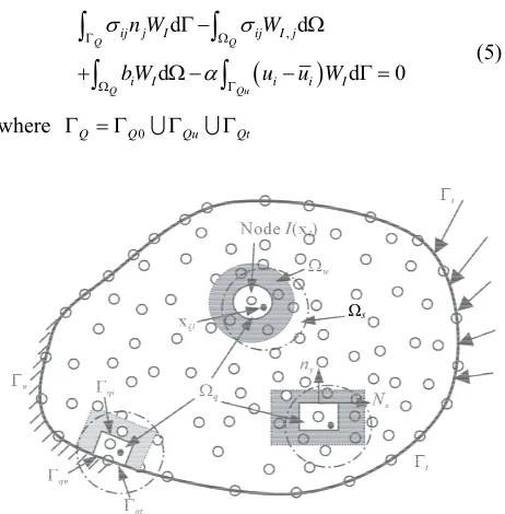
on the essential boundaries.

write a weak form over Q a local quadrature domain (for node I), which may have an arbitrary shape, and contain the point Q



x in question, (see Figure 1). The generalized local weak form of the differential Equations (1) and (3) is obtained by:

 

 









, d d 0 Q Qu

ij j i I

i i I

x b x W u u W

         





(4)

where Q is the local domain of quadrature for node I and Qu is the part of the essential boundary that intersect with the quadrature domain Q.

 

I

W is the weight or test function , K



I

W C 



[12]. The first term in Equation (4) is for the equilibrium (in locally weighted average sense) requirement at node I. The se- cond integral in Equation (4) is the curve integral to enforce the essential boundary conditions, because the MLS shape functions used in MLPG lack the Kronecker delta function property.

 is the penalty factor, Here we use the same penalty factor for all the displacement constraint equations (es- sential boundary conditions) [1]

Generally, in meshfree methods, the representation of field nodes in the domain will be associated to other repartitions of problem domain: influence domain for nodes interpolation, S is the support domain for ac- curacy. For each node W is the weight function do- main, and is the quadrature domain for local inte- gration.

 

Q 

Using the divergence theorem [11] in Equation (4) we obtain:





, d d d d Q Q Q Qu

ij j I ij I j

i I i i I

n W W

bW u u W

              









0

t

(5)

where   Q Q0QuQ

Ωs

Figure 1. The local sub-domains around point and boundaries.

Q

x

0

Q

 : The internal boundary of the quadrature domain

Qt

 : The part of the natural boundary that intersects with the quadrature domain

Qu

 : The part of the essential boundary that intersects with the quadrature domain

When the quadrature domain Q is located entirely within the global domain on Qt and Qu no bound- ary conditions are specified then .



  

0

Q Q

Unlike the Galerkin method, the Petrov-Galerkin me- thod chooses the trial and test functions from different spaces. The weight function



I W

 is purposely selected in such a way that it vanishes on . We can then change the expression of Equation (5): Q0

, d d

d d d

Q Qu Qu

Qt Qu Q

ij I j i I ij j I

i I i I i I

W u W n

t W u W bW

          d W          













 (6)

Witch is the local Petrov-Galerkin weak form. Here we require 0

 

i

u C Q [3,11] and the simplified Pet- rov-Galerkin form is:

, d

Q ij I j Q i I

W b W



    d





 (7) Precedent equations are used to establish the discrete equations for all the nodes whose quadrature domain falls entirely within the problem domain (Equation (7)) and to establish the discrete equations for all the bound- ary nodes or the nodes whose quadrature domain inter- sects with the problem boundary “Equation (6)”.

To approximate the distribution of the function in

S

u

 the support domain over a number of nodes n0.

We shall have the approximant

 

f o u [13]

I h

u x

 

0

 

1 : n h S I I

x u x x u



   



 (8)

where I denote the set of the nodes in the support domain S

 of point xQ.

I

 the MLS shape function for node I that is created using nodes in the support domain S of pointxQ. The discrete system in Equation (6) is given in matrix form:

d d

d d

Q Qu Qu

Qt Qu Q

T

I I

I I

V u W tW

tW u W W b

         d d I I           













(9)

where , , , , 0 0 I x

I I y

I y I x W V W W W          

 is a matrix that collects the

derivatives of the weight functions in Equation (6), and 0 0 I I W W W      

 is the matrix of weight function. The

[image:2.595.58.289.463.698.2]

h d C CL u

   (10) where is the symmetric elasticity tensor of the mate- rial

C





2 2

2 2

1 1 0

1 1 0

0 0 2 1

E E

C E E

E            _   _  _     

Substituting the differential operator

0 0 d x L y y x       _  _ _{   }     ,

and Equation (8) into Equation (10) we obtain:

0

1

n I I I

C B u









(11)

where , , , , 0 0 I x

I I y

I y I x

B     _  _{ }   

 n _



and by using

1 2 2 1 0 0 n n L n n         the tractions of a point x can be written as:

T n

tL (12)

Substituting Equations (8), (11) and (12) into Equation (6), we obtain the discrete systems of linear equations for the node I.

0 1 d d d d d Q Qu Q

Qt Qu Q

n

T

I I I I

I

T

I n I I

I I

V CB W

W L CB u

tW u W W b

          _{   }    _     

 











I d

(13)

That can assembled in matrix form:

0 1 n I I I I

K u f







(14) where nodal stiffness matrix

d d

d

Q Qu

Q

T

I I I I I

T I n I

K V CB W

W L CB

        







  (15)

And nodal force vector with contributions from body forces applied in the problem domain, tractions applied on the natural boundary, as well as the penalty force terms.

d d

Qt Qu Q

I I I I

f tW  u W W b

  



_

 

_

 

_

d (16)

Two independent linear equations can be obtained for each node in the entire problem domain and assembled all these equations to obtain the final global sys-

tem equations:

2n

2n2n 2 1n 2 1n

K _ U _ F _ (17)

To solve the precedent system, the standard Gauss quadrature formula is applied with 16 Gauss points [3,14] for evaluation of boundary and domain integrals in Equa- tions (15) and (16)

3. Numerical Example

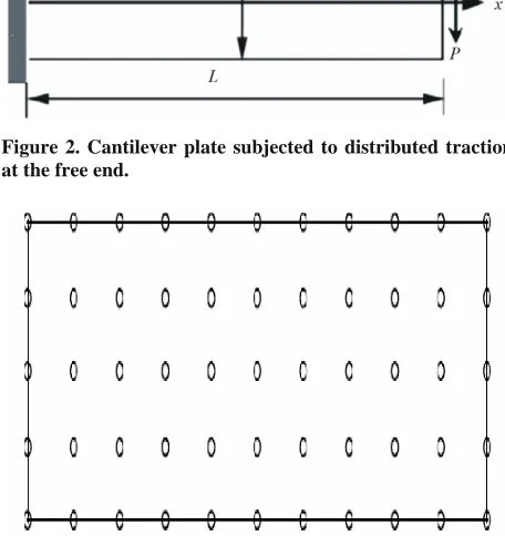
In this section, numerical results are presented for Canti- lever rectangular plate in Figure 2. First we investigate the effects of the size of support or quadrature domains and we examine the numerically convergence of MLPG, then comparisons will be made with the analytic solution [15]

The problem data:

The height of the beam and the length of the beam:

12 m

D

48 m;

L

The thickness of the plat: and Loading (integra- tion of the distributed traction):

unit

P10 N;3

Young’s modulus: _{E 3 10}7_{N m}2 _{and Poisson’s}

ratio:  0.3.

The standard Gaussian quadrature formula is applied with 16 Gauss points, and for MLS approximation linear polynomial basis functions are applied, the cubic spline function is used as the test function for the local

[image:3.595.54.293.81.393.2]

Petrov-Figure 2. Cantilever plate subjected to distributed traction at the free end.

[image:3.595.58.277.426.615.2] [image:3.595.307.535.465.707.2]

Galerkin weak-form. In our numerical calculations we consider many regular distributions of nodes: 55 or 175. To calculate the error energy a background cells is re- quired, then we have varying the number of cell. To ob- tain the distribution of the deflection and stress through the plates, size of quadrature domain and support domain are varied. Nodal configuration for a cantilever plate with 55 nodes (Figure 3) (nodal distance ) and the sizes of Q is defined by: Q

4.8, 3

cx cy

d  d 

Q cI

r d

 

r

where cI

is the nodal spacing near node I and Q is the size of the

local quadrature domain for node I. The sizes of quadra-

ture domains will be, there fore determined by Qx d

 and

Qy

 which are dimensionless coefficients in x and y di-

rections, respectively. For simplicity

Qx Qy Q

   is used. The dimension of the support domain is determined by dssdc and s is the di-

mensionless size of support domain.

[image:4.595.320.524.361.512.2]

4. Discussions

Figure 4 Shows the variation of the effective transverse shear stress xy at different points on vertical of the plate

by varyingx for  s 3 and  Q 1.5. It can be seen

the shear stress distributions on the cross-section at in other sections (xL 4,xL 2,x3 4L and xL).

it’s shown that the shape is identical to that obtained by theoretical analysis ( section xL).

[image:4.595.71.275.537.684.2]

The accuracy is clear for the greater value of field nodes distribution. It is also shown in this figure, on the cross-section the meshless MLPG agree well with those from analytical solution (dashed lines).

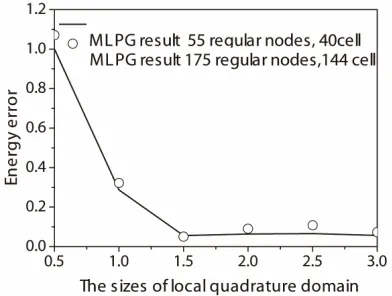
Figure 5 displays the variation of the energy error as a function of the size of the local support domain, for fixed value of Q, a background cells is needed, we take

1.5 Q

  . We note on the figure the effect distribution field nodes number on the result, we take n = 55 and 175

number of cell is nc 40 and 144 respectively.

-6 -4 -2 0 2 4 6

-140 -120 -100 -80 -60 -40 -20 0

S

h

ear stress

y

[image:4.595.323.519.555.703.2]

MLPG result 175node x=L/4 MLPG result 175node x=L/2 MLPG result 175node x=3L/4 MLPG result 175node x=L Analytical result

Figure 4.Shear stress

 

_xy distribution as a function of y for different values of x (xL4,xL 2,x3L

In the case  Q 1.5 For the value of field nodes num-

ber n55 (number of cell is ) the result gives

a greater domain when the value of

40 c n 

:1.85 5

s s

  

can be selected and the method is yet convergent. For n = 175



 Q 1.5



3 s

the domain when accuracy is good in 1.8  our results are comparable to those obtained by other authors [3,5,6].

But in case  Q 2, we have considered n = 175 the

domain of convergence is found to be greater

1.85s3.65.

Figure 6 displays the variation of the energy error as a function of the size of the local quadrature domain, for fixed value of s a background cells used, we take

3 s

  and we choose two values of n = 55 and 175

number of cell is nc 40 and 144 respectively.

For the selected values n the domain when the value of

Q

 can be selected and the method is yet convergent is



1.5Q3 .



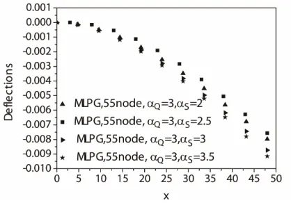
In Figure 7 the deflection results are plotted as func- tion of x and fixed value of  Q 1.5 where y = 0 and by

varying the size of the support domain



 s 2; 2.5;3;3.5



.

the function presents a classical shape It can be seen that

Figure 5. Influence of the _Son energy error for diffe t .

ren distribution nodes numbers

4 and ) ( 175 regular field nodes).



x L

Figure 6. Influence of the _Qon energy-error for two is- rs.

for all values of s and reaches the analytical solution.

fle

[image:5.595.67.276.368.514.2]

The effect of the field distribution number on the de-ction values is presented in Figure 8. For different values of sand Q A Comparison is made with the analytical r ults o eflection (solid line plotted in the Figure 8).

For Q

es f d

2  

en giv

the greater values of nodes numbers n =

175 ev es precision for the greater values of

3.65 s

  (dashed curve). No curve is available for n =

Fo 55.

r the less values of s—we have found in Figure 5 1.85

s

  —two curves plotted for n = 55 and n =

It a

are 175.

lso presented the variation of the defection in the case s3.65,Q2 for n = 55 the curve coincides with that of the analytical results.

5. Conclusion

In conclusion, the size of the local quadrature and sup- port domain affect the accuracy and performance of the MLPG methods and it also show a great influence of the choice of field nodes distribution number. The conver-

[image:5.595.66.275.557.706.2]

Figure 7. Deflections at the central axis at y = 0 of the plate for different values of  S



S2 2 5 3 3 5, . , , .



.

Figure 8. Deflections as a function of x at y = 0, for

, 55 175

t

n and different value of _Sand_Q.

accuracy of MLPG me sti

gence and thod can ll be better

by using a number of appropriate nodes in a large do- main when the support sizing coefficient S can be

chosen and Q is fixed. In our numerical ex ples the

MLPG gives a very close value in comparison with the analytical results.

am

REFERENCES

[1] T. Belyschko, Y. Y. Lu and L. Gu, “Element-Free Galer- kin Methods,” International Journal for Numerical Meth- ods, Vol. 37, No. 2, 1994, pp. 229-256.

doi:10.1201/9781420082104.ch2

[2] S. N. Atluri and S. Shen, “The Meshless Local Petrov-

iu, “Mesh Free Methods, Moving beyond the Fi- for Do-

, H. T. Liu and Z. D.Han, “Meshless Local Galerkin (MLPG) Method,” Tech Science Press, Forsyth, 2002.

[3] G. R. L

nite Element Method,” CRC, Boca Raton, 2003. [4] S. N. Atluri, “The Meshless Method, (MLPG)

main & BIE Discretizations,” Tech Science Press, For- syth, 2004.

[5] S. N. Atluri

Petrov-Galerkin (MLPG) Mixed Collocation Method For Elasticity Problems,” Tech Science Press CMES, Vol. 14, No. 3, 2006, pp. 141-152. doi:10.1152/jn.00885.2006 [6] S. N. Atluri1, Z. D. Hanl and A. M. Rajendran, “A New

esh-

G. Kim, “Analysis of Thin Implementation of the Meshless Finite Volume Method, through the MLPG ‘Mixed Approach’,” Tech Science Press CMES, Vol. 6, No. 6, 2004, pp. 491-513.

[7] J. Sladek, V. Sladek and C. Zhang, “Application of M less Local Petrov-Galerkin (MLPG) Method to Elastody- namic Problems in Continuously Non-Homogeneous Sol- ids,” Computer Modeling in Engineering & Sciences, Vol. 4, No. 6, 2003, pp. 637-648.

[8] S. N. Atluri, J. Y. Cho and H.

Beams, Using the Meshless Local Petrov-Galerkin Me- thod, with Generalized Moving Least Squares Interpola- tions,” Computational Mechanics, Vol. 24, No. 5, 1999, pp. 334-347. doi:10.1007/s004660050456

[9] Y. T. Gu and G. R. Liu, “A Meshless Local Petrov- Galerkin (MLPG) Formulation for Static and Free Vibra- tion Analyses of Thin Plates,” Computer Modeling in En-gineering & Sciences, Vol. 2, No. 4, 2001, pp. 463-476. [10] J. Sladek, V. Sladek, C. Zhang and M. Schanz, “Meshless

Local Petrov-Galerkin Method for Continuously Non-Ho- mogeneous Viscoelastic Solids,” Computational Mecha- nics, Vol. 37, No. 3, 2006, pp. 279-289.

doi:10.1007/s00466-005-0715-0

[11] G. R. Liu and Y. T. Gu, “Meshless Local Petrov-Galerkin (MLPG) Method in Combination with Finite Element and Boundary Element Approaches,” Computational Mecha- nics, Vol. 26, No. 6, 2000, pp. 536-546.

doi:10.1007/s004660000203

117-127. doi:10.1007/s004660050346

[13] T. Belytschko, Y. Krogauz, D. Organ, M. Fleming and P. Krysl, “Meshless Methods: An Overview and Recent De- velopments,” Computer Methods in Applied Mechanics and Engineering, Vol. 139, No. 1, 1996, pp. 3-47. doi:10.1016/S0045-7825(96)01078-X

[14] S. Drapier and R. Fortunée, “Méthodes Numériques

imoshenko and J. N. Goodier, “Theory of Elastic- d’Approximations et de Résolution en Mécaniques,” 2010.

[15] S. P. T