Munich Personal RePEc Archive
Degree of price rigidity in LICs and
implication for monetary policy
ALIDOU, Sahawal
University of Namur, Catholic University of Louvain
June 2014
Online at
https://mpra.ub.uni-muenchen.de/59844/
DEGREE OF PRICE RIGIDITY IN LOW INCOME COUNTRIES : IMPLICATIONS FOR MONETARY POLICY
Sahawal ALIDOU
ABSTRACT
Using semi-aggregate data on price and a methodology based on dummy indicator, we assess
price rigidity in Ghana and discuss its implications for monetary policy. Price features in Ghana are
compared to that of South Africa which is a similar country both in terms of economic structure and
monetary policy framework. Our results suggest higher price rigidity in South Africa than in Ghana.
Therefore, the same monetary policy is likely to have ceteris paribus,
more real effects in South Africa
1 CONTENTS
I) Introduction ... 2
II) Literature review ... 5
1. Price settings in developed countries (USA, EU and Japan) ... 5
2. Price settings in developing countries ... 9
III) Methodology and data set... 13
1. Methods ... 13
2. Data set ... 14
IV) Background on Ghana ... 16
1. Recent socio-economic development ... 16
2. Inflation facts ... 17
V) Results ... 19
1. Indicators of price rigidity ... 19
2. Econometrical analysis’s results ... 22
VI) Discussion: the implications for monetary policy ... 23
VII) Conclusion ... 25
Bibliography ... 26
Appendix 1 : Determination of parameter e ... 29
Appendix 2 : Price rigidity indicators for South Africa ... 30
[image:3.612.66.576.123.457.2]List of tables Table 1 : Frequency of price changes by item for Ghana ... 19
Table 2 : Average amplitude of changes by item for Ghana ... 21
Table 3 : Frequency of price changes by item for South Africa ... 30
Table 4 : Percentage of price increases among price changes for South Africa... 30
Table 5 : Average amplitude of price changes for South Africa... 31
List of figures Figure 1 : Inflation in Ghana over 1990-2013... 18
Figure 3 : Frequency of price increases and decreases for Ghana ... 20
Figure 4 : Amplitude of price changes by month for Ghana ... 21
2 I) INTRODUCTION
Price variations affect agents in the economy in different ways. At the microeconomic level,
consumers tend to reduce their purchasing when prices increase while from producers perspective,
prices increase is an incentive to produce more goods and services. In the same way, changes in both
consumers demand and producers supply are likely to influence prices. Of course, economic agents
do not instantaneously change their behavior in response to price changes and it also take time
before prices adjust in response to changes in demand and supply conditions. The delay of the
responses depends inter alia on agent’s anticipations, wage rigidity, cost of adjustment, structure
of the economy and price-elasticity. One can intuitively think that higher level of savings and
better access to credit allow consumers in developed countries to take more time to adjust to an
increase of prices while consumers in developing countries adjust more rapidly. The literature has
used the terminology of price stickiness to define the duration it takes for price to change or the
frequency at which price change (Carlton, 1986; Bils and Klenow, 2004; Nakamura and Steinsson,
2008; Dhyne et al, 2009).
There are many theories trying to explain price stickiness. It is commonly admitted that
nominal rigidity is determined by wage rigidity, implicit or explicit contracts, menu costs,
attractive prices, fair pricing and costly information1. An important body of literature has been
developing about price settings in developed countries and some notable contributions come
from Bils and Klenow (2004); Nakamura and Steinsson (2008), Klenow and Kryvtsov (2008),
Dhyne, Alvarez and al. (2006)…. In comparison, price settings are quite less known in developing
countries. Mamello Nchake’s (2012) work on Lesotho; Creamer and Rankin’s (2008 and 2012) for
South Africa; Julio and Zarate (2008) for Colombia; Gouvea’s (2007) for Brazil) and Kovanen’s
(2006) for Sierra Leone can be considered as pioneers in such field for developing countries.
Differences in price behavior between developed and developing countries would come at least
from differences in economies structure2. For instance, agriculture still plays a major role in
developing economies whereas it’s not anymore the case in developed economies dominated by
industrial and services sectors. Given that prices of services change far less frequently than others
(see Nakamura and Steinsson (2008), Klenow and Kryvtsov (2008), Dhyne, Alvarez and al. (2006)),
1
See Dhyne et al (2006) and Dhyne et al,(2009)
2Agriculture value added represents 28% of GDP in low income countries in 2012 while it’s only 1% in high income
3 one would expect prices changes to be on average less frequent in developed countries than in
developing one. Finally, price rigidity also depends on market struc ture as models of price
adjustment predict greater frequency of price changes in markets with more competition because
firms therein face more elastic demand (Bils and Klenow, 2004). Given that market failure is
more prevalent in LICs and the nonmarket institutions that ameliorate its consequences are not
very successful in doing so (Stiglitz, 1989), frequency of prices changes in that respect may be
higher in developed countries.
The importance to properly assess price stickiness come from the fact that ‘’most economies
including the developing countries have adopted monetary policy as a means of regulating and
stabilizing the economy, based on the acclaimed short run non-neutrality of money due to sticky
prices and wages, and market imperfections’’ (Urama et al, 2013). Then, price rigidity and speed
of price adjustment are crucial elements to understand business cycle fluctuations and the effects
of monetary policy. Actually, the effects of monetary policy shock on prices and output is very
specific to countries depending on the size of the price rigidity but also on the relative
significance of cost channel effect and negative demand effects3 (Creamer and Rankin, 2008). As
such, price stickiness has several implications for the design of monetary stabilization policy.
That’s probably why monetary authorities focus in general on inflation as a good signal for prices instead of the price level itself. But ‘’inflation may disguise different underlying patterns of price
changes, such as price rigidities, which may cause real effects in the economy. Therefore,
analyzing prices at a unit level4 facilitates an understanding of actual pricing conduct at the most
basic level’’ (Creamer and Rankin, 2008).
Our work is a part of a broad research agenda on Ghana that aims to determine to what
extent models and policies designed for South Africa’s economy can be adapted in Ghana. This
approach is motivated by similarities between the two countries in term of production structure
and monetary policy framework and also the relatively poor quality of data in Ghana. In particular,
we here compare price settings in the two countries to see whether one can assume price in Ghana
to be as stickier as in South Africa. The methodology is inspired from Dhyne, Alvarez and al (2006)
3
As a rising interest rates put upward pressure on prices (firms perspective) and put downward pressure on prices (consumers perspective).
4
4 but given data constraints, we used consumer price indexes instead of micro data on price. Our
results suggest highest price rigidity in South Africa than in Ghana and therefore the need of some
5 II) LITERATURE REVIEW
There are two main ways to investigate price settings. The first consist on ‘’vector
autoregressions (VAR) based on aggregate data (see for example Christiano, Eichenbaum and Evans,
1999) and typically finds stickiness in the aggregate price level’’5. The second way is to exploit
individual level data from survey of firms (Fabiani et al, 2005), or from Producer Price Index
(Vermeulen and al, 2007) or from Consumer Price Index (Bils and Klenow, 2004; Nakamura and
Steinsson; 2008). Former studies using micro data focused on specific wholesale or retail items (see
for instance Carlton, 1986) but recent papers6 deal with larger dataset of products and analyze price
settings both from consumer perspective (CPI) and producer perspective (PPI). According to Dhyne
et al (2009), the most popular approach to explain price rigidity at individual level is the menu cost
model. But studies based on CPI data widely used a dummy indicator to count for changes and
compute frequency of changes (for instance Nakamura and Steinsson,2008 ; Dhyne et al, 2006; Bils
and Klenow, 2004). Also, the methodology has been improving with the distinction between regular
price and temporary price, the role of temporary sales and product substitutions in price changes, the
distinction between state and time pricing, and several transformations of the initial menu cost model
introduced by Barro (1972)7. As this study is based on CPI data, we focus our literature review on
studies at individual level in particular those using CPI data.
1. Price settings in developed countries (USA, EU and Japan)
The work of Bils and Klenow (2004) on price of U.S can be considered as a reference for the
recent body of literature on price features. Using a 1995–97dataset of 350 categories of goods and
services covering about 70% percent of consumer spending and a methodology based on dummy
indicator, they found a median duration of price of 4.3 months. A more detailed dataset8 than that
of Bils and Klenow (2004) and a mixed methodology (dummy and benchmark menu cost model )
allowed Nakamura and Steinsson (2008) to establish the following five facts about price settings in
5
Boivin et al (2007)
6 For instance Nakamura and Steinsson (2008)
7 The menu cost model is based on firm pricing behavior. For further details on methodological evolution, see notably
Klenow and Krystov (2008) Nakamura and Steinsson ( 2008) Dhyne et al (2009) and Kehoe and Midrigan (2010)
8 CPI microdata for 360 products on 1997 and for 270 products on 1998-2005 and microdata of PPI on
6 US. Firstly, temporary sales and product substitutions9 play an important role in generating price
flexibility and price changes are heterogeneous among the products. Secondly, price decreases are
roughly one-third in both consumer prices excluding sales and finished-goods producer prices.
Thirdly, the frequency of price increases covaries quite strongly with the rate of inflation, whereas the
frequency of price decreases and the size of price increases and decreases do not. The fourth feature
is the high seasonality of price rigidity both for consumer and producer prices. Furthermore, prices
are substantially more likely to change in the first quarter than in other quarters of the year. Finally
(fifth feature) they calibrated a model to estimate a hazard function of price changes and found an
upward sloping hazard function for the first months. But this result is not robust because while
changing the model, the hazard function becomes downward sloping.
The results found by Nakamura and Steinsson (2008) are similar to those of Klenow and
Kryvtsov’s (2008)10 who used 1988–2004 US microdata on CPI with also a methodology based on
dummy indicator. For instance, Nakamura and Steinsson found 7.5 months as time-weighted average
of duration of regular prices, including product substitutions. Excluding product substitutions, they
found 8.7 months and for regular prices they found 9.6 months. Klenow and Kryvtsov (2008)
findings are 7.2 months while including substitutions, 8.7 months while excluding substitutions and
9.3 months based on regular prices. Nakamura and Steinsson (2008) findings about the frequency of
price change, the relationship between the frequency of price increases and inflation, and the
seasonality of price changes are also consistent with the results of some important works on price
settings in Europe (Vermeulen et al. (2007); Fabiani et al. (200511)).
For the Euro zone, using a common sample of 50 goods or services of CPI observed
during the January 1996–January 2001 and a methodology based on dummy indicator, Dhyne
et al (2006) found a monthly frequency of price changes of 24.8%, similar to the results in US
(26.1 % from Bils and Klenow, 2004 and 29.3% from Klenow and Kryvstov, 2008). But they
suggested a different way to calculate the duration of the average price spell arguing that inversion
9 Product substitution is particularly important for durable goods and refers to the introduction of new
products. For example seasonally change in clothing products or new model year for cars.
10Their article ‘’State
-dependent or time-dependent pricing: does it matter for recent US. inflation’’ was first published in January 2005 by the National Bureau of Economic Research, WP 11043 and in August 2008 by the Quaterly Journal of Economics
7 of the average frequency of the changes is correct only if prices all have the same expected
duration. Since prices of some products change very infrequently, they compute duration for each
product and then take the average. With this method, prices last on average 13 months in the euro
area and the corresponding figure for the US is 6.7 months. Meaning that the average duration of a
price spell in the euro area is about twice as long as in U.S. So, prices seem to change far less
frequently in the euro area than in the U.S. The differences in frequencies of price adjustment and
durations of price spell between the euro area and the United States seems to be a robust and may
be explain by greater intensity of information and communication technology and greater
competition in retail sector in U.S.
Dhyne et al (2006) also found a substantial variation of the frequency of price changes across
products. For example, prices in the energy sector change very often: 78.0% in a given month while
prices of processed food and non-energy industrial goods change only for 13.7% per month and
9.2 % per month respectively. The lowest incidence of price changes is observed for services.
Those findings support the idea that more labor intensive is a good, less subject to frequent
price adjustments it is, because of wages and contracts rigidity. While goods with relatively
large intermediate inputs experience more frequent price adjustments because of the volatility
of input prices (A´ lvarez and Hernando, 2005).
In the line of Klenow and Kryvtsov (2008) who report that 45% of price changes in US
are decreases, Dhyne et al (2006) found 40% of the changes are price decreases in Euro area.
Another finding is that price changes are greater than the prevailing inflation rate. Price
reductions and price increases have a similar order of magnitude: the average price decrease in
the euro area is 10% while the average price increase is 8.12%. The same pattern is also found
by Klenow and Kryvstov (2008) with U.S. price data: an average price decrease of 14% and an
average price increase of 12.7 %. Otherwise, they established that price changes are not
synchronized across products, even within the same country using Fisher and Konieczny
measure13. Actually, the degree of synchronization of price changes is, except for energy prices,
rather low.
12
The size of price increases and decreases are computed as the difference of logarithms. Thus, during a temporary price cut in which the price returns to its original level, the two successive price changes will be equal in absolute terms.
13
8 Finally, Dhyne et al (2006) assessed the relative importance of different factors on price
changes through an econometrical analysis14. The results suggest that inflation does not significantly
affect the overall frequency of price changes but when running separately price increases and price
decreases, higher inflation increases frequency of price increases and decreases frequency of price
reductions. Similarly, inflation has a positive, but not significant, effect on the size of price
increases, but a negative effect on the size of price decreases. Prices subject to some forms of
regulatory control are found to change considerably less often but the regulatory control variable
does not have a statistically significant impact on the size of price changes.
Using 493 of the 598 item of Japan CPI micro data from 1989 to 2003 and a methodology
based on dummy indicator, Masahiro and Saita (2007), found lower frequency of price change in
Japan than in the U.S and in the Euro area namely is 21.4% per month. But as in U.S and E.U, prices
of good change far more frequently than those of services (31.1% for 4.5%). In line with the results
of Dhyne et al (2006) and A´ lvarez and Hernando (2005), their findings also suggest a negative
correlation between the frequency of price changes and the share of labor costs in the production
costs.
To sum up, both the U.S, the Euro zone and Japan are subject to an important degree of
nominal price stickiness. But prices seem to change less frequently in Japan and in Europe than in
the U.S, suggesting ceteris paribus more real effects of monetary policy in Japan and Euro area and
more nominal effects in the U.S. There is a consensus about monthly price changes frequencies
between 21.4% and 29.3%. However, there are substantial variations of frequency of price changes
from a type of product to another (for example energy and unprocessed food versus service,
non-energy industrials goods and non processed food). Furthermore, there is no evidence of general
downward price rigidity and the degree of synchronization of price changes seems to be low.
14
9 2. Price settings in developing countries
In developing countries, theoretical and empirical works in the field of price settings are spare.
For example, using CPI micro-level prices on 229 products in Lesotho for the period
2002-2009 and a methodology based on dummy indicator, Nchake (2012) found that on average,
39% of prices of food products change every month while the corresponding for non-food
products and services are respectively 33% and 28 %. Pricing is time-dependent mainly because
of weather, the timing of sales, and institutional factors such as changes in regulated prices at
specific periods of the year (for example at the end of the year such that household can afford
more goods for celebrations). On average 44% of prices in rural areas change every month
while the corresponding in urban area is 36%. The implied duration of a price spell is then 2.3
months in rural areas while it is 2.8 months in urban areas. Also, price increases are more
frequent than price decreases and price increases generally follow the overall increase in inflation.
Otherwise, there is a positive and significant correlation between inflation (both current and
previous period inflation) and the frequency of price change in Lesotho.
Using CPI and PPI micro data on the period 2001-2007 and a methodology based on
dummy indicator, Creamer and Rankin (2008 and 201215) have been conducting a broader
research to analyze the implications of price setting behavior for monetary policy in South Africa.
They established stylized facts of price settings in South Africa and provide empirical evidence
about either pricing conduct is state- dependant or time-dependant using time-series regressions.
Furthermore, they introduced micro-founded results about price settings into the open economy
Dynamic Stochastic General Equilibrium (DSGE) model for the South African economy
developed by Steinbach et al. (2009) to compare their results with those obtained from the
DSGE model : the observed prices (micro data evidence) are less sticky than assumed in the
DSGE model16. In details, their main findings are: (i) the frequency of price changes is 17.1%.
Price increases occurred on average more than price decreases (monthly 10.50% for 5.47%) and the
average price duration is 5.0 months; (ii) from CPI perspective, price of goods changes more
frequently (17.0%) than that for services (14.9%). From the PPI micro data, the frequency of
price changes for imported products (23.2%) is higher than for local products (18.8%) and for
15
The paper of 2012 involved also Greg Farell ; South African Reserve Bank Working Paper July 2012 16
10 exported products (18.7%); (iii) the weighted average magnitude of price change is 2.91%. For the
prices that rose, the average magnitude is 12.26% and for the prices that declined, it’s -15.05%. The
econometrical analysis showed a time pricing evidence as there is seasonality in the frequency of
price changes. But the frequency of price changes is also affected by inflation, increases in the repo
rate and increases in the nominal effective exchange rate, denoting state-determined pricing evidence.
With a methodology based on menu-cost model on Nigeria’s data, Urama et al (2013)
conclude on low price rigidity in Nigeria because the cost of non adjustment to a 5% increase in
money supply is too high for firms: price rigidity is optimal decision for firms in Nigeria only when
the menu cost is well above 2.28% of the firm’s revenue.
More generally, results found for developing countries about price facts are the following:
Sierra Leone has the highest average frequency of price change of 51% mainly due to inflation
uncertainty (Kovanen, 2006). In Brazil, the frequency is about 26-37%, exhibiting however a
large degree of product and sector heterogeneity (Gouvea, 2007). In Columbia the frequency of
price changes in a given month is 46.1% (Julio, Zarate and Hernandez, 2008) implying a
stickiness duration of 4.7 months. The results found in Chile are 40% for price changes in a
given month and a synchronization index of 0.437 for price movement. These results, based on
dummy methodology, suggest a huge heterogeneity among developing countries about price
behavior.
The implication of disaggregated price’s rigidity in term of monetary policy is an evolving debate
as it concerns a key assumption of Keynesian-type macroeconomic models that is price stickiness in
the short-run. Bils, Klenow and Kryvtsov (2003) exploited difference in price flexibility across goods
to check through a VAR specification, whether monetary shocks have predicted effects. Their
findings suggest that sticky price models do not represent well U.S economy and monetary policies
based on this assumption do not have the expected effects. However, using also a VAR model based
on quarterly data of federal funds rate, real GDP, GDP deflator, and an index of spot commodity
prices covering the period 1966:Q1 to 2002:Q4, Olivei and Tenreyro (2005) found that monetary
11 shock occurring in the first quarter of the year in USA increases significantly output level and the
response dies out 12 quarters after the shock. Whereas prices respond by declining but at a not
statistically significant level and start rising seven quarters after the shock. When the monetary shock
takes place in the second quarter, the response of output is faster, more sizable and dies out more
quickly (eight quarters after the shock). Then prices start rising faster: three quarters after the shock.
By contrast, the response of output to a monetary policy shock either in the third or in the fourth
quarter is small and insignificant. Here, prices start to increase immediately after the shock. They
explain their findings by wage rigidity features, precisely the seasonality in the flexibility of wage which
Nakamura and Steinsson (2008) linked to seasonality in prices changes. Using a factor-augmented
vector autoregression model (FAVAR) on a panel of 653 monthly series on macroeconomic
indicators, personal consumption expenditure, consumer prices, real consumption and producer
prices covering the period 1976:M1 to 2005:M6 for U.S, Boivin et al (2009) reconciled flexibility of
disaggregated price with price sticky assumption by assessing the relative importance of the
sector-specific and macroeconomic shocks in prices series fluctuations. They found that disaggregated price
fluctuations are driven by sector-specific shocks and remain sticky after monetary shocks. Hence, the implication of micro price’s flexibility in term of monetary policy effectiveness depends on the relative importance of monetary shocks in disaggregated price fluctuations. Moreover, Kehoe and
Midrigan17 (2010) argued that, the changes in price must be decomposed in temporary price changes
and regular price18 changes to get a sharper insight of the link between micro price flexibility and
aggregate price stickiness. The point is that 72% of price changes are temporary and in about 50% of
cases, after the change in a temporary price change, the nominal price returns to its initial nominal
level (which is the old regular price). The frequency of regular price changes is found much smaller at
7% per month (corresponding to an average duration of 14.5 months) and thus price are sticky
overall. Their model takes into account both temporary and regular price and reproduces the main
evidences from micro price data (notably in term of frequency of changes). The key result is that
frequent temporary price changes do not translate in changes of aggregate price and monetary
policies still have real effects notably on output and consumption.
17
They introduced micro evidence from Nakamura and Steinsson’s dataset in a macroeconomic menu cost-model with temporary price which they estimated with a SVAR
18Regular price is determined by the trend of nominal price’s fluctuations and temporary price is the
12 In overall, it’s established in the literature that: (i) prices changes are heterogeneous among
products; (ii) price stickiness varies from rural to urban areas in developing countries, (iii) prices
changes are both prices increases and decreases, (iv) synchronization in price changes is rather low,
(v) it seems to be a positive relationship between inflation and the frequency of price change. In term
of monetary policy implications, basically low rigidity of price implies more nominal effects than real
effects. But this implication is not straightforward as it depends on the relative importance of
sector-specific shocks (Boivin and al, 2009) and on the importance and the features of temporary and
regular prices (Kehoe and Midrigan, 2010). Also, the findings of Olivei and Tenreyro (2005) suggest
13 III) METHODOLOGY AND DATA SET
1. Methods
a) Frequency of price changes
Following Nakamura and Steinnson (2008), Dhyne et al (2006) and Medina et al (2006), the
method is based on dummy indicator to count for price changes. The frequency of price changes is
calculated for each item as the ratio of the number of price changes to the number of valid price
records. Given that we are dealing with monthly price index, we introduce a parameter e in the basic specification to avoid systematic 100% frequency of changes. Let I be the set of items of CPI and let
denote the logarithm of the price index of category i at time t, we define a dummy variable as the
following:
The frequency of price change for variety i is then:
can also be computed for each year.
b) Measurement of the direction of price change
We here simply compute the number of price increases and the number of price decreases
through-out the sample for each item in order to assess that either increases are likely more frequent or the
contrary. We distinguish price increases from price decreases as following :
Decreases:
14
c) Econometrical analysis framework
The aim of this part of the analysis is to check the relative importance of the various variables
which will appear having an influence on the changes in price from the results obtained with points
1, 2 and 3 of the methodology. The frequency of changes for each variety is regressed on the
explanatory variables. Since frequency of price change is a fractional variable (bounded between 0
and 1), linear models are not appropriate. The most common way to deal with this issue in the
literature is to use the log-odds ratio as a linear function and run the regression using
heteroskedasticity-consistent estimation.
where is a set of explanatory variables for the variety i.
The marginal effect of each variable on the frequency is then:
With : average frequency of price change in the sample.
Dhyne et al (2005) discussed alternative specifications and methods to this procedure and
conclude on its consistency. A common explanatory variable used in the literature is inflation. Then,
there is potential endogeneity problem as product inflation appears somehow in and is also
included in the general level of inflation. Dhyne et al (2006) suggested to use an inflation rate variable
computed at a disaggregated sectoral level rather than at a product level to attenuate this problem.
2. Data set
The data used here are monthly price indexes of CPI and its sub-components. Ghana’s CPI
categories are food, food and beverage, non-food, clothing and footwear, household goods,
operations and services and miscellaneous goods and services. The data set comes from the Ghana
Statistical Service and the time span is 1997:M9 to 2013:M7. Food and non-food price indexes are
available only from 2005:M1. The indexes measure every month, the general price level of goods and
services that households acquire for the purpose of consumption, with reference to the price level in
2002, the base year, which has an index of 100. The CPI is calculated on the base of a basket of
goods and services of 242 items. Prices are collected on 40 markets across the country and CPI is
15 in household expenditure patterns displayed by the Ghana Living Standards Survey 5 (realized in
2005-2006) and national accounts. The new basket will comprise 272 commodities and data will be
collected on 42 markets. Also, new weights will be assigned to the commodities to reflect their
relative importance in current household consumption.
The data for South Africa have been gathered from the website of South Africa Statistical
Agency. The data set covers the period 2002M1-2013M12 with 15 sub-components of CPI weighted
according to the Income and Expenditure Survey of 2010-2011. We made some little computations
16 IV) BACKGROUND ON GHANA
1. Recent socio-economic development
Ghana is a located along the Gulf of Guinea in West Africa. It is member of the main
economic integration organizations of the region namely the ECOWAS (Economic Community
Of West African States) and the WAMZ (which a step monetary union formed by Ghana,
Nigeria, Guinea, Gambia, and Sierra Leone that will merge later on with West African Economic
and Monetary Union). Ghana has experienced strong GDP growth over the last 20 years with
acceleration in 2008-2012 (notably a growth rate of 1519% in 2011) due to investment in oil
extraction. As a result, Ghana reached lower middle-income status with the challenge to sustain
improvements in growth. However the economy has not undertaken strong diversification.
Although declining, an important share of GDP comes from agriculture (32% in 2009 and 23%
in 2012; World Bank Indicators) while the informal sector still plays a major role in the economy
and remains the main source of employment and job creation (IMF country report, June 2013).
Tax revenues increased from 11.1% of GDP in 2009 to 14.5% in 2012 following Ghana
Revenue Authority reforms and revenue-enhancing measures. Current Account Balance remains
negative over 2004-2013 and even deteriorates from (-3.9% of GDP in 2004 to -14.4% in 2013)
and the Public debt increased from 45.7% of GDP in 2010 to 50.2% in 2012 mainly because of
weaker external outlook and fiscal slippages in 2012 (African Economy Outlook, Report on
Ghana, 2013).
The monetary policy in Ghana is characterized by a shift from a monetary targeting during
the period 1992-2002 to an inflation targeting formally20 announced in 2007, the same year of a
currency redomination. Also, a limit has been put on government’s borrowing in any fiscal year
to tackle the issue of fiscal dominance. An evaluation of these changes concluded that the
inflation targeting regime has been successful in bringing inflation down. Indeed, headline
inflation reduced from 20% percent levels in 2004 to 10.7% by end-2010 and the interest rate
channel, a key channel of inflation targeting policy, seems to function in a standard way.
However, the evaluation stresses that the monetary framework must be more transparent and
more accountable (IMF country report, June 2013).
19
World Bank Indicator, WDI tables
17 The strong economic performances have been followed by improvements in standards of
living. Indeed, Ghana’s Human Development Index ranking is 135th out of 183 countries in 2012
and the incidence of extreme poverty reduced from 52% in 1991 to 28.3% in 2006. The net
school enrolment rate increased from 59% in 2001-2002 to 81.7% in 2011-2012. Child mortality
fell from 111 to 78 per thousand live births between 2003 and 2011 and maternal mortality ratio
declined from 206 to 164 per one hundred thousand live births between 1990 and 2010 (Ghana
MDG Report, 2012).
In the medium-term the three main challenges for Ghana economy are : (i) restore
macroeconomic and debt sustainability by fiscal consolidation ; (ii) economic diversification to
create a robust job-creating manufacturing sector; (iii) social inclusion to ensure that the benefits
of growth are widely shared and to build a workforce ready to take on higher-skilled jobs (IMF
country report, June 2013).
2. Inflation facts
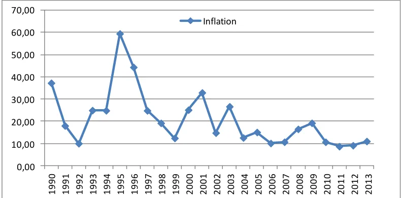
The period 1990-2002 is characterized by a highly volatile inflation with a peak at almost 60% in
1995. This situation is due to strong fiscal dominance in which persistent fiscal deficits were financed
largely by monetary accommodation (generating high inflation tax). As a result, money had an
instable and high velocity (hot potatoes phenomenon) and inflation expectations became difficult or
impossible to predict (Monetary policy framework in Ghana, Bank of Ghana, 2012). In 2002, the
monetary framework is completely changed and the new one is designed to lower inflation and
ensure exchange rate stability, through increased coordination with fiscal policy. More precisely, the
monetary policy shift to an inflation targeting regime and fiscal dominance has been significantly
reduced. Consequently, inflation progressively decreased but with a transition period from 2002 to
2009. As the new monetary framework gains in credibility, inflation is stabilized around 10% since
18 Figure 1 : Inflation in Ghana over 1990-2013
0,00 10,00 20,00 30,00 40,00 50,00 60,00 70,00
1990 1991 1992 1993 1994 1995 1996 1997 1998 1999 2000 2001 2002 2003 2004 2005 2006 2007 2008 2009 2010 2011 2012 2013
Inflation
19 V) RESULTS
1. Indicators of price rigidity
a) Frequency of changes
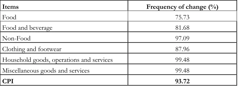
The average frequency of changes is 93.72% meaning that prices indexes change almost every
month in a year. Food index display the lowest frequency of change (75.73%) while Household
goods, operations and services index and Miscellaneous goods and services index have the highest
one (99.48%) [Table 1]. The corresponding figure for South Africa is an average frequency of price
changes of 61.81%. The lowest frequency of changes is that of Education (8.33%) and the highest is
that of Transport (84.03%) [Table 3].
The level of disaggregation is not the same from Ghana CPI to that of South Africa but they
have two common items21 (Food and Clothing and footwear). For both, frequency of changes is
higher in Ghana. Indeed, Food index changes 8 months out of 12 (i.e a frequency of changes of
68.06%) in South Africa while it changes 9 months out of 12 in Ghana. Meanwhile the frequency of
[image:21.612.70.462.434.576.2]changes of Clothing and footwear is 87.96% in Ghana and 56.25% and South Africa.
Table 1 : Frequency of price changes by item for Ghana
Items Frequency of change (%)
Food 75.73
Food and beverage 81.68
Non-Food 97.09
Clothing and footwear 87.96
Household goods, operations and services 99.48
Miscellaneous goods and services 99.48
CPI 93.72
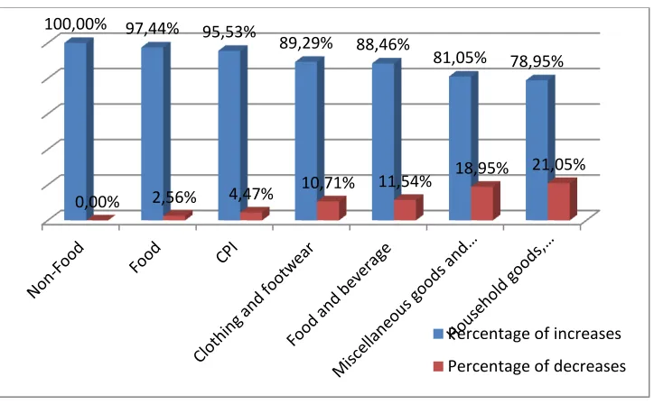
b) Direction of price changes
The price changes are far more increases than decreases in Ghana. Less than 5% of changes
are decreases for the CPI and 100% of changes are increases for non-food index. However,
21
20 decreases represent 21% of changes of Household goods, operations and services index and
[image:22.612.109.471.143.367.2]almost 19% for Miscellaneous goods and services index [Figure 3].
Figure 2 : Frequency of price increases and decreases for Ghana
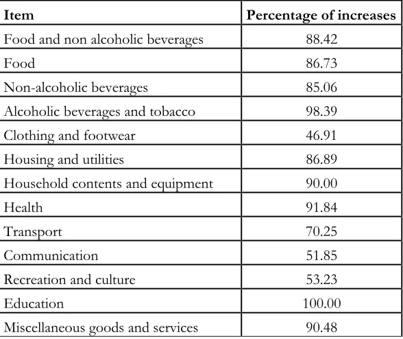
The global figure for South Africa is pretty much the same: changes in price are far more
increases and less than 5% of changes are decreases for the CPI. But for Clothing and footwear,
Communication and Recreation and culture changes are increases and decreases almost in the same
proportion [Table 4].
c) Amplitude of price changes
For Ghana, the CPI average amplitude of changes is 1.38%, the lowest average amplitude is
that of Food and the highest is that of Miscellaneous goods and services [Table 2]. The average
amplitudes of changes are quite lower of South Africa in comparison to those of Ghana. The CPI
average amplitude of changes is 0.21%, the highest value is 0.37% (Transport) and the lowest is
0.17% (Household contents and equipment) [Table 5]. 100,00% 97,44% 95,53%
89,29% 88,46%
81,05% 78,95%
0,00% 2,56% 4,47%
10,71% 11,54% 18,95%
21,05%
Percentage of increases
21 Table 2 : Average amplitude of changes by item for Ghana
Items
Average amplitude of price changes (%)
Food 0.74
Food and beverage 1.37
Non-Food 1.13
Clothing and footwear 1.39
Household goods, operations and services 1.55
Miscellaneous goods and services 1.72
CPI 1.38
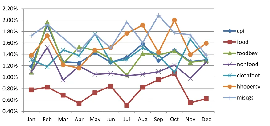
Especially in Ghana, the average amplitudes of changes are more important in February and
in October for CPI while the peaks for Miscellaneous goods and services occur in September and
November. July seems to be the month in which the amplitude of changes is generally low for all
categories in particular for food index. The specific pattern of foods indexes reflects the seasonality
in agricultural production: the new crops come in July and there is a minor crop in November. Also,
the increase of the amplitude for almost all the items (5 out of 7) in December may reflect usual
holiday season’s inflation [Figure 4].
Figure 3 : Amplitude of price changes by month for Ghana
0,40% 0,60% 0,80% 1,00% 1,20% 1,40% 1,60% 1,80% 2,00% 2,20%
Jan Feb Mar Apr May Jun Jui Aug Sep Oct Nov Dec
[image:23.612.75.513.447.652.2]22 Altogether, the average frequency of changes is higher in Ghana than in South Africa. The
changes are far more increases than decreases in both countries but the average amplitudes of
changes are higher in Ghana. Also, there is a relatively important heterogeneity in frequency of
changes across items in South Africa (from 8.33% for Education to 84.03% for Transport) while in
Ghana frequencies are concentrate in the interval 75-100%. Overall, the results suggest that price
change less frequently in South Africa than in Ghana implying a lower rigidity of price in Ghana.
2. Econometrical analysis’s results
The econometrical analysis is done with Ghana’s data. We used yearly frequency of changes of
each item in a panel data approach. We ran both fixed effects and random effects models and check
after their quality with a Hausman’s test. We reported below the results of random effect model
which appears to be better after the test.
Number of obs = 98 Number of groups = 7 Wald chi2(1) = 8.00 Prob > chi2 = 0.0047 Hausman Test
Prob>chi2 = 0.8299
Dependant variable: log (fi/1-fi)
Variable Coef Std. Err. z-statistic P>|z| [95% Conf. Interval] inflation .0135678 .0047971 2.83 0.005*** .0041657 .02297 _cons .5445077 .0914795 5.95 0.000 *** .3652112 .7238043
*** Significant at 1% ** Significant at 5% * Significant at 10%
The correlation coefficient between the frequency of price change and inflation is positive and
significant in line with the findings of Bils and Klenow (2004) and Nchake (2013). The results
suggest that prices change more frequently in situation of higher inflation. This result is consistent
with more frequent renegotiations of wages in inflationary conditions particularly in economies with
important informal sector like Ghana (see footnote 22). It is also consistent with the fact that price
23 VI) DISCUSSION: THE IMPLICATIONS FOR MONETARY POLICY
The main concern of the discussion is how effective can be a monetary policy given the level of
price rigidity. Our results suggest a high frequency of price adjustment in Ghana and therefore a low
rigidity of price. The first implication for monetary policy is that it may have more nominal effects
than real effects. Also, we found higher price rigidity in South Africa, suggesting that the same
monetary policy will have ceteris paribus more nominal effects in Ghana and more real effects in
South Africa.
More nominal effects of monetary policy can be both good and bad news depending on the
main objective of the monetary policy. Indeed when monetary policy targets nominal variable such as
inflation or nominal exchange rate, lower rigidity is an advantage but when targets are real output and
employment, low rigidity appears to be a disadvantage. As in Ghana, the main objective of monetary
policy is to achieve lower inflation and ensure exchange rate stability, low rigidity of price improves
effectiveness of monetary policy. Indeed, price may quickly respond to a contractionary monetary
policy and negative effects on real variables may be low. In line with this interpretation, inflation
targeting monetary framework adopted by Bank of Ghana in 2007 resulted in a progressively
decrease of inflation in Ghana.
But low rigidity of price reduces the effectiveness of monetary policy to overcome demand
shocks. For instance in case of negative demand shock, a depreciation of exchange rate to stimulate
demand will quickly translate into higher price and an upward shift of supply curve. Therefore, the
monetary policy would have less effect on output. In this respect, Al Hajj et al (2013) concluded that
to be fully effective in adjusting to a negative demand shock, monetary policy needs to be supported
by fiscal policy in Ghana while in South Africa, monetary policy alone is enough. In case of positive
demand shock with inflationary pressure, a rise of interest rate to reduce demand will also quickly
translate into high level of price and higher nominal wages22 that would sustain the inflationary
bubble and result also in less effect on aggregate demand.
Moreover, since May 2013 Ghana has been facing an increasing monthly inflation (from 11.3%
in May 2013 to 14% in March 2014, Ghana Statistical Service), casting doubt on the nominal effects
22
24 and the effectiveness of the inflation targeting monetary policy in a context of low rigidity of prices.
But as highlighted by Boivin and al (2009) and Kehoe and Midrigan (2010) the effectiveness of
monetary policies in a context of flexible disaggregated price depends on the relative importance of
sector-specific shocks on disaggregated prices and on the importance and the features of temporary
and regular prices.
Hence, questions are: (i) how do monetary shocks affect disaggregated prices in Ghana and (ii) is
there evidence of temporary and regular pricing in Ghana and what are their features? In terms of
comparison between South Africa and Ghana, lower rigidity of price in Ghana suggests that one
should be careful when trying to adapt macroeconomic models and economic policies designed for
25 VII) CONCLUSION
To properly assess price rigidity using CPI, micro data on price is needed. In this work, we try to
overcome the lack of such data by using price indexes of CPI’s items and introducing a parameter in
the method described in Medina et al (2007). Our results suggest lower rigidity of price and lower
heterogeneity in frequency of changes across items in Ghana in comparison to South Africa.
Basically, the implication of low rigidity of price in Ghana is that monetary policy has more nominal
effects than real effects and will be less effective to adjust to demand shock notably. Moreover, one
would start doubting even on the nominal effects of monetary policy in Ghana as the country is
experiencing higher monthly inflation since almost one year despite an inflation targeting monetary
framework. However, further studies are needed additionally to this work before strong conclusions
can be drawn about monetary policy effectiveness in Ghana. For instance: (i) a detailed analysis of
price settings with micro data on price; (ii) a decomposition of price changes in temporary and
regular prices changes and (iii) a VAR estimation to assess the impact of monetary shocks and sector
26
B
IBLIOGRAPHYAl Hajj F., Dufrénot G., Sugimoto K. and Wolf R., ‘’Reactions to Shocks and Monetary Policy Regimes: Inflation Targeting Versus Flexible Currency Board in Ghana, South Africa and the WAEMU’’, William Davidson Institute Working Paper Number 1062, November 2013
Aucremanne L. and Dhyne E., ‘’Time-dependent versus state-dependent pricing : a panel data approach to the determinants of belgian consumer price changes’’, European Central Bank, Working paper series no. 462 / march 2005
Bils M. and Klenow P., ‘’ Some evidences on the importance of sticky prices’’, Journal of Political Economy, 2004, vol. 112, no. 5, University of Chicago.
Bils M., Klenow P. and Kryvtsov O., ‘’ Price sticky and monetary policy shocks ’’, Federal Reserve of Minneapolis Quarterly Review, Vol 27, N° 1, Winter 2003, pp. 2-9
Boivin J., Giannoni M. and Mihov I., ‘’ Sticky prices and monetary policy: evidence from
disaggregated U.S data’’, American Economic Review, 2009, 99:1, 350-384.
Creamer K., Farrell G. and Rankin N., ‘’ What can price-level data can tell us about pricing conduct
in South Africa?’’, South African Reserve Bank Working Paper, July 2012
Creamer K. and Rankin N., ‘’Price settings in South Africa 2001-2008- stylized facts using consumer
price micro data’’, University of the Witwatersrand, October 2008
Dias D. A., Robalo C., Marques P., Neves D. and J.M.C.Santos Silva ‘’On the Fisher-Konieczny
index of price changes synchronization’’, Banco de Portugal, Economic Research Department Working Paper 7-04 June 2004
Dhyne E., Alvarez L., Le Bihan H., Veronese G., Dias D., Hoffmann J., Jonker N., Lünnemann P., Rumler F. and Vilmunen J, ‘’Price Changes in the Euro Area and the United States: Some Facts from Individual Consumer Price Data’’, Journal of Economic Perspectives—Volume 20, Number 2— Spring 2006 —Pages 171–192
Dhyne E., Alvarez L., Le Bihan H., Veronese G., Dias D., Hoffmann J., Jonker N., Lünnemann P., Rumler F. and Vilmunen J, ‘’Price settings in the Euro area: some stylized facts from individual
consumer price data’’, European Central Bank, Working paper series no. 524 / September 2005
27 Fabiani S., Gattulli A., Sabbatini R. and Veronese G., ‘’Consumer price setting in Italy’’, Banca
d’Italia Working Paper Number 556 - June 2005
Gouvea S., ‘’Price rigidiy in Brazil: Evidence from CPI micro data’’, Banco Central do Brasil, Working Papers Series 143, September 2007
Higo M.and Saita Y., ‘’Price Setting in Japan:Evidence from CPI Micro Data’’, Bank of Japan No.07 -E-20, August 2007
Julio J-M., Zárate H. and Hernández D., ‘’The Stickiness of Colombian Consumer Prices’’, Borradores de Economia, Num 578 2009
Kehoe P. and Midrigan V., ‘’Prices are sticky after all’’, Federal Reserve Bank of Minneapolis, Research Department Staff Report, 413, September 2010
Klenow K. and Kryvtsov O., ‘’State-dependant or time dependant pricing: does it matter for recent
U.S inflation?’’, The Quarterly Journal of Economics, August 2008 and Manuscript. Stanford, Calif.: Stanford Univ., Dept. Econ., 2004
Kovanen A., ‘’Why do prices in Sierra Leone change so often? A case study using micro-level price data’’, WP/06/53, IMF Working Paper, February 2006.
Mamello Nchake, ‘’Price setting behaviour and product inflation in Lesotho’’, University of Cape
Town, South Africa, 2012
Medina J-P., Rappoport D. and Soto C., ‘’ dynamics of price adjustments:evidence from micro level
data for Chile’’, Central Bank of Chile Working Papers N° 432, Octubre 2007
Nakamura E. and Steinsson J., ‘’five facts about prices: a reevaluation of menu cost models’’, The Quarterly Journal of Economics, November 2008
Olivei G. and Tenreyro S., ‘’The timing of monetary policy shocks’’, The American Economic Review, June 2007 vol. 97 no. 3
Steinbach R., Mathuloe P. and Smit B., ‘’An open economy New Keynesian DSGE model of the South African economy’’, South African Reserve Bank Working Paper, April 2009
28 Urama N.E., Oduh M.O., Nwosu E., Odo A.C., ‘’Price Rigidity and Monetary Non-Neutrality in Developing Countries: Evidence from Nigeria’’, International Journal of Economics and Financial Issues
Vol. 3, No. 2, 2013, pp.525-536
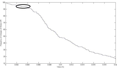
29 Appendix 1 : Determination of parameter e
The parameter e is determined by the checking whether there is a stagnation of the frequency
of CPI for some particular value e. We set the maximum value for e at 2% which is the inflation target of U.S Federal Reserve and European Central Bank as well. This reference value is interpreted
as the highest variation of price one can still interpret as price stability and absence of change.
The function of frequency of change of CPI has a downward slope in line with the fact that
highest value of parameter e reduces frequency of changes. However, one can see a kind of
concentration of frequency of change around the value 0.003 of e. We take advantage of this stability
[image:31.612.74.546.294.573.2]to argue that 0.003 may be the best value to compute the indicators of price rigidity.
30 Appendix 2 : Price rigidity indicators for South Africa
Table 3 : Frequency of price changes by item for South Africa
Item Frequency of price changes (%)
Food and non alcoholic beverages 65.97
Food 68.06
Non-alcoholic beverages 60.42
Alcoholic beverages and tobacco 43.06
Clothing and footwear 56.25
Housing and utilities 42.36
Household contents and equipment 41.67
Health 34.03
Transport 84.03
Communication 18.75
Recreation and culture 43.06
Education 8.33
Miscellaneous goods and services 43.75
Processed good 63.89
Unprocessed 76.39
CPI 61.81
Table 4 : Percentage of price increases among price changes for South Africa
Item Percentage of increases
Food and non alcoholic beverages 88.42
Food 86.73
Non-alcoholic beverages 85.06
Alcoholic beverages and tobacco 98.39
Clothing and footwear 46.91
Housing and utilities 86.89
Household contents and equipment 90.00
Health 91.84
Transport 70.25
Communication 51.85
Recreation and culture 53.23
Education 100.00
[image:32.612.71.365.463.710.2]31
Processed good 93.48
Unprocessed 75.45
[image:33.612.73.367.72.124.2]CPI 95.51
Table 5 : Average amplitude of price changes for South Africa
Item Average amplitude of price changes (%)
Food and non alcoholic beverages 0.29
Food 0.31
Non-alcoholic beverages 0.28
Alcoholic beverages and tobacco 0.31
Clothing and footwear 0.26
Housing and utilities 0.33
Household contents and equipment 0.17
Health 0.25
Transport 0.37
Communication 0.20
Recreation and culture 0.20
Education 0.26
Miscellaneous goods and services 0.21
Processed good 0.29
Unprocessed 0.40