Multiple solutions of steady-state Poisson-Nernst-Planck equations with steric effects

equations with steric effects

Tai-Chia Lin

Bob Eisenberg

Abstract

Experiments measuring currents through single protein channels show unstable currents. Channels switch between ’open’ or ’closed’ states in a spontaneous stochastic process called gating. Currents are either (nearly) zero or at a definite level, characteristic of each type of protein, independent of time, once the channel is open. The steady state Poisson-Nernst-Planck equations with steric effects (PNP-steric equations) describe steady current through the open channel quite well, in a wide variety of conditions. Here we study the existence of multiple solutions of steady state PNP-steric equations to see if they themselves, without modification or augmentation, can describe two levels of current. We prove that there are two steady state solutions of PNP-steric equations for (a) three types of ion species (two types of cations and one type of anion) with a positive constant permanent charge, and (b) four types of ion species (two types of cations and their counter-ions) with a constant permanent charge but no sign condition. The excess currents (due to steric effects) associated with these two steady state solutions are derived and expressed as two distinct formulas. Our results indicate that PNP-steric equations may become a useful model to study spontaneous gating of ion channels. Spontaneous gating is thought to involve small structural changes in the channel protein that perhaps produce large changes in the profiles of free energy that determine ion flow. Gating is known to be modulated by external structures. Both can be included in future extensions of our present analysis.

Keywords: multiple solutions, excess currents, PNP-steric equations

1

Introduction

The Poisson-Nernst-Planck (PNP) equations, a well-known model of ion transport, play a crucial role in the study of many physical and biological phenomena (cf. [3, 4, 7, 8, 12, 14, 16, 17, 31, 38, 39, 43, 47]). Such an important model can be represented by



       

       

∂ci

∂t +∇ ·J P N P

i = 0, i= 1,· · · , N ,

−JP N P i =Di

∇ci+_kz_Bie_Tci∇φ

,

−∇ ·(ε∇φ) =ρ0+

N

P

i=1

zieci

(1.1)

whereN is the number of ion species,ciis the distribution function, JiP N P is the flux density,Di

is the diffusion constant, andziis the valence of theith ion species, respectively. Besides,φis the

electrostatic potential, ε is the dielectric constant,ρ0 is the permanent (fixed) charge density of

the system,kB is the Boltzmann constant,T is the absolute temperature andeis the elementary

charge. Due to ionic sizes, steric repulsion may appear in crowded ions of several biological systems like DNAs, ribosomes and ion channels. When ions are crowded in a narrow channel, the PNP

∗_{Institute of Applied Mathematical Sciences, Center for Advanced Study in Theoretical Sciences (CASTS),}

National Taiwan University, No.1, Sec.4, Roosevelt Road, Taipei 106, Taiwan, email:[email protected]

†_{Department of Molecular Biophysics & Physiology Rush Medical Center, 1653 West Congress, Parkway, Chicago,}

IL 60612, USA, email: [email protected]

1

equations become unreliable because the ion-size effect becomes important, but the PNP equations represent ions as point particles without size (cf. [1, 5, 20, 21, 27, 32, 35, 45]).

To include ion size effects, Eisenberg and Liu modified PNP equations into a complicated system of differential-integral equations with singular integrals that simulate successfully the selectivity of important types of calcium and sodium ion channels (cf. [29]). However, the singular integrals form an extremely singular kernel because of the Lennard-Jones (LJ) potential. Numerical efficiency and theoretical analysis disappear when forced to deal with such singularities (cf. [19, 30]). To simplify the model, we truncate the (spatial) frequency range of the LJ potential, find a simpler energy functional from the leading order terms of the energy expansion with suitable scales. We derive the Poisson-Nernst-Planck equations with steric effects called PNP-steric equations (cf. [36])

∂ci

∂t +∇ ·Ji= 0, i= 1,· · ·, N , (1.2)

− ∇ ·(ε∇φ) =ρ0+

N

X

i=1

zieci, (1.3)

where fluxJi is

Ji=−Di∇ci−

Dici

kBT

zie∇φ−

Dici

kBT N

X

j=1

gij∇cj, (1.4)

and gij = gji ∼ ij(ai+aj)

12

is a nonnegative constant depending on ion radii ai, aj and the

energy coupling constant ij of the i-th and j-th species ions, respectively (cf. [26]). Note that

equations (1.2)-(1.4) can be regarded as a system of reaction-diffusion equations with nonlinear cross-diffusion terms being similar to [9]. Amazingly, these equations are an effective model to simulate the selectivity of ion channels (cf. [26]).

Comparing (1.4) with JP N P

i in (1.1), the excess flux Jiex =Ji−JiP N P due to steric effects of

ion speciesiis

−Jiex =

1 kBT

Dici∇µexi and µ ex i =

N

X

j=1

gijcj

whereµex i =

N

P

j=1

gijcj is the excess chemical potential of ion speciesidue to steric effects.

Conse-quently, the excess currentIex₌ PN

i=1

zieJiex due to steric effects becomes

Iex =−

N

X

i,j=1

zie

kBT

Digijci∇cj. (1.5)

We shall use the formula (1.5) to calculate the excess currents for multiple solutions of the 1D steady-state PNP-steric equations. We are motivated by the hope–but cannot dare expect–that one solution will correspond to a closed state and the other to an open state, as found in experiments [15] and in simulations [33]. Of course, the current measured through the open state corresponds to the total current, not just the excess currents.

For simplicity, we consider domain as a 1D interval (−1,1) for (1.2)-(1.4) and set Ji = 0,

i= 1,· · ·, N to get the steady-state PNP-steric equations. Then by (1.4),

d dx



lnci+

zie

kBT

φ+ 1 kBT

N

X

j=1

gijcj



= 0 forx∈(−1,1), i= 1,· · ·, N ,

which can be satisfied if

lnci+

zie

kBT

φ+ 1 kBT

N

X

j=1

gijcj = 0 for i= 1,· · · , N , (1.6)

holds true. Let ˜φ = _ke

BTφ and ˜gij =

1

kBTgij for i, j = 1,· · ·, N. Then (1.3) and (1.6) can be

transformed into

lnci+ziφ˜+ N

X

j=1

˜

gijcj= 0 for i= 1,· · ·, N, (1.7)

and

−ε˜φ˜xx= ˜ρ0+

N

X

i=1

zici for x∈(−1,1), (1.8)

where ˜ε= kBT

e2 ε and ˜ρ0= 1_eρ0. For notational convenience, we may remove tilde (∼) and denote

(1.7) and (1.8) as

lnci+ziφ+ N

X

j=1

gijcj= 0 for i= 1,· · ·, N, (1.9)

and

−εφxx=ρ0+

N

X

i=1

zici for x∈(−1,1). (1.10)

Equations like (1.9) have been used to interpret bioelectric phenomena in many papers since they were adopted by Hodgkin, Huxley, and Cole (cf. [13, 28]). Here we consider the following boundary condition given by

φ(1) +ηεφ0(1) =φ0(1) and φ(−1)−ηεφ0(−1) =φ0(−1), (1.11)

whereφ0(1), φ0(−1) are constants andηεis a non-negative constant. Hereφ0(±1) andφ(±1) are

the extrachannel and intrachannel electrostatic potentials at the channel boundaries, respectively. The coefficient ηε ∼ _εε_m0 is governed by the ratio of ε0 the dielectric constant of the electrolyte

solution andεmthe dielectric constant of the membrane (cf [48]). Note that (1.11) is of the Robin

boundary condition if ηε > 0; and of the Dirichlet boundary condition if ηε = 0. The Robin

boundary condition includes polarization (e.g. dielectric) charges in the bath and/or electrodes which the Dirichlet boundary condition does not. Such charges, induced by and dependent on the electric field play a prominent role in the art of real experiments, because they are important determinants of the background noise and stability of high speed recordings. The theoretical reasons for these practical realities have not been investigated to the best of our knowledge.

As N = 2, the existence, uniqueness and the solution’s asymptotic behavior of (1.9)-(1.11) are investigated under non-symmetry breaking condition 0≤g12 =g21 ≤

√

g11g22 which implies

that solution (c1, c2) of (1.9) is uniquely determined by φ (cf. [34]). Hence (1.9) and (1.10) can

be reduced to a single differential equation of φ. However, as the symmetry breaking condition g12=g21>

√

g11g22 holds true, solution (c1, c2) of (1.9) may not be uniquely determined byφ. In

Section 2, we introduce new variablesξ,Σ and transform (1.9) into a quadratic polynomial which can be solved precisely to get explicit formulas and represent two branches of solution curves. Using these explicit formulas, we can then define biological conductance (for that condition) as the biologists do and perform the comparison using formulas like (1.12)-(1.15). Note that the symbolg is used for conductance (units siemens) in biology and this is not equivalent to ourgij. In this paper,

we want to study multiple solutions of (1.9)-(1.11) for the cases ofN = 3,4, andg12=g21, g34=g43

sufficiently large such that symmetry breaking conditiong12=g21>

√

g11g22, g34=g43>

√ g33g44

1.1

Main Results

System (1.9) can be regarded as a coupled system of algebraic equations. Because gij = 0 for

i, j= 1,· · · , N, a solution of system (1.9) can be expressed asci=e−ziφfori= 1,· · ·, N. However,

it seems impossible to solve system (1.9) explicitly for the general case ofgij >0 fori, j= 1,· · ·, N.

To overcome such difficulty, we may set N = 2, z2 = −z1 = q ≥ 1, g11 = g22 = g > 0, and

introduce new variablesξ=c1c2 and Σ =c1+c2. Then (1.9) can be transformed into a quadratic

polynomial that can be solved explicitly (see Section 2). Forg12=g21=zlarge (see Theorem 2.4

in Section 2), system (1.9) has two branches of solutions (c1, c2) = (c1(ΣA1(φ)), c2(ΣA1(φ))) and

(c1, c2) = (c1(ΣB1(φ)), c2(ΣB1(φ))) such that (c1−c2)◦ΣA1 : [−φA,c,∞)→Rand (c1−c2)◦ΣB1:

(−∞, φA,c] →Rare monotone increasing functions to φ, where φA,c >0 is a constant, ΣA1 and

ΣB1 are two functions satisfying

(c1−c2)◦ΣA1(−φA,c) = (c1−c2)(Σc)>0,

(c1−c2)◦ΣB1(φA,c) =−(c1−c2)(Σc)<0,

lim

φ→∞(c1−c2)◦ΣA1(φ) =∞ and φ→−∞lim (c1−c2)◦ΣB1(φ) =−∞.

Here◦denotes the function (c1−c2) acting on the function ΣA1(φ), i.e., the function composition

andgc is the positive constant defined in Proposition 2.2. Besides,φA,c satisfiesφA,c→+∞and

(c1−c2)(Σc)→0 asz→+∞and g >0 is fixed. Hence (1.9) and (1.10) can be decomposed into

two differential equations like (3.6) and (3.7) but they can not have uniformly bounded solutions to ε > 0 (see Lemma 4.5). This fact motivates us to add one extra species c3 and assume that

N = 3, g12 = g21 = z is sufficiently large, g11 = g22 = g > 0, z2 = −z1 = q ≥ 1, z3 > 0,

gi3=g3i= 0,i= 1,2,3 (which implies c3=e−z3φ). Then (1.9) and (1.10) may be reduced to two

differential equations (3.6) and (3.7) having uniformly bounded solutions, respectively. This may provide multiple solutions of (1.9)-(1.11).

Natural biological solutions always contain at least three species (sodium, potassium, and chloride, and usually calcium). Experiments are often done, however, with just two species (say sodium chloride) along with traces of hydrogen ion, and perhaps other contaminants. Gating occurs in simplified unnatural situations and so we hope to study mathematical solutions in corresponding situations in a separate paper.

Now we state the main result of this paper as follows:

Theorem 1.1. Let N = 3, z2 = −z1 = q ≥1, z3 >0 and ρ0 > 0 be a constant. Assume that

g11 = g22 = g > 0 is fixed and gi3 = g3i = 0 for i = 1,2,3. Then as g12 = g21 = z > 0 is

sufficiently large, the system of equations (1.9)-(1.11) has two uniformly bounded (toε) solutions

φAε and φBε such thatφεA(x)→φA1,0 andφ

B

ε (x)→φB1,0 forx∈(−1,1) as ε→0, where φA1,0

andφB1,0 are two distinct constants.

In most of the ”cation” (e.g., sodium, potassium, and calcium) channels,ρ0 is a negative number.

There are regions (’rings’) of negative charge and some channels (sodium channel DEKA) have a ring of positive charge as well. Here we assume the positive sign ofρ0 which may produce the

values φA1,0 and φB1,0 (see Figure 4 in Section 3.1), and the proof of Theorem 1.1 is given in

Section 3.1.

To remove the sign condition onρ0, we may consider four ion species composed of two cations

and counterions (like the mixture of Na+_,Ca+2_,Cl− _{and CO}−2

3 ) and study multiple solutions of

(1.9)-(1.11) with N = 4, z2 = −z1 = q1 ≥ 1, z4 = −z3 = q2 ≥ 1, g11 = g22 = g > 0, and

g33=g44= ˜g >0. Using the assumptiongij =gji= 0 fori= 1,2 andj= 3,4, we may decompose

system (1.9) withN= 4 into two independent systems having the same form as (1.9) withN = 2. Hence Theorem 2.4 (in Section 2) implies that asg12=g21=z andg34=g43= ˜z >0 sufficiently

large, system (1.9) has four branches of solutions

(c1, c2) = (c1(ΣA1(φ)), c2(ΣA1(φ))) , (c1, c2) = (c1(ΣB1(φ)), c2(ΣB1(φ))),

(c3, c4) = (c3(ΣM1(φ)), c4(ΣM1(φ))) , (c3, c4) = (c3(ΣN1(φ)), c4(ΣN1(φ))) ,

such that (c1−c2)◦ΣA1 : [−φA,c,∞)→R, (c1−c2)◦ΣB1 : (−∞, φA,c] →R, (c3−c4)◦ΣN1 :

whereφA,c, φM,c>0 are constants, ΣA1, ΣB1, ΣM1 and ΣN1 are functions satisfying

(c1−c2)◦ΣA1(−φA,c),(c3−c4)◦ΣN1(−φM,c)>0,

(c1−c2)◦ΣB1(φA,c),(c3−c4)◦ΣM1(φM,c)<0,

lim

φ→∞(c1−c2)◦ΣA1(φ) = limφ→∞(c3−c4)◦ΣN1(φ) =∞,

lim

φ→−∞(c1−c2)◦ΣB1(φ) =φ→−∞lim (c3−c4)◦ΣM1(φ) =−∞.

Here◦denotes function composition. Moreover,φA,c, φM,c→+∞and (c1−c2)◦ΣA1(−φA,c),(c1−

c2)◦ΣB1(φA,c),(c3−c4)◦ΣM1(φM,c) and (c3−c4)◦ΣN1(−φM,c) tend to zero asz,z˜→+∞and

g,˜g >0 are fixed.

Without loss of generality, we may assume φM,c < φA,c. Then the graphs of functions (c1−

c2)◦ΣA1 and (c4−c3)◦ΣM1 may intersect atφ=φA1,0aszand ˜zsufficiently large (see Figure 5 in

Section 3.2). Similarly, the graphs of functions (c1−c2)◦ΣB1 and (c4−c3)◦ΣN1 may intersect at

φ=φB1,0 as zand ˜zsufficiently large. Hence (1.9) and (1.10) may be reduced to two differential

equations with the same forms as (3.6) and (3.7) having uniformly bounded solutions, respectively. This may provide the following result for multiple solutions of (1.9)-(1.11).

Theorem 1.2. Let N = 4, z2 = −z1 =q1 ≥1, z4 =−z3 = q2 ≥1 and ρ0 6= 0 be a constant.

Assume that g11 = g22 = g > 0, g33 = g44 = ˜g > 0 are fixed and gij = gji = 0 for i = 1,2

and j = 3,4. Then as g12 = g21 = z > 0 and g34 = g43 = ˜z > 0 are sufficiently large, the

system of equations (1.9)-(1.11) has two uniformly bounded (toε) solutionsφA

ε andφBε such that

φA

ε (x) → φA1,0 and φ

B

ε (x) → φB1,0 for x ∈ (−1,1) as ε → 0, where φA1,0 and φB1,0 are two

distinct constants.

The proof of Theorem 1.2 is given in Section 3.2. For solutions φA

ε and φBε, the corresponding excess currents defined in (1.5) may be denoted

asIex

A andIBex, respectively. Under the same hypotheses of Theorem 1.1 for three ion species, we

may use the new variable Σ to derive the following formulas (see Section 5.1):

Z x2

x1

I_Aexdx

=q e

Z ΣA2

ΣA

1

D2−D1

2

n

(1−q)−qhgΣ + g2−z2e−(g+z)ΣiodΣ

−q e

Z ΣA2

ΣA

1

D1+D2

2√Σ2_−4e−(g+z)Σ

n

(1−q)Σ−q gΣ2+ (g+z) [2−q(g−z) Σ]e−(g+z)ΣodΣ,

(1.12) and

Z x2

x1

IBexdx

=q e

Z ΣB2

ΣB

1

D2−D1

2

n

(1−q)−qhgΣ + g2−z2

e−(g+z)ΣiodΣ

+q e

Z ΣB₂

ΣB

1

D1+D2

2√Σ2_−4e−(g+z)Σ

n

(1−q)Σ−q gΣ2+ (g+z) [2−q(g−z) Σ]e−(g+z)ΣodΣ,

(1.13) for −1 < x1 < x2 < 1, where ΣAj = ΣA1 φ

A ε(xj)

and ΣB_j = ΣB1 φ

B ε(xj)

for j = 1,2. From (1.12) and (1.13), it is clear that the difference between Iex

A and I ex

B which may give various ion

flows related to currents observed in channels as they switch (i.e., gate) from one level of current to another.

Theorem 1.2. As for (1.12) and (1.13), we may derive (see Section 5.2)

Z x2

x1

I_A,Mex dx=

Z x2

x1

I_Aex+I_Mexdx

=q1e

Z ΣA2

ΣA

1

D2−D1

2

n

(1−q1)−q1

h

gΣ + g2−z2

e−(g+z)ΣiodΣ

−q1e

Z ΣA2

ΣA

1

D1+D2

2√Σ2_−4e−(g+z)Σ

n

(1−q1)Σ−q1gΣ2+ (g+z) [2−q1 (g−z) Σ]e−(g+z)Σ

o

dΣ

+q2e

Z ΣM2

ΣM

1

D4−D3

2

n

(1−q2)−q2

h

˜

gΣ + ˜g2−z˜2

e−(˜g+˜z)ΣiodΣ

−q2e

Z ΣM2

ΣM

1

D3+D4

2√Σ2_−4e−(˜g+˜z)Σ

n

(1−q2)Σ−q2˜gΣ2+ (˜g+ ˜z) [2−q2 (˜g−z) Σ]˜ e−(˜g+˜z)Σ

o

dΣ,

(1.14) and

Z x2

x1

IB,Nex dx=

Z x2

x1

IBex+I ex Ndx

=q1e

Z ΣB2

ΣB

1

D2−D1

2

n

(1−q1)−q1

h

gΣ + g2−z2

e−(g+z)ΣiodΣ

+q1e

Z ΣB2

ΣB

1

D1+D2

2√Σ2_−4e−(g+z)Σ

n

(1−q1)Σ−q1gΣ2+ (g+z) [2−q1(g−z) Σ]e−(g+z)Σ

o

dΣ

+q2e

Z ΣN₂

ΣN

1

D4−D3

2

n

(1−q2)−q2

h

˜

gΣ + ˜g2−˜z2

e−(˜g+˜z)ΣiodΣ

+q2e

Z ΣN₂ ΣN

1

D3+D4

2√Σ2_−4e−(˜g+˜z)Σ

n

(1−q2)Σ−q2gΣ˜ 2+ (˜g+ ˜z) [2−q2 (˜g−z) Σ]˜ e−(˜g+˜z)Σ

o

dΣ,

(1.15) where ΣA_j = ΣA1 φ

A ε (xj)

, ΣM_j = ΣM1 φ

A ε (xj)

, ΣB_j = ΣB1 φ

B ε (xj)

, and ΣN_j = ΣN1 φ

B ε (xj)

for j = 1,2. The difference between Iex

A,M and I ex

B,N may also give various ion flows related to

currents observed in channels as they switch (i.e., gate) from one level of current to another. The rest of this paper is organized as follows: We may solve system (1.9) of algebraic equations withN= 2, z2=−z1=q≥1 andg11=g22>0 in Section 2. Theorem 1.1 and 1.2 are proven in

Section 3. The proofs of Lemma 4.1 and 4.5 are given in Section 4, and formulas (1.12)-(1.15) are derived in Section 5.

2

Solutions of (1.9) with

N

= 2

,

z

=

−

z

=

q

≥

1

and

g

=

g

In this section, we study equation (1.9) withN = 2,z2=−z1=q≥1 andg11=g22=g which

can be denoted as follows:

(lnc1−q φ) + (g c1+z c2) = 0, (2.1)

(lnc2+q φ) + (g c2+z c1) = 0, (2.2)

where z =g12 and g =g11 = g22 are positive constants. Physically, gij ∼ij(ai+aj)

12

, where ai is the ion radius of i-th ion species with concentration ci, and ij >0 is the energy coupling

constant betweeni-th andj-th ion species for i= 1,2. Note that (2.1) and (2.2) are formulated as a system of algebraic equations. We want to solve these equations and get solutions for (c1, c2)

as a function ofφ. Adding (2.1) and (2.2), we get

Now we introduce new variables as follows:

ξ=c1c2 and Σ =c1+c2.

Multiplyingσbyc1 , we get a quadratic polynomial ofc1 as follows:

Σc1=c21+ξ

which givesc1=

Σ±√Σ2_−4ξ

2 and hence by c1c2=ξ, (c1, c2) can be expressed as

(c1, c2) =

Σ+√Σ2₋4ξ

2 ,

Σ−√Σ2₋4ξ

2

,

or

(c1, c2) =

Σ−√Σ2_−4ξ

2 ,

Σ+√Σ2_−4ξ

2

,

(2.4)

for Σ≥2√ξ >0. Moreover, (2.3) can be transformed into lnξ=−(g+z) Σ i.e.

ξ=e−(g+z)Σ. (2.5)

Hence the solution (c1, c2) of (2.1) and (2.2) may be described by two curvesAandBparameterized

by the total concentration Σ and denoted as

A=

(

(c1, c2) =

Σ +√Σ2_−4e−(g+z)Σ

2 ,

Σ−√Σ2_−4e−(g+z)Σ

2

!

: Σ≥Σz>0

)

, (2.6)

and

B=

(

(c1, c2) =

Σ−√Σ2_−4e−(g+z)Σ

2 ,

Σ +√Σ2_−4e−(g+z)Σ

2

!

: Σ≥Σz>0

)

. (2.7)

Here Σz >0 a critical total concentration is the unique positive solution of Σ2 = 4e−(g+z)Σ such

that concentrationsc1and c2 are equal to 1₂Σz as the total concentration Σ = Σz. Then

c1−c2=

√

Σ2_−4e−(g+z)Σ _{on A,}

−√Σ2_−4e−(g+z)Σ _onB. (2.8)

Take (2.6) and (2.7) into (2.1), and letφA=φon curveA, andφB =φon curveB, respectively.

Then



  

  

q φA(Σ) = ln

h

1 2

Σ +√Σ2_−4e−(g+z)Σi₊g+z

2 Σ +

g−z

2

√

Σ2_−4e−(g+z)Σ_,

q φB(Σ) = ln

h

1 2

Σ−√Σ2_−4e−(g+z)Σi₊g+z

2 Σ +

z−g

2

√

Σ2_−4e−(g+z)Σ_,

(2.9)

for Σ≥Σz. Consequently,

φA+φB = 0, (2.10)

qdφA dΣ =

(1 +gΣ)e(g+z)Σ_+g2_−z2

e(g+z)Σ√_Σ2_−4e−(g+z)Σ , (2.11)

and

qdφB dΣ =−

(1 +gΣ)e(g+z)Σ+g2−z2

e(g+z)Σ√_Σ2_−4e−(g+z)Σ , (2.12)

when the total concentration Σ is larger than Σz. Note that curve A and B are joined only at

a single point (c1, c2) = 1₂Σz,1₂Σz

which is located only at Σ = Σz. Moreover, φA(Σz) =

φB(Σz) = 0 and (c1−c2) (Σz) = 0.

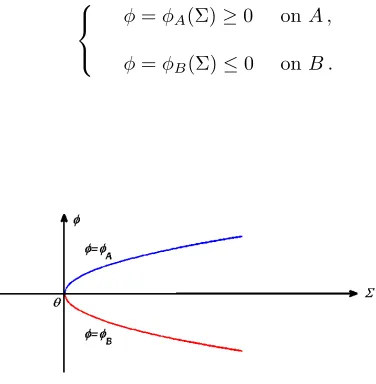
Suppose 0< z≤g. ThenφAandφBcan be regarded as one variableφandc1−c2may become

Proposition 2.1. Suppose 0< z ≤g. Then Σ = Σ(φ) can be a single-valued function of φwith domain being the entire spaceRand range[Σz,∞)such that Σ(0) = Σz,







φA(Σ(φ)) =φ ifφ≥0,

φB(Σ(φ)) =φ ifφ≤0,

(2.13)

andc1−c2= (c1−c2) (Σ (φ))is a strictly monotone increasing function ofφfrom−∞to∞.

Proof. Suppose 0< z≤g. Then by (2.11) and (2.12), we have

d

dΣφA(Σ)>0 and d

dΣφB(Σ)<0 for Σ≥Σz. (2.14) Here we have used 0< z≤g. ThusφA(Σ)>0 andφB(Σ)<0 for Σ>Σz. Besides, the range of

φA is [0,∞) and the range of φB is (−∞,0]. Note thatφA(Σz) =φB(Σz) = 0. We may combine

φAandφB as one variableφ(see Figure 1) defined as follows:







φ=φA(Σ)≥0 onA ,

φ=φB(Σ)≤0 onB .

Figure 1: θ= (Σz,0) in (Σ, φ) coordinates

Hence by (2.14) and inverse function theorem, Σ can be denoted as Σ = Σ(φ) and become a single-valued function ofφwith domain being the entire spaceRand range [Σz,∞) such that Σ(0) = Σz

and (2.13) hold true. The derivative of Σ with respect toφis

dΣ dφ =

1

dφ dΣ

=



  

  

qe

(g+z)Σ√_Σ2_−4e−(g+z)Σ

(1+gΣ)e(g+z)Σ+g2₋z2 if φ≥0,

−qe(g+z)Σ √

Σ2_−4e−(g+z)Σ

(1+gΣ)e(g+z)Σ_+g2_−z2 if φ≤0.

(2.15)

Moreover,c1−c2 = (c1−c2)(Σ(φ)) is also a function ofφ. Note that Σ(0) = Σz, Σ0(0) = 0 and

(c1−c2) (Σ (0)) = (c1−c2) (Σz) = 0. Then (2.8) and (2.15) imply

d

dφ(c1−c2) = d

dΣ(c1−c2) dΣ dφ =q

Σe(g+z)Σ_{+ 2 (g+z)}

(1 +gΣ)e(g+z)Σ_+g2_−z2 >0 forφ∈R.

Therefore,c1−c2 is strictly monotone increasing toφand we complete the proof.

Whenz=g12is increased, for example when the ion is divalent like calcium, the profiles ofφA

andφBmay lose monotonicity and become oscillatory. It is well known in experiments that calcium

has profound and complex effects on the current voltage relations of channels (cf. [2, 22]). Suppose z >p1 +g2_{>0. Thenz}2_−g2_{>1 and there exists a unique Σ}

c>0 (because (1 +gΣ)e(g+z)Σis

strictly monotone increasing to Σ>0) depending on Σz such that

Note that dφA

dΣ (Σc) =

dφB

dΣ (Σc) = 0 if Σc>Σz>0. We shall prove that Σc may be located in the

domain ofφA and φB i.e. Σc >Σz >0 ifz is sufficiently large (see Proposition 2.2). By (2.11)

and (2.12), dφA

dΣ <0 on (Σz,Σc),

dφA

dΣ >0 on (Σc,∞),

dφB

dΣ >0 on (Σz,Σc),

dφB

dΣ <0 on (Σc,∞).

Then Σc is a unique (global) minimal point of φA and a unique (global) maximal point of φB,

respectively (see Figure 2). Moreover, by (2.10),

φA,c≡ −φA(Σc) =−min

Σ>Σz

φA(Σ) = max

Σ>Σz

φB(Σ) =φB(Σc)>0. (2.16)

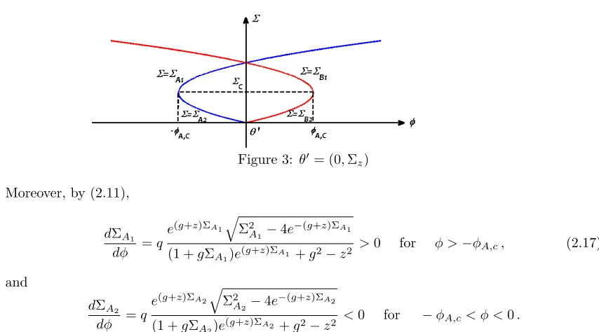
Figure 2: θ= (Σz,0) in (Σ, φ) coordinates

By Figure 2, the inverse image of functionφAconsists of two functions ΣA1: (−φA,c,∞)→(Σc,∞)

and ΣA2 : [−φA,c,0] →[Σz,Σc] such that

dΣA1

dφ >0 on (−φA,c,∞) and dΣA2

dφ <0 on (−φA,c,0)

(see Figure 3).

Figure 3: θ0 = (0,Σz)

Moreover, by (2.11),

dΣA1

dφ =q

e(g+z)ΣA1

q

Σ2

A1−4e

−(g+z)ΣA1

(1 +gΣA1)e

(g+z)ΣA1+g2−z2

>0 for φ >−φA,c, (2.17)

and

dΣA2

dφ =q

e(g+z)ΣA2

q

Σ2

A2−4e

−(g+z)ΣA2

(1 +gΣA2)e

(g+z)ΣA2+g2−z2

<0 for −φA,c< φ <0.

Similarly, the inverse image of functionφB consists of another two functions ΣB1 : (−∞, φA,c)→

(Σc,∞) and ΣB2 : [0, φA,c]→[Σz,Σc] such that

dΣB1

dφ <0 on (−∞, φA,c) and dΣB2

dφ >0 on (0, φA,c).

Moreover, by (2.12),

dΣB1

dφ =−q

e(g+z)ΣB₁ q

Σ2

B1−4e

−(g+z)ΣB₁

(1 +gΣB1)e

(g+z)ΣB1 +g2−z2

and

dΣB2

dφ =−q

e(g+z)ΣB2

q

Σ2

B2−4e

−(g+z)ΣB2

(1 +gΣB2)e

(g+z)ΣB_2+g2_−z2 >0 for 0< φ < φA,c.

Thus by (2.8), we may consider two functions of (c1−c2)◦ΣA1 and (c1−c2)◦ΣB1 as follows:

(c1−c2)(ΣA1(φ)) =

q

Σ2

A1−4e

−(g+z)ΣA1 for φ≥ −φ_A,c, (2.19)

and

(c1−c2)(ΣB1(φ)) =−

q

Σ2

B1−4e

−(g+z)ΣB1 for φ≤φ_A,c. (2.20)

Note that (c1−c2)(ΣA1(·)) and (c1−c2)(ΣB1(·)) are continuous functions on [−φA,c, φA,c].

More-over, by (2.17)-(2.20), we have

d

dφ(c1−c2)(ΣA1(φ)) =q

e(g+z)ΣA1[Σ_A

1+ 2(g+z)e

−(g+z)ΣA1]

(1 +gΣA1)e

(g+z)ΣA_{1 +g}2_−z2 >0 for φ >−φA,c, (2.21)

and

d

dφ(c1−c2)(ΣB1(φ)) =q

e(g+z)ΣB1[Σ_B

1+ 2(g+z)e

−(g+z)ΣB1]

(1 +gΣB1)e

(g+z)ΣB_{1 +g}2_−z2 >0 for φ < φA,c. (2.22)

Here we have used (2.38) and (2.39). Consequently, (c1−c2)(ΣA1(·)) and (c1−c2)(ΣB1(·)) are

smooth functions on (−φA,c, φA,c). Since (c1−c2)(ΣA1(·)) and (c1−c2)(ΣB1(·)) are strictly

mono-tone increasing toφ(see (2.21) and (2.22)), then we may use (2.8) to get

(c1−c2)(ΣA1(φ))≥(c1−c2)(ΣA1(−φA,c)) =

q

Σ2

c−4e−(g+z)Σc >0, (2.23)

(c1−c2)(ΣB1(φ))≤(c1−c2)(ΣB1(φA,c)) =−

q

Σ2

c−4e−(g+z)Σc <0, (2.24)

forφ∈(−φA,c, φA,c).

Now we claim that ifzis sufficiently large, then Σc >Σz>0 i.e. Σc is located in the domain

ofφAandφB as follows:

Proposition 2.2. Let

gc= inf{z >

p

1 +g2_{: there existsΣ}

c,z>Σz>0 such that(1 +gΣc,z)e(g+z)Σc,z+g2−z2= 0},

(2.25)

whereΣz>0 is the unique solution of Σ = 2e−

1

2(g+z)Σ forz >0. Then for z > g_c, there exists a

uniqueΣc = Σc,z>Σz depending onz such that(1 +gΣc)e(g+z)Σc+g2−z2= 0. Conversely, for

0< z < gc, no suchΣc exists and(1 +gΣ)e(g+z)Σ+g2−z2>0 forΣ≥Σz >0.

Proof. Firstly, we claim thatgcis well-defined. For anyz >0, we may define a functionfz=fz(Σ)

by

fz(Σ) = (1 +gΣ)e(g+z)Σ+g2−z2 for Σ>0. (2.26)

Then it is obvious thatfz(+∞) =∞,

f_z0(Σ) = [g+ (1 +gΣ)(g+z)]e(g+z)Σ>0 for Σ, z >0, (2.27)

and fz(0) = 1 +g2−z2 < 0 if z >

p

1 +g2_{. Hence there exists a unique Σ}

c,z > 0 such that

fz(Σc,z) = 0. Let Σ///z>0 be the unique solution of

Σz= 2e−

1

2(g+z)Σz _{for z >0. (2.28)}

Now we prove Σc,z>Σz asz sufficiently large. By (2.28), Σz is decreasing to z (differentiate

(2.28) toz) andz=−g+2 ln Σz−ln 4

Σz

. Thus Σz→0 asz→ ∞and

fz(Σz) = (1 +gΣz)e(g+z)Σz +g2−z2

= [4(1 +gΣz) + (g2−z2)Σ2z]/Σ

2

z by (2.28)

and thenfz(Σz)< 0 asz sufficiently large. Sincefz(Σc,z) = 0 andfz(Σz)< 0 asz sufficiently

large, then by (2.27), we have Σc,z>Σz asz sufficiently large. Consequently, the set

Z ={z >p1 +g2_:∃Σ

c,z>Σz>0 such thatfz(Σc,z) = 0} (2.29)

={z >p1 +g2_:f

z(Σz)<0}

is nonempty and the valuegc= inf

z∈Zz(defined in (2.25)) is well-defined. Note that the existence of

Σc,zwithfz(Σc,z) = 0 is guaranteed due toz >

p

1 +g2_{, so (2.27) implies Σ}

c,z>Σziffz(Σz)<0

holds true.

To complete the proof of Proposition 2.2, we need the following result: Claim 1.Suppose fz0(Σz0) = 0 and Σz0 >0 for some z0 >

p

1 +g2_{. Then there exist z}

l, zr >

p

1 +g2 _andz

l< z0< zr such that fz(Σz)>0 forz∈(zl, z0)andfz(Σz)<0 forz∈(z0, zr).

Proof. By (2.26) and (2.28),

f(Σz) =

4 (1 +gΣz)

Σ2

z

+g2−z2. (2.30)

Thenfz0(Σz0) = 0 gives

41 +gΣz0

Σ2

z0

=z₀2−g2,

and Σz0 satisfies (z

2

0−g2)Σ2z0−4gΣz0−4 = 0 having solutions as Σz0 =

2

z0−g and Σz0 =−

2

z0+g.

Hence due to Σz0 >0,

Σz0=

2 z0−g

. (2.31)

Note thatz0>

p

1 +g2_{>±g. Differentiating (2.28) and (2.30) toz, we have}

d

dzfz(Σz) =−4

2 +gΣz

Σ3

z

dΣz

dz −2z ,

dΣz

dz =

−Σ2

z

(g+z)Σz+ 2

.

Thus by (2.31), we obtain

d

dzfz(Σz)|z=z0 =−z0−g <0. (2.32)

Therefore, by (2.32), we may complete the proof of Claim 1.

It is obvious that

fz(Σ)>0 for Σ>0 and 0< z≤

p

1 +g2_{. (2.33)}

Now we want to prove that

Z= (gc,∞), (2.34)

wheregc= inf

z∈Zz. Due to the continuity offz, (2.29) implies that the setZis open. Suppose the set

Z has two components. Then without loss of generality, we may assume that there existsza> gc

such thatZ = (gc, za)∪(za,∞). Hence fza(Σza) = 0 and fz(Σz)<0 for z ∈ (gc, za)∪(za,∞).

However, Claim 1 implies that fz(Σz) > 0 for z ∈ (zl, za) which contradicts to fz(Σz) < 0 for

z∈(gc, za). Thus the proof of (2.34) is done. On the other hand, Claim 1 also implies that

fz(Σz)>0 for 0< z < gc. (2.35)

Otherwise, by (2.33), there existszb∈(

p

1 +g2_{, g}

c) such thatfzb(Σzb) = 0. Then as for (2.32), we

have _dzdfz(Σz)|z=zb=−zb−g <0 and hence there existszc∈(zb, gc) such thatfzc(Σzc)<0 which

Remark 2.3.

(i) The proof of Proposition 2.2 shows that fz(Σz) > 0 for 0 < z < gc and fz(Σz) < 0 for

z > gc (see (2.34) and (2.35)). Hence by the continuity of fz,fgc(Σgc) = 0.

(ii) By (2.27) and (2.35), we have

fz(Σ) = (1 +gΣ)e(g+z)Σ+g2−z2>0 for Σ≥Σz and 0< z < gc. (2.36)

(iii) By (2.26), fz(Σz)> 0 as z =

p

1 +g2 _{but f}

gc(Σgc) = 0. Hence Remark 2.3 (i) implies

gc>

p

1 +g2_.

Suppose 0 < z < gc. Then (2.36) gives fz(Σ) >0 for Σ ≥Σz. Hence by (2.11) and (2.12), dφA

dΣ > 0 and

dφB

dΣ < 0 for Σ ≥ Σz which gives φA(Σ) > φA(Σz) = 0 = φB(Σz) > φB(Σ) for

Σ>Σz. Thus as for Proposition 2.1, Σ = Σ(φ) can be a single-valued function ofφwith domain

as the entire space R and range [Σz,∞) such that Σ(0) = Σz and c1−c2 is strictly monotone

increasing toφ. Moreover, Σ→ ∞as φ→ ±∞and (c1−c2)(Σ(φ))→ ±∞as φ→ ±∞.

Supposez > gc >0. Then Proposition 2.2 gives that there exists a unique Σc∈(Σz,∞) such

that

(1 +gΣc)e(g+z)Σc+g2−z2= 0, (2.37)

which implies

(1 +gΣ)e(g+z)Σ+g2−z2>0, for Σ>Σc, (2.38)

and

(1 +gΣ)e(g+z)Σ+g2−z2<0, for Σz≤Σ<Σc, (2.39)

By (2.9) and (2.11), we have dφA

dΣ >0 for Σ>Σc;

dφA

dΣ <0 for Σz<Σ<Σc, andφAtends to +∞

as Σ goes to +∞. Hence Σc is the unique minimum point of φA. Since Σ2z = 4e−(g+z)Σz, then

φA(Σz) = 0 which implies −φA,c =φA(Σc) <0. Since Σc satisfies (1 +gΣc)e(g+z)Σc =z2−g2

i.e. Σc+ln(1+_g+g_zΣc) =

ln(z2−g2)

g+z , then Σc must tend to zero asz goes to infinity. Note thatg >0 is

a fixed constant. Consequently,−lnh1₂Σc+

p

Σ2

c−4e−(g+z)Σc

i

→+∞asz→+∞, and then

q φA,c=q φA(Σc)

=−ln

₁

2

Σc+

q

Σ2

c−4e−(g+z)Σc

+g+z 2 Σc+

g−z 2

q

Σ2

c−4e−(g+z)Σc

=−ln

₁

2

Σc+

q

Σ2

c−4e−(g+z)Σc

+g 2

Σc+

q

Σ2

c−4e−(g+z)Σc

+z 2

Σc−

q

Σ2

c−4e−(g+z)Σc

≥ −ln

₁

2

Σc+

q

Σ2

c−4e−(g+z)Σc

→+∞

as z → +∞. Thus φA,c → +∞ as z → +∞ and g > 0 is fixed. Besides, since e−(g+z)Σc =

(1 +gΣc)/(z2−g2) and Σc→0 asz→ ∞, then by (2.8), we have (c1−c2)(Σc)→0 asz→+∞

andg >0 is fixed. Therefore, we may summarize the above results as follows:

Theorem 2.4.

(i) Suppose0< z < gc. Then(c1−c2)◦Σis a monotone increasing function toφ∈Rsatisfying

(c1−c2)(Σ(φ))→ ±∞asφ→ ±∞, respectively.

(ii) Suppose z > gc. Then there are two functions ΣA1 and ΣB1 such that (c1−c2)◦ΣA1 :

[−φA,c,∞)→Rand(c1−c2)◦ΣB1 : (−∞, φA,c]→Rare monotone increasing functions of

φ, whereφA,c satisfies φA,c → +∞ and (c1−c2)(Σc)→ 0 as z →+∞ and g >0 is fixed.

Moreover,

(c1−c2)◦ΣA1(−φA,c) = (c1−c2)(Σc)>0,

(c1−c2)◦ΣB1(φA,c) =−(c1−c2)(Σc)<0,

lim

φ→∞(c1−c2)◦ΣA1(φ) =∞ and φ→−∞lim (c1−c2)◦ΣB1(φ) =−∞.

3

Proof of Theorem 1.1 and 1.2

3.1

Proof of Theorem 1.1

In this section, we study multiple solutions of the system of equations (1.9)-(1.11) withN = 3 and the following assumptions:

ρ0>0, gi3=g3i= 0 for i= 1,2,3. (3.1)

Then we may get solutions of (1.9) by solving

lnci+ziφ+

2

X

j=1

gijcj = 0 for i= 1,2, (3.2)

and let

c3=e−z3φ. (3.3)

Note that (3.2) is same as (1.9) withN = 2. Assume

z2=−z1=q≥1, g11=g22>0 and g12> gc>0, (3.4)

wheregc>0 is a sufficiently large constant defined in Proposition 2.2. We shall use (3.4) and set

ρ0>0 in order to apply Theorem 2.4 (ii) (in Section 2) and Lemma 4.1 (in Section 4) for the proof

of Theorem 1.1 which gives multiple solutions of (1.9)-(1.11) withN = 3 andρ0>0.

By Theorem 2.4 (ii), equation (3.2) has multiple solutions

(c1, c2) = (c1(ΣA1(φ)), c2(ΣA1(φ))) and (c1, c2) = (c1(ΣB1(φ)), c2(ΣB1(φ))) (3.5)

such thatfA1(φ) =q(c1−c2) (ΣA1(φ)) andfB1(φ) =q(c1−c2) (ΣB1(φ)) are monotone increasing

toφbut the values offA1andfB1are away from zero (see Figure 4). By Lemma 4.5, it is impossible

to get uniformly bounded solution by solving eitherεφ00(x) =fA1(φ(x)) orεφ

00_{(x) =f}

B1(φ(x)) for

x∈ (−1,1). This motivates us to develop Lemma 4.1 (in Section 4), and use (3.3) to transform (1.10) into the following equations:

εφ00(x) =fA(φ(x)) for x∈(−1,1), (3.6)

and

εφ00(x) =fB(φ(x)) for x∈(−1,1), (3.7)

where

fA(φ) =q(c1−c2) (ΣA1(φ))−z3e

−z3φ_+ρ

0,

and

fB(φ) =q(c1−c2) (ΣB1(φ))−z3e

−z3φ_+ρ

0.

We may denotefA and fB as follows: fA(φ) =fA1(φ)−fc3(φ) andfB(φ) =fB1(φ)−fc3(φ),

wherefA1(φ) =q(c1−c2) (ΣA1(φ)),fB1(φ) =q(c1−c2) (ΣB1(φ)), andfc3(φ) =z3e

−z3φ_−ρ

0.

Letρ0>0. Then Theorem 2.4 (ii) (in Section 2) implies that asg12=z≥gρ0 > gc>0 (gρ0 is

a large constant depending onρ0), both functions fA1 andfB1 intersect with the function fc3 at

φA1,0andφB1,0, respectively (see Figure 4). Note that the assumptionρ0>0 is necessary for the

existence ofφA1,0 andφB1,0. Moreover,fA=fA1−fc3 andfB=fB1−fc3 satisfy

(1) fA: [−φA,c,∞)→Ris smooth and strictly monotone increasing,−φA,c<0, fA(−φA,c)<

0, fA(∞)>0 andfA(φA1,0) = 0 for someφA1,0>−φA,c.

(2) fB : (−∞, φA,c] → R is smooth and strictly monotone increasing, φA,c > 0, fB(φA,c) >

0, fB(−∞)<0 andfB(φB1,0) = 0 for someφB1,0< φA,c.

Hence by Lemma 4.1, we may get uniformly bounded solutions φA

ε and φBε of (3.6) and (3.7),

respectively. Moreover,φA

ε (x)→φA1,0 andφ

B

ε (x)→φB1,0 for x∈(−1,1) asε→0. Therefore,

we complete the proof of Theorem 1.1.

3.2

Proof of Theorem 1.2

Let N = 4, z2 = −z1 = q1 ≥ 1 and z4 = −z3 = q2 ≥ 1. Assume g11 = g22 = g > 0,

g33=g44= ˜g >0 andgij =gji= 0 fori= 1,2 andj= 3,4. Then (1.9) may be represented as

lnci+ziφ+

2

X

j=1

gijcj= 0 for i= 1,2, (3.8)

and

lnci+ziφ+

4

X

j=3

gijcj= 0 for i= 3,4. (3.9)

Note that both (3.8) and (3.9) have the same form as (3.2) with (3.4) which can be solved explicitly. As for Theorem 2.4 in Section 2, both (3.8) and (3.9) have two branches of solutions, respectively. We may denote these solutions as follows:

(c1, c2) = (c1(ΣA1(φ)), c2(ΣA1(φ))),

(c1, c2) = (c1(ΣB1(φ)), c2(ΣB1(φ))),

(c3, c4) = (c3(ΣM1(φ)), c4(ΣM1(φ))) ,

(c3, c4) = (c3(ΣN1(φ)), c4(ΣN1(φ))),

such that (c1−c2)◦ΣA1 : [−φA,c,∞)→R, (c1−c2)◦ΣB1 : (−∞, φA,c] →R, (c3−c4)◦ΣN1 :

[−φM,c,∞)→Rand (c3−c4)◦ΣM1 : (−∞, φM,c] →R, are monotone increasing functions ofφ,

whereφA,c, φM,c>0 are constants, ΣA1, ΣB1, ΣM1 and ΣN1 are functions satisfying

(c1−c2)◦ΣA1(−φA,c),(c3−c4)◦ΣN1(−φM,c)>0,

(c1−c2)◦ΣB1(φA,c),(c3−c4)◦ΣM1(φM,c)<0,

lim

φ→∞(c1−c2)◦ΣA1(φ) = limφ→∞(c3−c4)◦ΣN1(φ) =∞,

lim

φ→−∞(c1−c2)◦ΣB1(φ) =φ→−∞lim (c3−c4)◦ΣM1(φ) =−∞.

Here ◦ denotes function composition. Moreover, Theorem 2.4 gives φA,c, φM,c →+∞and (c1−

c2)◦ΣA1(−φA,c),(c1−c2)◦ΣB1(φA,c),(c3−c4)◦ΣM1(φM,c) and (c3−c4)◦ΣN1(−φM,c) tend to

zero asz,z˜→+∞andg,˜g >0 are fixed.

Without loss of generality, we may assumeφM,c < φA,c. Fixρ0 ∈Rarbitrarily. Then as for

(3.2), we may solve (3.8) and get functionsfA1(φ) =q1(c1−c2) (ΣA1(φ))−ρ0andfB1(φ) =q1(c1−

c2) (ΣB1(φ))−ρ0which are sketched in Figure 5 (up to a shift byρ0), provided thatg12=g21=z >

0 is sufficiently large. Similarly, we may solve (3.9) and get functionsfM1(φ) =q2(c4−c3) (ΣM1(φ))

andfN1(φ) =q2(c4−c3) (ΣN1(φ)) as g34=g43= ˜z >0 sufficiently large (see Figure 5). Because

function q2(c3−c4)◦ΣM1 is negative and increasing to φ, function q2(c4−c3)◦ΣM1 becomes

positive and decreasing toφ. On the other hand, functionq1(c1−c2)◦ΣA1 −ρ0 is positive and

increasing to φ. This implies that as z and ˜z sufficiently large, functions q1(c1−c2)◦ΣA1−ρ0

andq2(c3−c4)◦ΣM1 may intersect at φ=φA1,0. Similarly, functionsq1(c1−c2)◦ΣB1−ρ0and

andφB1,0 can be different by choosingzand ˜z suitably e.g.z and ˜z sufficiently large.

Figure 5: Figures offA1,fB1,fM1 andfN1

LetfA=fA1−fM1 andfB =fB1−fN1. Then

fA(φ) =q1(c1−c2) (ΣA1(φ)) +q2(c3−c4) (ΣM1(φ))−ρ0,

and

fB(φ) =q1(c1−c2) (ΣB1(φ)) +q2(c3−c4) (ΣN1(φ))−ρ0,

satisfy

(1) fA: [−φA,c, φM,c]→Ris smooth and strictly monotone increasing,−φA,c<0, fA(−φA,c)<

0, fA(φM,c)>0 andfA(φA1,0) = 0 for someφA1,0>−φA,c.

(2) fB : [−φM,c, φA,c] →R is smooth and strictly monotone increasing, φA,c >0, fB(φA,c) >

0, fB(−φM,c)<0 andfB(φB1,0) = 0 for someφB1,0< φA,c.

Moreover, equation (1.10) can be expressed asεφxx =fA(φ) and εφxx =fB(φ) for x∈ (−1,1)

which have the same forms as equations (3.6) and (3.7), respectively. Therefore by Lemma 4.1, we may complete the proof of Theorem 1.2.

4

Uniformly bounded solutions

In this section, we consider the equation

εφ00(x) =f(φ(x)) for x∈(−1,1), (4.1)

with the Robin boundary condition

φ(1) +ηεφ0(1) =φ0(1) and φ(−1)−ηεφ0(−1) =φ0(−1), (4.2)

whereφ0(1), φ0(−1) are constants andηε is a non-negative constant. Note that the solutionφεof

(4.1)-(4.2) may depend on the parameterε. For notational convenience, we omitεand denoteφ as the solution of (4.1)-(4.2). To get uniform boundedness ofφ, we assume the functionf satisfies one of the following conditions:

(F1) f : [A, M] → R is smooth and strictly monotone increasing, A < 0, f(A) < 0,0 < M ≤

∞, f(M)>0 andf(φA) = 0 for someA < φA< M.

(F2) f : [−M, B]→_Ris is smooth and strictly monotone increasing,B >0, f(B)>0,0< M ≤ ∞, f(−M)<0 andf(φB) = 0 for some−M < φB < B.

Then we have

Lemma 4.1. Assume the functionf satisfies either (F1) or (F2), and the constantsA≤φ0(−1),

φ0(1) ≤ M as (F1) holds, and −M ≤ φ0(−1), φ0(1) ≤ B as (F2) holds. Let c = φA if (F1)

holds, andc=φB if (F2) holds. Letφbe a nonconstant solution of (4.1) with the Robin boundary

(i) If φ0(1), φ0(−1)> c, then there existsx1∈(−1,1) such thatφ0(x1) = 0, φ(x1)> c, andφ

is strictly monotone decreasing in(−1, x1)and increasing in (x1,1).

(ii) If φ0(1), φ0(−1)< c, then there existsx2∈(−1,1) such thatφ0(x2) = 0, φ(x2)< c, andφ

is strictly monotone increasing in(−1, x2)and decreasing in (x2,1).

(iii) Ifφ0(1)≥c≥φ0(−1), then φis monotone increasing in(−1,1).

(iv) Ifφ0(1)≤c≤φ0(−1), then φis monotone decreasing in(−1,1).

(v) min{φ0(−1), φ0(1),0} ≤φ(x)≤max{φ0(−1), φ0(1),0} forx∈(−1,1).

(vi) φ(x)→cas ε→0+, wherec=φA if (F1) holds, and c=φB if (F2) holds.

(vii) If lim

ε→0+

ε 2η2

ε

=γ >0 andφ0(±1)6=c, then the solution φhas boundary layers atx=±1.

Proof. Without loss of generality, we may assume the function f satisfying (F1). Replacingφ by φ+c, we may assumec= 0 andf(0) = 0 in the whole proof for notational convenience. Since the domain of the functionf is only [A, M], then we firstly extend it smoothly to the entire real line

Rin order to use the standard direct method to get the existence of solution φ. Hence we may

temporarily assume the function f as a smooth and strictly monotone increasing function on _R. Actually, such an assumption can be ignored because of (4.5).

To prove Lemma 4.1, we need the following Proposition:

Proposition 4.2.

(a) Ifxa ∈(−1,1) is a local minimum point of φ, then φ(xa)>0,φis monotone decreasing in

(−1, xa)and increasing in (xa,1).

(b) If xb∈(−1,1) is a local maximum point of φ, then φ(xb)<0,φ is monotone increasing in

(−1, xb)and decreasing in (xb,1).

The proof of Proposition 4.2 (b) is quite similar to that of Proposition 4.2 (a) so we only state the proof of Proposition 4.2 (a) as follows: Supposexa ∈(−1,1) is a local minimum point

of φ. Then φ0(xa) = 0 and φ00(xa) ≥ 0. If φ00(xa) = 0, then the equation εφ00 = f(φ) gives

f(φ(xa)) =εφ00(xa) = 0 which impliesφ(xa) = 0 and then by the uniqueness of ordinary differential

equations andφ(xa) =φ0(xa) = 0, we haveφ≡0 which contradicts to φis nonconstant. Hence

φ00(xa) >0 and f(φ(xa)) = εφ00(xa) >0 i.e. φ(xa) >0. Now we prove that φ is decreasing in

(−1, xa) and increasing in (xa,1). Suppose not. Then there existsxc∈(−1,1) andxc 6=xa such

that xc is a local maximum point of φ i.e. φ0(xc) = 0, φ00(xc) ≤ 0 and φ(xc) > φ(x1) > 0 but

εφ00(xc) =f(φ(xc))>0 which contradicts to φ00(xc)≤0. Therefore, we may complete the proof

of Proposition 4.2.

For the proof Lemma 4.1 (i), we need

Claim 1.Assume φ0(1), φ0(−1)>0. Then φ(−1), φ(1)>0,φ0(−1)<0 andφ0(1)>0.

We may prove Claim 1 by contradiction. Suppose one of the following cases holds: Case I.φ(−1)>0 andφ0(−1)≥0.

Case II.φ(−1)≤0.

For the Case I, we may use φ(−1) >0 and the continuity ofφ to obtain that asx∈ (−1,1) sufficiently close to −1, φ(x) > 0 and εφ00(x) = f(φ(x)) > 0 which implies lim

x→−1+εφ

00_{(x) =}

f(φ(−1))>0. Sinceφ0(−1)≥0 and lim

x→−1+φ

00_{(x)>0, thenφis monotone increasing in (−1,−1 +}

δ0), where δ0 > 0 is a constant. Now we may show that φ is monotone increasing in (−1,1)

by contradiction. Suppose φ has a local maximum point at x0 ∈ (−1,1) such that φ0(x0) = 0,

φ00(x0)≤0 andφis monotone increasing in (−1, x0). However,εφ00(x0) =f(φ(x0))≥f(φ(−1))>

0 contradicts toφ00(x0)≤0. Hence φ is monotone increasing in (−1,1) which provides φ00(x) = 1

εf(φ(x)) ≥

1

εf(φ(−1)) i.e. φ

00_{(x) ≥} 1

εf(φ(−1)) for x∈ (−1,1). Integrating the inequality from

−1 to x, we have φ0(x)−φ0(−1)≥ 1

εf(φ(−1))(x+ 1) i.e.φ

0_(x)≥φ0_{(−1) +} 1

εf(φ(−1))(x+ 1) for

x∈(−1,1) which implies

φ(1)−φ(−1) =

Z 1

−1

φ0(x)dx≥

Z 1

−1

φ0(−1) + 1

εf(φ(−1))(x+ 1)

dx= 2

φ0(−1) +1

εf(φ(−1))

i.e.φ(1)≥φ(−1) + 2

φ0(−1) +1

εf(φ(−1))

≥ 2

εf(φ(−1)). On the other hand, the Robin boundary

condition (4.2) givesφ0(1) =φ(1) +ηεφ0(1)≥φ(1) andφ(−1) =φ0(−1) +ηεφ0(−1)≥φ0(−1)>0

sinceφis monotone increasing in (−1,1). Thus

φ0(1)≥φ(1)≥

2

εf(φ(−1))≥ 2

εf(φ0(−1)),

which contradicts to the hypothesis thatφ0(1), φ0(−1) are independent toε.

For the Case II, we first use the Robin boundary condition (4.2) to get ηεφ0(−1) = φ(−1)−

φ0(−1)≤ −φ0(−1)<0 which impliesηε>0 andφ0(−1)<0. Thenφ(x)<0 forx∈(−1,−1 +δ1)

andφ is monotone decreasing in (−1,−1 +δ1), where δ1>0 is a constant. Hence φ is negative

and monotone decreasing in (−1,1). Otherwise, there existsx3∈(−1,1) a local minimum point

of φ such that φ(x3) < 0 and φ00(x3) ≥ 0 but φ00(x3) = 1_εf(φ(x3)) < 0 which contradicts to

φ00(x3) ≥0. Such a contradiction shows thatφ is negative and monotone decreasing in (−1,1).

However, 0> φ(1) =φ0(1)−ηεφ0(1)≥φ0(1) contradicts to φ0(1)>0. Notice that both Case I

and II produce contradiction. Similarly, the condition φ(1) > 0 and φ0(1) ≤ 0 and the other conditionφ(1)≤0 also result in contradiction, respectively. Therefore, we may complete the proof of Claim I.

By Claim I, there exists x1 ∈ (−1,1) a local minimum point of φ, and then by

Proposi-tion 4.2 (a), we may complete the proof of Lemma 4.1 (i). On the other hand, we may also use the similar argument of Claim I to prove that there existsx2∈(−1,1) a local maximum point of

φ. Hence by Proposition 4.2 (b), we complete the proof of Lemma 4.1 (ii).

Now we prove Lemma 4.1 (iii) by contradiction. Suppose φ is not monotone increasing. By Proposition 4.2, it is sufficient to consider two cases as follows: φ(−1) < 0 and φ(−1) > 0. If φ(−1) < 0, then Proposition 4.2 implies that there exists x2 ∈ (−1,1) a maximum point of φ

such thatφ(x2)<0,φis monotone increasing in (−1, x2) and decreasing in (x2,1) soφ0(1)≤0.

However, the boundary condition φ(1) +ηεφ0(1) = φ0(1) and φ0(1) ≤ 0 give φ0(1) ≤ φ0(1)−

ηεφ0(1) =φ(1)≤φ(x2)<0 which contradicts toφ0(1)≥c= 0. On the other hand, ifφ(−1)>0,

then Proposition 4.2 implies that there exists x1 ∈ (−1,1) a minimum point of φ such that

φ(x1)>0,φis monotone decreasing in (−1, x1) and increasing in (x1,1) soφ0(−1)≤0. However,

the boundary condition φ(−1)−ηεφ0(−1) = φ0(−1) and φ0(−1) ≤ 0 give φ0(−1) = φ(−1)−

ηεφ0(−1)≥φ(−1)>0 which contradicts toφ0(−1)≤c= 0. Therefore, we complete the proof of

Lemma 4.1 (iii). Similar argument of Lemma 4.1 (iii) can be applied to prove Lemma 4.1 (iv) and we omit the detail here.

Using Lemma 4.1 (i)-(iv), we may prove min{φ0(−1), φ0(1),0} ≤φ(x)≤max{φ0(−1), φ0(1),0}

forx∈(−1,1). The proof is stated as follows: By Lemma 4.1 (i) and the boundary condition (4.2), we haveφ(−1) =φ0(−1)+ηεφ0(−1)≤φ0(−1),φ(1) =φ0(1)−ηεφ0(1)≤φ0(1) andc= 0< φ(x1)≤

φ(x)≤max{φ(1), φ(−1)} ≤max{φ0(1), φ0(−1)}forx∈(−1,1). Similarly, Lemma 4.1 (ii) and the

boundary condition (4.2) implyφ(−1) =φ0(−1) +ηεφ0(−1)≥φ0(−1), φ(1) =φ0(1)−ηεφ0(1)≥

φ0(1) and c = 0> φ(x2)≥φ(x) ≥min{φ(1), φ(−1)} ≥ min{φ0(1), φ0(−1)} for x∈ (−1,1). On

the other hand, we may apply Lemma 4.1 (iii) and the boundary condition (4.2) to getφ(−1) = φ0(−1) +ηεφ0(−1) ≥ φ0(−1), φ(1) = φ0(1)−ηεφ0(1) ≤ φ0(1) and φ0(−1) ≤ φ(−1) ≤ φ(x) ≤

φ(1) ≤φ0(1) for x ∈ (−1,1). Similarly, Lemma 4.1 (iv) and the boundary condition (4.2) give

φ(−1) =φ0(−1) +ηεφ0(−1) ≤φ0(−1), φ(1) = φ0(1)−ηεφ0(1) ≥φ0(1) and φ0(−1) ≥φ(−1) ≥

φ(x)≥φ(1)≥φ0(1) forx∈(−1,1). Hence we complete the proof of Lemma 4.1 (v) i.e.

min{φ0(−1), φ0(1),0} ≤φ(x)≤max{φ0(−1), φ0(1),0} for x∈(−1,1). (4.3)

LetA0= min{φ0(−1), φ0(1),0} andA1= max{φ0(−1), φ0(1),0}. Then (4.3) implies

kφkL∞ ≤A₂= max{−A₀, A₁}. (4.4)

SinceA≤φ0(−1), φ0(1)≤M and A <0, then (4.3) gives

φ(x)∈[A0, A1]⊂[A, M] for x∈(−1,1), (4.5)

Now we claim thatφ(x)→0 asε→0+ forx∈(−1,1). To prove this, we remark that

ε 2(φ

2₎00_{(x) =ε(φφ}00_{+ (φ}0₎2_{)(x)≥εφφ}00_{(x) =φ(x)f(φ(x)) =φ(x)}Z

φ(x)

0

f0(s)ds≥α0φ2(x),

forx∈(−1,1), whereα0= minz∈[A0,A1]f

0_{(z)>0 is a constant coming from the strictly monotone}

increasing off. Note that ifφ(x)<0, then

φ(x)

Z φ(x)

0

f0(s)ds= (−φ(x))

Z 0

φ(x)

f0(s)ds≥(−φ(x))

Z 0

φ(x)

α0ds=α0φ2(x).

Since ε

2(φ

2₎00_(x)≥α

0φ2(x) forx∈(−1,1), then by (4.4) and the standard comparison theorem,

we have φ2_{(x) ≤ A}2 2

e−(1+x)√2α0/ε_+e−(1−x)

√

2α0/ε _{for x ∈ (−1,1). Therefore, φ(x) → 0 as}

ε→0+ forx∈(−1,1), and we may complete the proof of Lemma 4.1 (vi).

For the proof of Lemma 4.1 (vii), we firstly multiply the equation (4.1) byφ0. Then we have

ε

2

(φ0)20=εφ0φ00=f(φ)φ0=_dxdF(φ), which implies ε

2(φ

0_(x))2

=F(φ(x)) +Cε, (4.6)

for x∈ (−1,1), where F(φ) =

Z φ

0

f(s)ds and Cε is a constant depending on ε. Now we want

to claim that lim

ε→0+Cε = 0. By the mean value theorem, there exists xε ∈ (− 1 2,

1

2) such that

φ(1₂)−φ(−1 2) = φ

0_(x

ε). Since φ(x)→ 0 asε →0+ for x∈ (−1,1), thenφ(1₂), φ(−1₂)→ 0 and

φ0_(x

ε) =φ(1₂)−φ(−1₂)→0 asε→0+. Hence by (4.6), we obtainCε= ε₂(φ0(xε))2−F(φ(xε))→0

asε→0+ i.e. lim

ε→0+Cε= 0. On the other hand, we may put the Robin boundary condition (4.2)

into (4.6) and get₂ε_η2

ε(φ0(1)−φ(1))

2

=F(φ(1))+Cεand_2ηε2

ε(φ0(−1)−φ(−1))

2

=F(φ(−1))+Cε.

By (4.5) and the continuity ofφ, we may assumeφ(±1)→φ∗(±1) asε→0+ (up to a subsequence).

Generically, the valuesφ∗(1) andφ∗(−1) may not be uniquely determined but here we want to claim

the uniqueness ofφ∗(±1) as follows: Suppose lim

ε→0+

ε 2η2

ε

=γ >0. Thenφ∗(1) andφ∗(−1) satisfy

√

γ|φ0(1)−φ∗(1)|= p

F(φ∗(1)) and

√

γ|φ0(−1)−φ∗(−1)|= p

F(φ∗(−1)). Notice that the function

Fis positive and monotone increasing in (0, M] and decreasing in [A,0) becauseF0(φ) =f(φ)>0 on (0, M) and<0 on (A,0). Here we have used the fact thatφA=c= 0. By Lemma 4.1 (i)-(iv),

we have√γ|φ0(±1)−φ∗(±1)| =

√

γ(φ0(±1)−φ∗(±1)) if φ0(±1) > 0;

√

γ|φ0(±1)−φ∗(±1)| =

√

γ(φ∗(±1)−φ0(±1)) ifφ0(±1)<0;

√

γ|φ0(±1)−φ∗(±1)|=±

√

γ(φ0(±1)−φ∗(±1)) ifφ0(−1)≤

0 ≤φ0(1); and

√

γ|φ0(±1)−φ∗(±1)| =±

√

γ(φ∗(±1)−φ0(±1)) if φ0(−1) ≥0 ≥φ0(1). Hence

φ∗(±1) can be uniquely determined by the equations

√

γ|φ0(1)−s|=

p

F(s) and√γ|φ0(−1)−s|=

p

F(s), respectively. The uniqueness of φ∗(±1) implies that the asymptotic limits of boundary

valuesφ(±1) are lim

ε→0+φ(±1) =φ∗(±1). One may also remark that φ∗(±1)6= 0 =c(Otherwise, if

φ∗(±1) = 0,then

√

γ|φ0(1)−φ∗(1)|= p

F(φ∗(1)),

√

γ|φ0(−1)−φ∗(−1)|= p

F(φ∗(−1)) andF(0) =

0 imply thatφ0(±1) = 0 =cwhich contradicts to the assumptionφ0(±1)6=c.) Consequently, the

solutionφhas boundary layers at x=±1 if γ >0. Therefore, we have showed Lemma 4.1 (vii) and completed the proof of Lemma 4.1.

Remark 4.3. The equation (4.1) with the boundary condition (4.2) has a unique solution.

The uniqueness comes from the strictly monotone increasing of the function f. The proof is sketched as follows: Suppose φ1 and φ2 are solutions of (4.1) and (4.2). We may subtract the

equation ofφ1by that of φ2, and multiply the resulting equation byu=φ1−φ2and integrate it

over (−1,1). Then using integration by part, we haveu0(1)u(1)−u0(−1)u(−1)−R1 −1(u

0_(x))2_dx=

R1 −1 c(x)u

2_{dx, where c(x) =} f(φ1(x))−f(φ2(x))

φ1(x)−φ2(x) is positive since the functionf is strictly monotone

increasing. On the other hand, the Robin boundary condition (4.2) gives u(−1) = ηεu0(−1),

u(1) =−ηεu0(1) andu0(1)u(1)−u0(−1)u(−1) =−ηε

(u0(−1))2_{+ (u}0₍₁₎₎2

. Hence

0≤

Z 1

−1

c(x)u2dx=−ηε(u0(−1))2+ (u0(1))2−

Z 1

−1

which impliesu≡0 i.e. φ1≡φ2 and the uniqueness proof ofφis complete.

Remark 4.4. The solution φ of the equation (4.1) with the boundary condition (4.2) has linear stability.

To get the linear stability of the solution φ of the equation (4.1) with the boundary condi-tion (4.2), we study the eigenvalue problem Lv = λv of the corresponding linearized operator Lv=−εv00_+f0_{(φ)vwith the boundary conditionv(±1)±η}

εv(±1) = 0. Using integration by part,

it is obvious that

λ

Z 1

−1

v2dx=

Z 1

−1

v Lv dx=

Z 1

−1

εv00v dx+

Z 1

−1

f0(φ)v2dx

=ηε

(v0(−1))2_{+ (v}0₍₁₎₎2

+

Z 1

−1

ε(v0)2+f0(φ)v2 dx≥µ0

Z 1

−1

v2dx , (4.7)

and henceλ≥µ0>0, where µ0 = mins∈[minφ,maxφ]f0(s) is a positive constant arising from the

strictly monotone increasing of the functionf.

In Lemma 4.1, the existence of zero point φA (or φB) off is essential. If the functionf has

not any zero point likeφA (or φB) i.e. the value off is away from zero, then the equation (4.1)

may not have uniformly bounded solutions{φ}ε>0. Such a result is stated as follows:

Lemma 4.5. Assume f is a function satisfying one of the following conditions:

(a) f : [A,∞)→Ris monotone increasing,A <0 andf(A)>0.

(b) f : (−∞, B]→Ris monotone increasing, B >0andf(B)<0.

For eachε >0, letφ be a solution of the equation (4.1). Thensup

ε>0

kφkL∞ =∞.

Proof. Without loss of generality, we may assume the functionf satisfies the condition (a). Now we prove Lemma 4.5 by contradiction. Suppose{φ}ε>0is uniformly bounded i.e. sup

ε>0

kφkL∞ <∞.

We divide three cases to complete the proof as follows:

Case I.The solutionφ=φ(x) is monotone decreasing to xi.e.φ0(x)≤0 forx∈(−1,1). Using the equationεφ00=f(φ) and the condition (a), we have

−φ0(x)≥φ0(1)−φ0(x) =

Z 1

x

φ00(τ)dτ

=ε−1

Z 1

x

f(φ(τ))dτ

≥ε−1

Z 1

x

f(A)dτ =ε−1f(A)(1−x), ∀x∈(−1,1),

and hence

−2kφkL∞≤φ(1)−φ(−1) = Z 1

−1

φ0(x)dx≤ −ε−1_f(A)

Z 1

−1

(1−x)dx=−2ε−1_f(A),

i.e.kφkL∞ ≥ε−1f(A)→ ∞as ε→0+ which contradicts to the hypothesis sup

ε>0

kφkL∞ <∞.

Case II.The solutionφ=φ(x) is monotone increasing toxi.e.φ0(x)≥0 forx∈(−1,1). As for the argument of Case I, we obtain

φ0(x)≥φ0(x)−φ0(−1) =

Z x

−1

φ00(τ)dτ

=ε−1

Z x

−1

f(φ(τ))dτ

≥ε−1

Z x

−1

and hence

2kφkL∞ ≥φ(1)−φ(−1) = Z 1

−1

φ0(x)dx≥ε−1f(A)

Z 1

−1

(1 +x)dx= 2ε−1f(A),

i.e.kφkL∞ ≥ε−1f(A)→ ∞as ε→0+ which contradicts to the hypothesis sup

ε>0

kφkL∞ <∞.

Case III.The solutionφ=φ(x) has a local minimum point atx0∈(−1,1) such that φ0(x0) = 0

andφ00(x0)>0.

Note that sinceεφ00 =f(φ)≥f(A)>0, it is impossible to have any local maximum point in (−1,1). By the equationεφ00=f(φ) and the condition (a), we have

−φ0(x) =φ0(x0)−φ0(x) =

Z x0

x

φ00(τ)dτ

=ε−1

Z x0

x

f(φ(τ))dτ

≥ε−1

Z x0

x

f(A)dτ =ε−1f(A)(x0−x), ∀x∈(−1, x0),

and hence

−2kφkL∞ ≤φ(x₀)−φ(−1) = Z x0

−1

φ0(x)dx≤ −ε−1_f(A)

Z x0

−1

(x0−x)dx=−

1 2ε

−1_f(A)(x

0+ 1)2,

i.e.

|x0+ 1| ≤2ε1/2

p

kφkL∞/f(A). (4.8)

On the other hand,

φ0(x) =φ0(x)−φ0(x0) =

Z x

x0

φ00(τ)dτ

=ε−1

Z x

x0

f(φ(τ))dτ

≥ε−1

Z x

x0

f(A)dτ =ε−1f(A)(x−x0), ∀x∈(x0,1),

and hence

2kφkL∞≥φ(1)−φ(x₀) = Z 1

x0

φ0(x)dx≥ε−1f(A)

Z 1

x0

(x−x0)dx=

1 2ε

−1_f(A)(x

0−1)2,

i.e.

|x0−1| ≤2ε1/2

p

kφkL∞/f(A). (4.9)

Therefore, asε >0 sufficiently small, (4.8) and (4.9) provide a contradiction and we may complete the proof of Lemma 4.5.

5

Excess currents due to steric effects

Here we want to use solutions φA

ε and φBε of (1.9)-(1.11) (see Theorem 1.1 and 1.2) to calculate

excess currents (due to steric effects) represented by formula (1.5). By (1.6),

N

X

j=1

gijcj =−kBTlnci−zieφ ,

and then formula (1.5) becomes

Iex=

N

X

i=1

zieDi

∇ci+zici∇φ˜

, (5.1)

where ˜φ=_ke

5.1

Under the same hypotheses of Theorem 1.1

Here we set N = 3, z2 =−z1=q ≥1, z3 >0, ρ0 >0, and assume that g11 =g22 =g >0 is

fixed, g12 =g21 =z > 0 is sufficiently large, andgi3 =g3i = 0 fori = 1,2,3. By (3.3), we have

c3=e−z3 ˜

φ_{which implies ∇c}

3+z3c3∇φ˜= 0. Hence (5.1) becomes

Iex =

2

X

i=1

zieDi

dci

dx +zici dφ˜ dx

!

= −q eD1

dc1

dx −q c1 dφ˜ dx

!

+q eD2

dc2

dx +q c2 dφ˜ dx

!

= q e

"

d

dx(−D1c1+D2c2) +q(D1c1+D2c2) dφ˜ dx

#

i.e.

Iex=q e

"

d

dx(−D1c1+D2c2) +q(D1c1+D2c2) dφ˜ dx

#

(5.2)

Usingc1= c1−₂c2 +c1+₂c2 andc2=c1+₂c2 −c1−₂c2, formula (5.2) can be expressed as 1

q eI

ex ₌ d dx

D2−D1

2 (c1+c2)−

D1+D2

2 (c1−c2)

+qD1+D2

2 (c1+c2)−

D2−D1

2 (c1−c2)

dφ˜

dx

(5.3)

Note thatc1+c2 = Σ and c1−c2 =

√

Σ2_−4e−(g+z)Σ _{on A,}

−√Σ2_−4e−(g+z)Σ _onB. (see (2.8) in Section 2).

As for (3.5)-(3.7), we may set Σ,φ˜ = ΣA1

˜ φ, φA

ε (x)

and Σ,φ˜ = ΣB1

˜ φ, φB

ε (x)

,

respectively. Then along c1+c2 = Σ = ΣA1 and c1−c2 =

q

Σ2

A1−4e

−(g+z)ΣA1, we may use

(2.17), (2.21) and Chain Rule to get

d

dx(c1+c2) = d dxΣA1 φ

A ε (x)

= dΣA1

dφ φ A ε (x) dφA ε dx (x) = r Σ2

A1(φ

A ε(x))−4e

−(g+z)Σ_A

1(φAε(x))

1+gΣA1(φAε(x))+(g2−z2)e

−(g+z)ΣA1(φAε(x))

dφA ε

dx (x),

and

d

dx(c1−c2) = d

dx(c1−c2) ΣA1 φ

A ε (x)

= d

dφ(c1−c2) ΣA1 φ

A ε (x)

dφA_ε dx (x)

= ΣA1(φ

A

ε(x))+2(g+z)e −(g+z)Σ_A

1(φAε(x))

1+gΣA1(φAε(x))+(g2−z2)e

−(g+z)ΣA₁(φA_ε(x))

dφA_ε dx (x).

For simplicity, we may set ˆΣA1 = ΣA1 φ

A ε (x)

and denote _dxd (c1±c2) as follows:

d

dx(c1+c2) =

q

ˆ Σ2

A1−4e

−(g+z) ˆΣA1

1 +gΣˆA1+ (g

2_−z2_)e−(g+z) ˆΣA₁

dφA ε

dx (x),

and

d

dx(c1−c2) = ˆ

ΣA1+ 2(g+z)e

−(g+z) ˆΣA1

1 +gΣˆA1+ (g

2_−z2_)e−(g+z) ˆΣA1

dφAε

dx (x).

Consequently, by settingIex

A =Iex alongA1, (5.3) becomes

1

q eI ex A =

D2−D1 2

r ˆ Σ2

A1−4e

−(g+z) ˆΣ_A

1−D1 +D2

2

h ˆ

ΣA1+2(g+z)e

−(g+z) ˆΣ_A 1

i

1+gΣˆA1+(g2−z2)e

−(g+z) ˆΣ_A 1

dφA_ε dx (x)

+q

D1+D2

2 ΣˆA1−

D2−D1

2

q

ˆ Σ2

A1−4e

−(g+z) ˆΣA1

dφA ε

dx (x)

Similarly, alongc1+c2= Σ = ΣB1

˜

φ,c1−c2=−

q

Σ2

B1−4e

−(g+z)ΣB1 and ˜φ=φB_ε (x), we may

setIex=I_Bex, and use (2.18) and (2.22) to get

1

q eI ex B =

D1−D2 2

r ˆ Σ2

B1−4e

−(g+z) ˆΣB1−D1 +D2 2

h ˆ

ΣB1+2(g+z)e

−(g+z) ˆΣB1i

1+gΣˆB1+(g2−z2)e

−(g+z) ˆΣB₁

dφB_ε dx (x)

+q

D1+D2

2 ΣˆB1−

D1−D2

2

q

ˆ Σ2

B1−4e

−(g+z) ˆΣB1

dφB ε

dx (x)

(5.5)

where ˆΣB1= ΣB1 φ

B ε (x)

.

Equation (5.4) and (5.5) can be denoted as

I_Aex =q e iA

ˆ ΣA1

dφA_ε

dx (x), (5.6)

and

IBex=q e iB

ˆ ΣB1

dφB_ε

dx (x), (5.7)

where

iA(Σ) =

D2−D1 2

√

Σ2_−4e−(g+z)Σ₋D1 +D2

2 [Σ+2(g+z)e

−(g+z)Σ_]

1+gΣ+(g2_−z2_)e−(g+z)Σ ,

+qhD1+D2

2 Σ−

D2−D1

2

√

Σ2_−4e−(g+z)Σi

(5.8)

and

iB(Σ) =

D1−D2 2

√

Σ2_−4e−(g+z)Σ₋D1 +D2

2 [Σ+2(g+z)e

−(g+z)Σ_]

1+gΣ+(g2_−z2_)e−(g+z)Σ .

+qhD1+D2

2 Σ−

D1−D2

2

√

Σ2_−4e−(g+z)Σi

(5.9)

Without loss of generality, φA_ε can be assumed as a monotone increasing function. Such an as-sumption can be fulfilled by setting φ0(−1) < φ0(1) and using Lemma 4.1 (iii). IntegratingIAex

fromx1 tox2, we have

Z x2

x1

I_Aexdx=e

Z x2

x1

iA ΣA1 φ

A ε (x)

dφ

A ε

dx dx=e

Z φA2

φA

1

iA(ΣA1(φ))dφ , (5.10)

for−1 < x1 < x2 <1, where φ1 ≤φ2 and φAj =φAε (xj), j = 1,2. Setting Σ = ΣA1 and using

change of variables, Inverse Function Theorem and (2.17), we have

dφ= dφ dΣdΣ =

1

dΣ

dφ

dΣ = 1 +gΣ + g

2_−z2

e−(g+z)Σ

√

Σ2_−4e−(g+z)Σ dΣ.

Then by (5.8), we get

iA(Σ)dφ=iA(Σ)

1 +gΣ + g2_−z2

e−(g+z)Σ

√

Σ2_−4e−(g+z)Σ dΣ

=D2−D1 2

n

(1−q)−qhgΣ + g2−z2e−(g+z)ΣiodΣ

− D1+D2 2√Σ2_−4e−(g+z)Σ

h

(1−q)Σ + 2 (g+z)e−(g+z)Σ−q gΣ2−q g2−z2