Active feedback acoustic noise control

INTERNSHIP REPORT

FACULTY OF ENGINEERING TECHNOLOGY

ACTIVE FEEDBACK

ACOUSTIC NOISE

CONTROL

L.R. Kamphuis

S1012428

Supervised by:

Prof.dr.ir. R.A. de Callafon

Dr.ir. R.G.K.M. Aarts

2

CONTEXT

3

ABSTRACT

Active noise control is applied at an air conditioning (AC) air duct with incoming unknown noise from an input speaker, output microphone and a feedback controller. Positioning the speaker downstream to the microphone, according to the flow direction of the incoming sound, a feedback loop can be created. Sound delay will be an issue as introduced by sound traveling over a certain distance in time. In practice, high frequency sounds will be reduced passively by a damper part in the air duct, remaining lower frequencies will be important for the active noise control loop. After identifying the sound paths in the air duct, low order stable feedback controllers can be formed using loop shaping or 𝐻2 control

4

TABLE OF CONTENTS

CONTEXT ... 2

ABSTRACT ... 3

TABLE OF CONTENTS ... 4

INTRODUCTION ... 6

I SET UP ... 7

Set up 2 ... 9

Stability ... 10

Ideal situation ... 10

II MEASUREMENTS ... 12

Cut of frequency ... 12

Acoustic paths 𝐻1 and 𝐻2 ... 12

Acoustic paths 𝐺1 and 𝐺2 ... 14

Measurement 𝐹1 and 𝐹2 ... 15

III NOMINAL MODELS ... 16

IV PRACTICE ... 18

Filters ... 19

Sample frequency ... 19

Computer ... 19

Nominal set up ... 20

V LOOP SHAPED CONTROLLER ... 21

Practice ... 23

Simulation ... 24

VI 𝐻2 CONTROLLER ... 26

Implementation ... 27

Calculate 𝐶𝐻 ... 29

VII YOULA CONTROLLER SET UP 2 ... 32

5

Trivial choice ... 33

Representation in Set up 2 ... 33

Linear in Q ... 34

FIR model ... 35

Updating ... 36

Filter W... 37

Simulation ... 38

Updating simulation ... 40

VIII YOULA CONTROLLER GENERAL SET UP ... 43

Youla parameterization General Set up ... 43

Representation General Set up ... 43

Linear in Q for General Set up ... 44

Updating ... 45

Simulation ... 45

Updating simulation ... 47

IX SIMULINK MODEL ... 49

Simulink representation... 49

Loop shaped controller ... 49

Youla Updating controller ... 50

Practice ... 50

X CONCLUSIONS ... 51

XI RECOMMANDATIONS ... 52

LITERATURE ... 54

Lecture Notes ... 54

Books and papers ... 54

APPENDIX ... 55

A. Self-made Butterworth filter ... 55

B. Proof for (VII-29) ... 57

C. SIMULINK ... 58

6

INTRODUCTION

In this report an AC air duct is used for active sound control. Inside the air duct a microphone and control speaker are positioned in such a way that a closed loop system between microphone and speaker can be created. Using static controllers (loop shaped or 𝐻2) and real-time updating controllers

the incoming sound will be measured and reduced as much as possible. The main question in this report will be: “Is it possible to reduce incoming sound using an active control feedback loop?”

Previous research with the same AC air duct is done using a feedforward static 𝐻2 controller in [19].

Obtaining a 𝐻2 controller for a standard control problem is show in [8], [4] and [7]. The updating FIR

filter used in the real time Updating Youla controller is also applied on different systems with similar properties in [11], [12], [14] and [18] in which the updating algorithm is explained in [13] and [16]. To obtain overall stability in the updating algorithm a Youla parameterization is used as explained in [15] with more details about coprime factorization in [2] and [3]. Other approaches for active noise control in an air duct are shown in [17] and [6].

Following the chapters in this report will show the same sequence as the research has taken place in practice. Starting with explaining the set up and AC air duct configuration in chapter I with measuring and analyzing all the acoustic sound paths in chapter II. Identifying the sound paths in chapter III to create nominal models for computer simulations and control purposes. In chapter IV the nominal models are used to simulate the set up in practice including filters and ADC-DAC conversion. Continuing in chapter V with applying a loop shaped controller and in chapter VI an 𝐻2 controller will be applied

7

I

SET UP

In this chapter the AC air duct in practice will be shown and discussed in detail. Schematic models corresponding to the sound paths in practice will be created. These models will be used to design a stable feedback loop of the system further on. A CAD model1 _{of the air duct is shown in Figure 1}

Figure 1: Section views of air conditioning air duct

A schematic representation of the air duct is presented in Figure 2, with the dimensions summarized in Table 1. One end (right) of the air duct is closed and the other end (left) is open. The main part of the air duct consists of foam to create a high frequency passive damper. This damping section has a length of 𝑙𝑑 and an inner diameter of 𝑑𝑖, the approximated total length of the air duct is given by 𝑙.

Figure 2: Schematic view air conditioning air duct

8 Two speakers and two microphones are positioned at certain positions inside the air duct. The first speaker, the so called ‘Ground speaker’, is positioned at the closed right end of the duct and produces an input 𝑛(𝑡). A second speaker ‘Control speaker’ is positioned in the middle of the duct at a distance

𝑙_𝑐 to the open end and represents input 𝑢(𝑡). Both microphones are placed downstream of the control speaker with a distance 𝑙1 and 𝑙2. The output of the microphones are 𝑒1(𝑡) and 𝑒2(𝑡), respectively.

Description Symbol Value

Inner diameter 𝑑𝑖 0.2 𝑚

Length of air duct 𝑙 2.4 𝑚 Length of damper 𝑙𝑑 1.4 𝑚

Position microphone 1 𝑙1 0.25 𝑚

Position microphone 2 𝑙2 0.05 𝑚

Position Control speaker 𝑙𝑐 0.30 𝑚 Table 1: Properties air duct

The whole set up contains two inputs 𝑛(𝑡) and 𝑢(𝑡) and two outputs 𝑒1(𝑡) and 𝑒2(𝑡) so in total four

acoustic paths can be composed.

𝑒₁(𝑡)

𝑛(𝑡) = 𝐻1

(I-1)

𝑒₂(𝑡)

𝑛(𝑡) = 𝐻2

(I-2)

𝑒1(𝑡)

𝑢(𝑡) = 𝐺1

(I-3)

𝑒2(𝑡)

𝑢(𝑡) = 𝐺2

(I-4)

A schematic overview of these acoustic paths is given in Figure 3.

9 Both microphone outputs can be written in terms of the speaker inputs 𝑢(𝑡) and 𝑛(𝑡) according to.

𝑒1(𝑡) = 𝐺1𝑢(𝑡) + 𝐻1𝑛(𝑡)

(I-5)

𝑒₂(𝑡) = 𝐺₂𝑢(𝑡) + 𝐻₂𝑛(𝑡)

_(I-6)

In which 𝑛(𝑡) is the input of the air duct at the ground speaker and assumed to be unknown. The other input 𝑢(𝑡) is a customizable input and can be used to create a control system. For example, create a close loop between 𝑒2(𝑡) and 𝑢(𝑡), will be named: Set up 2, or between 𝑒1(𝑡) and 𝑢(𝑡), labeled as Set

up 1. Both closed loop configuration are shown in Figure 4 and Figure 5 with unknown controller 𝐶. Based on the stability criteria explained in the next paragraph, the controller will be applied according to the Set up 2 configuration, see Figure 5. Remark: the closed loop equations for set up 1 and Set up 2 are identical for output 𝑒1(𝑡) and 𝑒2(𝑡) respectively.

Figure 4: Set up 1 Figure 5: Set up 2

S

2

The input 𝑢(𝑡) of Set up 2 can be written as.

𝑢(𝑡) = 𝐶𝑒₂(𝑡)

_(I-7)

Substitute (I-7) into (I-5) and (I-6).

𝑒₁(𝑡) = 𝐺₁𝐶𝑒₂(𝑡) + 𝐻₁𝑛(𝑡)

_(I-8)

10 Rewrite (I-9) to obtain the transfer function from the ground speaker to microphone 2.

𝑒₂(𝑡) = 𝐻2

1 − 𝐺2𝐶𝑛(𝑡)

(I-10)

In which the sensitivity function 𝑆 and closed loop gain 𝐿 are given by.

𝑆 = 1

1 − 𝐺2𝐶

(I-11)

(I-12)

Substitute (I-10) into (I-8) to obtain the transfer function from the ground speaker to microphone 1.

𝑒₁(𝑡) = (𝐻1+ 𝐻2

𝐺1𝐶

1 − 𝐺₂𝐶) 𝑛(𝑡)

(I-13)

S

To obtain a stable feedback system the controller 𝐶 must stabilize the sensitivity function 𝑆 in

(I-11)

(I-11)

only if, the following three rules are satisfied.

I. The closed loop gain 𝐿 must be stable.

II. The magnitude of the closed loop gain must be smaller than unity if the phase is ±180°.

|𝐿| < 1 if ∠(𝐿) = ±180°

III. The phase of the closed loop gain cannot be ±180° if the magnitude is larger than unity.

∠(𝐿) ≠ ±180° if |𝐿| ≥ 1.

A stabilizing controller 𝐶 will change the closed loop gain 𝐿 to satisfy the three stability criteria. By looking at the closed loop gain of Set up 2 (I-12), the acoustic path 𝐺2 introduces delay to the closed

loop gain in such a way that the closed loop gain is not stable for 𝐶 = 1 (look at Figure 7 to see this delay). An even worse result would appear if Set up 1 is considered introducing more delay by acoustic path 𝐺1 instead of 𝐺2 given the larger distance between the control speaker and microphone. In both

situations a stable controller cannot cancel this delay by introducing something like ‘inverse delay’. The only stable solution is obtained by reducing the magnitude of the closed loop gain at a phase of

± 180° according to stability criteria two. Given a smaller change in phase for acoustic path 𝐺2

compared to 𝐺1, see Figure 7, the restrictions on the controller will be less for Set up 2. In other words,

the performance of the system is expected to be better in the situation of Set up 2 compared to Set up 1. For now Set up 1 will be neglected and Set up 2 will be used as the controllable feedback system.

I

If 𝐻1 equals 𝐻2 and 𝐺1 equals 𝐺2, the transfer function from input 𝑛(𝑡) to output 𝑒1(𝑡) in (I-13) must

11 Assume 𝐻 = 𝐻1= 𝐻2 and 𝐺 = 𝐺1= 𝐺2 and substitute into (I-13).

𝑒1(𝑡) = (1 +

𝐺𝐶

1 − 𝐺𝐶) 𝐻𝑛(𝑡)

(I-14)

Substitute 1 =1−𝐺𝐶_1−𝐺𝐶 and rewrite.

𝑒1(𝑡) =

𝐻

1 − 𝐺𝐶𝑛(𝑡) = 𝑒2(𝑡)

(I-15)

12

II

MEASUREMENTS

With the schematic set up of the AC air duct given, the only unknowns are the four assumed acoustic paths 𝐻1, 𝐻2, 𝐺1 and 𝐺2 as shown in

(I-1)

noise on the inputs 𝑛(𝑡) or 𝑢(𝑡) and measuring the outputs 𝑒1(𝑡) or 𝑒2(𝑡). A Hewlett Packard 3563A Control systems analyzer [25] is used to apply the random noise input, measure the output and calculate the frequency response between both.

C

Before a random noise signal is applied the cut of frequency of the AC air duct will be calculated. According to Ref. [17] the cut of frequency of a circular air duct can be calculated by.

𝑓𝑐𝑢𝑡−𝑜𝑓𝑓= 0.293

𝑐

𝑎≈ 1000 𝐻𝑧

(II-1)

For our system the AC air duct radius 𝑎 = 𝑑𝑖⁄ = 0.1 𝑚2 and the speed of sound 𝑐 = 343 𝑚/𝑠.

A

𝐻

𝐻

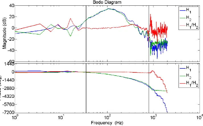
By applying a random noise on input 𝑛(𝑡) and assuming 𝑢(𝑡) = 0 the acoustic paths 𝐻1 and 𝐻2 can be

measured. The range of the random noise generator is set from 1 → 2000 𝐻𝑧, with 2000 𝐻𝑧 the Nyquist frequency of the sample frequency used in practice (will be explained in chapter IV). For now a sample frequency of 𝐹𝑠= 4000 𝐻𝑧 will be assumed. Both frequency responses of acoustic paths 𝐻1

and 𝐻2 are shown in Figure 6.

Figure 6: Frequency response 𝑯𝟏 and 𝑯𝟐

13 and a unreal response is measured. Both restrictions will determine the useful frequency response range by 35 − 800 𝐻𝑧, visible as the area between the two black lines.

R

In Figure 6 several resonance frequencies are visible, at for example 106 𝐻𝑧 which shows the largest magnitude of the acoustic air duct. Six clearly visible resonance frequencies can be obtained from Figure 6.

106 𝐻𝑧 136 𝐻𝑧 346 𝐻𝑧 450 𝐻𝑧 590 𝐻𝑧 710 𝐻𝑧

Those frequencies are the resonance frequencies of the AC air duct and can be calculated theoretically according to Ref. [20]. The resonance frequency of a tube with a closed and an open end can be calculated by.

𝑓𝑛=

𝑛𝑐

4(𝑙 + 0.4𝑑𝑖)

(II-2)

Similar, the resonance frequency of a two-sided open tube, can be calculated by.

𝑓𝑛=

𝑛𝑐

2(𝑙 + 0.3𝑑𝑖)

(II-3)

The first 8 resonance frequencies of the whole air duct are calculated according to (II-2).

𝑓₁ 𝑓₂ 𝑓₃ 𝑓₄ 𝑓₅ 𝑓₆ 𝑓₇ 𝑓₈

35 𝐻𝑧 69 𝐻𝑧 𝟏𝟎𝟒 𝑯𝒛 𝟏𝟑𝟖 𝑯𝒛 173 𝐻𝑧 207 𝐻𝑧 242 𝐻𝑧 277 𝐻𝑧

In which the third and fourth resonance frequency do correspond to the first two visible frequencies. Since the damping part of the air duct introduces a small volume change in the air duct, the damping part can be seen as a two ended open air duct with length 𝑙𝑑.

The first 8 resonance frequencies of the damping part are calculated according to (II-3).

𝑓₁ 𝑓₂ 𝑓₃ 𝑓₄ 𝑓₅ 𝑓₆ 𝑓₇ 𝑓₈

117 𝐻𝑧 235 𝐻𝑧 𝟑𝟓𝟐 𝑯𝒛 𝟒𝟕𝟎 𝑯𝒛 𝟓𝟖𝟕 𝑯𝒛 𝟕𝟎𝟓 𝑯𝒛 822 𝐻𝑧 940 𝐻𝑧

14

A

𝐺

𝐺

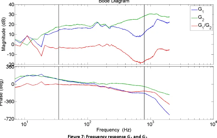
Similar measurements for acoustic paths 𝐺1 and 𝐺2 are provided. In this situation 𝑢(𝑡) will be the

random noise input and 𝑛(𝑡) = 0. The frequency responses are shown in Figure 7.

Figure 7: Frequency response 𝑮𝟏 and 𝑮𝟐

See the slightly higher magnitude of 𝐺2 compared to 𝐺1, introduced by the difference in distance

between the control speaker and microphones. Again, the black lines indicate the useful frequency range 35 − 800 𝐻𝑧. In practice we can say that the microphone outputs will never contain frequencies out of this frequency range introduced by the acoustic paths 𝐻1 and 𝐻2 and damped by the damping

part of the AC air duct. Except for unknown high frequency measurement noise the acoustic paths 𝐺1

and 𝐺2 are only exposed to frequencies within the useful frequency range. Since microphone output 2

is directly coupled to the input 𝑢(𝑡), by a given controller 𝐶, the useful frequency range of the controller is also equal to the frequency range obtained for 𝐻1 and 𝐻2.

P

By looking at the phase diagram for 𝐺1 and 𝐺2, a simple approximation of the distance between

microphone 1 and microphone 2 can be obtained. The distance in practice is given by 𝑙1− 𝑙2= 0.2 𝑚,

see Table 1. At the left boundary (35 𝐻𝑧) the phase of both acoustic paths is the same and equals approximately 90°. The phases at the right boundary (2000 𝐻𝑧) are given in Table 2.

Acoustic path Phase 𝒇 = 𝟑𝟓 𝑯𝒛 Phase 𝒇 = 𝟐𝟎𝟎𝟎 𝑯𝒛 Delta Phase

𝐺₁ 90° −636° 726°

𝐺₂ 90° −220° 310°

Table 2: Phase differences

The phase difference between both paths is 726 − 310 = 416° at 2000 𝐻𝑧. Corresponding to a frequency of 1731 𝐻𝑧 for a phase difference of 360°. By assuming a perfect sinusoidal sound wave traveling with the speed of sound, the length of this standing wave equals 343 1731⁄ ≈ 0.2 𝑚. Exactly equal to the measured distance between both microphones. Of course this is an approximation for

15 by the unsmooth behavior of the phase lines. Nevertheless, the result gives a practical feeling of phase delay introduced by the speed of sound travelling over a certain distance.

M

𝐹

𝐹

In practice the input signal 𝑒2(𝑡) of the controller will be filtered, idem for the output signal 𝑢(𝑡) of

the controller shown in Figure 5. This will be done to reduce the influence of noise in the system at frequencies out of the useful frequency range discussed before. For now, only the filters itself and the corresponding frequency responses will be discussed. Further information about the filters will be given in chapter IV.

Filter 𝐹1 is a self-made second order Butterworth filter with a cut-off frequency of 1125 𝐻𝑧. For details

about this self-made filter see appendix A.

Filter 𝐹2 is a Krohn-Hite model 3200 filter, known as a fourth order Butterworth filter, with a cut-off

frequency of 1000 Hz.

Both cut-off frequencies are chosen just above the right boundary of the useful frequency range of

800 𝐻𝑧. Measurements of the filters in practice are given in Figure 8.

Figure 8: Frequency response 𝑭𝟏 and 𝑭𝟐

According to [22], a second- and fourth order Butterworth filter can be written as a transfer function.

𝐹_{𝐵,2𝑛𝑑}= 𝜔

2

𝑠2_{+ √2𝜔𝑠 + 𝜔}2

(II-4)

𝜔4

𝑠4_{+ 2.61𝜔𝑠}3_{+ 3.41𝜔}2_𝑠2_{+ 2.61𝜔}3_{𝑠 + 𝜔}4

(II-5)

16

III

NOMINAL MODELS

All six frequency response models, from chapter II, will be identified to create corresponding nominal models of the acoustic paths. These nominal models will be used to design a controller and simulate Set up 2 in SIMULINK.

Two nominal models are already known and given by the Butterworth filter representations in chapter II. Both models fit well, see Figure 8. In text an additional ‘roof’ symbol will indicate the nominal model of a measured model in practice. In figures and illustrations an additional ‘nominal’ or ‘measurement’ term is added to distinguish between nominal and measured models.

𝐹̂₁ = 𝐹_{𝐵,2𝑛𝑑}

(III-1)

(III-2)

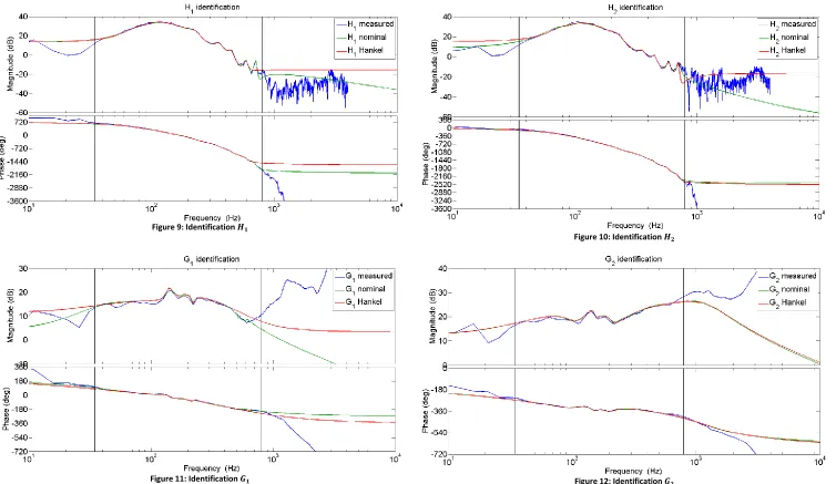
Frequency response identifications of the four remaining models is provided with the MATLAB command invfreqs and the results are shown in Figure 9 - Figure 12. All models are stable models, as required, and the fitted model order is given in Table 3. By using the invfreqs command only high order nominal models turn out to be stable and a good fit, but the complexity of the frequency response is not always that high. To reduce the order of the nominal models and keep the stability and complexity of the frequency response as good as possible, a Hankel order reduction will be used, according to Ref. [5]. These Hankel reduced nominal models will be used as the best nominal representation of the measured models in practice and are also shown in the figures by a red line.

Model Order invfreqs Order Hankel

𝐻̂1 25 16

𝐻̂₂ 24 16

𝐺̂1 22 9

𝐺̂₂ 21 9

17

Figure 9: Identification 𝑯𝟏

Figure 10: Identification 𝑯𝟐

18

IV

PRACTICE

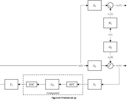
To design a stabilizing controller 𝐶, as shown in Set up 2 Figure 5, a practical set up will be created representing the situation in practice as good as possible. A schematic overview of the situation in practice is given in Figure 13 by adding both filters 𝐹1 and 𝐹2 and a computer block to the already

known Set up 2 of Figure 5. Filter 𝐹2 will be used to get rid of high frequency disturbances in the input

of the controller and filter 𝐹1 will cut-off the control signal of the control speaker. In practice the

zero-order-hold sampling of the computer will introduce a sound in the control signal equal to the sample frequency. Filter 𝐹1 is placed after the computer’s DAC conversion to cancel this sample frequency in

the control signal. Because of discrete time conversion by the computer (ADC), the designable controller must be a discrete time model as well, say 𝐶𝐷.

Figure 13: Practical set up

Obtain equations for 𝐶𝑖, 𝑢(𝑡), 𝑒1(𝑡) and 𝑒2(𝑡) using the practical set up in Figure 13.

𝐶_𝑖= 𝐷𝐴𝐶 ∙ 𝐶_𝐷∙ 𝐴𝐷𝐶

_(IV-1)

𝑢(𝑡) = 𝐹₂𝐶_𝑖𝐹₁𝑒₂(𝑡)

_(IV-2)

𝑒₁(𝑡) = (𝐻₁+ 𝐻₂ 𝐺1𝐹2𝐶𝑖𝐹1

1 − 𝐺₂𝐹₂𝐶_𝑖𝐹₁) 𝑛(𝑡)

(IV-3)

𝐻₂

19

F

Both real-time filters are already discussed in chapter II and nominal models, using the Butterworth representations, are given by 𝐹̂1 and 𝐹̂2. By looking at Figure 8 the magnitude of both filters is unity in

the useful frequency range so the filters will not influence the amplitude of the input and output signals for frequencies < 1000 𝐻𝑧. On the other side, both filters do introduce a small phase shift, especially in the higher frequency part of the useful frequency range. This will influence the stability of the system with the new closed loop gain in practice according to 𝐿 = −𝐺2𝐹2𝐶𝑖𝐹1, see (IV-4) . The stability criteria

will stay the same but the expression changed and will include more delay at higher frequencies introduced by 𝐹1 and 𝐹2. This will result into a smaller effective range of the controller and worse

performance of the system but both filters are necessary to get rid of unwanted high frequencies.

S

The computer in practice must be able to measure the useful frequency range 35 − 800 𝐻𝑧. To make sure that a frequency of 800 𝐻𝑧 will be picked up by the computer a sample frequency of 5 times the right boundary of the useful frequency range will be used.

𝐹𝑠= 5 ∗ 800 = 4000 𝐻𝑧

(IV-5)

𝑇𝑠=

1

𝐹_𝑠= 0.00025 𝑠

(IV-6)

C

The computer block in Figure 13 represents the connection of input microphone 2 and output control speaker signal 𝑢(𝑡). For this connection a National Instruments SCB-68desktop connector block [10] is used. Both ADC and DAC conversions of this connector block can be done within 0.01 𝑚𝑠 corresponding to a conversion frequency of 𝑓𝑐= 100 𝑘𝐻𝑧. For now the conversion time will be

neglected and the ADC and DAC conversions will assumed to be small in comparison to the calculation time of the controller for each sample. To make sure that the controller output is expectable the discrete controller 𝐶𝐷 cannot have a feedthrough term. In other words, the D-matrix of the state space

representation of 𝐶𝐷 equals zero. By using this restriction the whole ADC, DAC and discrete time

conversion of the controller, say the computer block, can be replaced by a zero-order-hold in continuous time with a continuous controller 𝐶 according to.

20

N

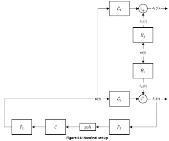
Using a continuous representation of the discrete computer block, the practical set up can be written as a continuous set up with only continuous nominal models, see Figure 14.

Figure 14: Nominal set up

The zero-order-hold term can be calculated using the sample time in (IV-6), according to.

𝑧𝑜ℎ = exp (−𝑇_𝑠∙ 𝑠)

_(IV-8)

Substitute (IV-7) into (IV-2) - (IV-4) to obtain the nominal equations for 𝑢(𝑡), 𝑒1(𝑡) and 𝑒2(𝑡).

𝑢̂(𝑡) = 𝐹̂₂∙ 𝑧𝑜ℎ ∙ 𝐶𝐹̂₁𝑒̂₂(𝑡)

(IV-9)

𝑒̂₁(𝑡) = (𝐻̂1+ 𝐻̂2

𝐺̂1𝐹̂2∙ 𝑧𝑜ℎ ∙ 𝐶𝐹̂1

1 − 𝐺̂2𝐹̂2∙ 𝑧𝑜ℎ ∙ 𝐶𝐹̂1

) 𝑛(𝑡)

(IV-10)

𝑒̂2(𝑡) =

𝐻̂₂

1 − 𝐺̂₂𝐹̂₂∙ 𝑧𝑜ℎ ∙ 𝐶𝐹̂₁𝑛(𝑡)

(IV-11)

With 𝑛(𝑡) the unknown input signal. The nominal closed loop gain 𝐿̂ and nominal sensitivity 𝑆̂ are given by.

𝑆̂ = 1

1 − 𝐺̂₂𝐹̂₂∙ 𝑧𝑜ℎ ∙ 𝐶𝐹̂₁

(IV-12)

(IV-13)

21

V

LOOP SHAPED CONTROLLER

Loop shaping is the first method used to create a controller satisfying the stability criteria. To obtain noise reduction, the sensitivity function 𝑆̂ must be as small as possible.

𝑆̂ = 1

1 + 𝐿̂→ 𝑠𝑚𝑎𝑙𝑙

(V-1)

Similar to an as large as possible closed loop gain.

𝐿̂ → 𝑙𝑎𝑟𝑔𝑒

(V-2)

At the same time, stability must be accomplished. Increasing the closed loop gain is possible but must fulfill the third stability criterion, known as.

∠(𝐿̂) ≠ ±180° 𝑖𝑓 |𝐿̂| ≥ 1.

(V-3)

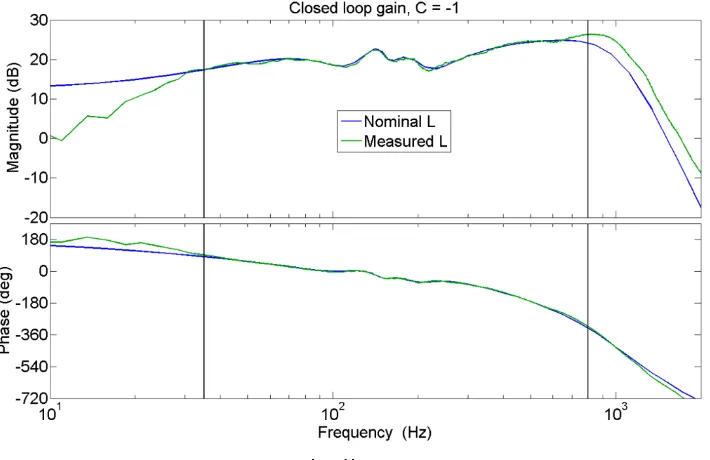
To see how the nominal models and the zero-order-hold term in the nominal closed loop expression (IV-13) do already influence the stability criterion, a frequency response of the nominal closed loop gain is created assuming 𝐶 = 1 and a sample frequency of 𝑓𝑠= 1 𝑇⁄ = 4000 𝐻𝑧𝑠 , see Figure 15.

Figure 15: Closed loop gain, 𝑪 = 𝟏

𝐶 = 1 is definitely not satisfying the stability criteria and results in an unstable nominal sensitivity. The magnitude is larger than unity in the useful frequency range and passes a phase of −180° in the middle of this range. In short, 𝐶 = 1 does not satisfy the stability criteria.

22

Figure 16: Closed loop gain, 𝑪 = −𝟏

Stable up to say 500 𝐻𝑧. For low frequencies the stability margin is very small and for frequencies around 500 𝐻𝑧 the nominal sensitivity function is unstable. What if a controller with a low gain in the low frequency region and a low gain in the frequency region around 500 𝐻𝑧 is introduced? This will increase the phase margin for low frequencies and reduce the gain below unity for frequencies above

500 𝐻𝑧. An example of such a controller is the following second order controller shown in (V-4). A zero is placed just before the useful frequency range, say 1 𝐻𝑧, to introduce a slope of +1. Followed by two poles at the frequency were the phase in Figure 16 is approximately zero, say 130 𝐻𝑧, to obtain a slope of −1. Ending with a slope of −1 introduces a zero feedthrough term and zero D-matrix in the state space representation. Which is a restriction for the controller if we use the nominal set up with a zero-order-hold term instead of a discrete computer block, all explained in chapter IV.

𝐶 = −𝑘 𝑠 + 𝜔1 𝑠2_{+ 2𝜁𝜔}

2𝑠 + 𝜔22

(V-4)

𝜔₁ = 1 𝐻𝑧 𝜔₂= 130 𝐻𝑧 𝜁 = 0.3 𝑘 = 45

23

Figure 17: Loop shaped controller

Figure 18: Closed loop gain, Loop shaped controller

The idea was to reduce the magnitude in the higher frequency part. As you can see the magnitude at higher frequencies is reduced and satisfies the stability criteria. Two intersections of phase ±180° can be see, one at 30 𝐻𝑧 and a second one at approximately 360 𝐻𝑧. For both intersections the stability criteria is satisfied because the corresponding magnitude is smaller than unity (< 0 𝑑𝐵).

P

To see the performance in practice and the correctness of the nominal model 𝐶 ∗ 𝑧𝑜ℎ, the controller is discretized and used in the computer block as shown by 𝐶𝐷 in Figure 13. Before the outputs 𝑒2(𝑡)

and 𝑒1(𝑡) are measured, the correctness of 𝑧𝑜ℎ ∗ 𝐶, as a model for the computer block 𝐴𝐷𝐶 ∗ 𝐶𝐷∗

24

Figure 19: Check Controller

As expected the 𝑧𝑜ℎ ∗ 𝐶 representation of the computer block 𝐴𝐷𝐶 ∗ 𝐶𝐷∗ 𝐷𝐴𝐶 is correct. Controller

𝐶_𝐷 is calculated with the MATLAB command 𝑐2𝑑(𝐶, 𝑇𝑠, 𝑧𝑜ℎ) using a zero-order-hold discretization method. Applying the discretized controller on the real system in practice, the outputs 𝑒1(𝑡) and 𝑒2(𝑡)

can be measured. A random noise signal with a frequency range of 0 → 2 𝑘𝐻𝑧 is applied at input 𝑛(𝑡) and the frequency response calculated by the Control systems analyzer is visible as the cyan lines in Figure 20 and Figure 21.

S

A stabilizing controller (V-4) is designed by loop shaping the nominal closed loop gain. By simulating the outputs 𝑒1(𝑡) and 𝑒2(𝑡) using a random noise input 𝑛(𝑡), the performance of the controller can

be seen. By looking at Figure 18 the best performance is expected around 130 𝐻𝑧 were the phase is

0°. The worst performance, or maybe even an increase in amplitude, is expected at the intersections with phase ±180°, known by the frequencies 30 𝐻𝑧 and 360 𝐻𝑧. The result is shown in Figure 20 and Figure 21 for output 𝑒1(𝑡) and 𝑒2(𝑡) respectively. How the nominal models are implemented in

25

Figure 20: Output 𝒆𝟏(𝒕), Loop shaped controller

Figure 21: Output 𝒆𝟐(𝒕), Loop shaped controller

As you can see, the nominal setup including nominal models and a nominal controller (red line) or the light blue line, using the measured models instead of nominal models and the nominal controller, do show a good fit compared to the frequency response in practice (cyan line). Incoming sound is reduced in the frequency range 70 − 170 𝐻𝑧 with a maximum magnitude ratio of 0.45 around 130 𝐻𝑧 as expected. A worse performance and even an increase in magnitude as expected around 300 𝐻𝑧 is correct as well. (control lines above no control lines in Figure 21).

In short, the amount of noise reduction in practice is similar to the nominal models used to create the loop shaped controller but the total amount of noise reduction is small. Using a loop shaped static second order controller will result into a stable feedback system with sound reduction but the amount is almost neglectable. In chapter VI an 𝐻2 controller will be designed to see if such a controller can do

26

VI

𝐻

₂

CONTROLLER

According to [4], [7] and [8], the 𝐻2 control problem can be presented in the following way.

Introduce the partition of 𝑇 according to.

[𝑒̂_𝑒̂1(𝑡)

2(𝑡)] = [

𝑇₁₁ 𝑇₁₂ 𝑇21 𝑇22] [

𝑛(𝑡)

𝑢̂(𝑡)]

(VI-1)

The closed loop transfer function 𝐹(𝑇, 𝐶𝐻) is given as.

𝐹(𝑇, 𝐶𝐻) = 𝑇11+ 𝑇12(𝐼 − 𝐶𝐻𝑇22)−1𝐶𝐻𝑇21

(VI-2)

𝑒̂₁(𝑡) = 𝐹(𝑇, 𝐶_𝐻)𝑛(𝑡)

(VI-3)

This 𝐻2 control problem consists of finding a controller 𝐶𝐻 which stabilizes the plant 𝑇 and minimizes

the following cost function.

𝐽(𝐶𝐻) = ‖𝐹(𝑇, 𝐶𝐻)‖22

(VI-4)

With ‖𝐹(𝑇, 𝐶𝐻)‖2 the 𝐻2-norm.

The problem is most conveniently solved in the time domain and assumed will be the state-space representation of plant 𝑇.

𝑥(𝑡) = 𝐴𝑥(𝑡) + 𝐵1𝑛(𝑡) + 𝐵2𝑢(𝑡)

(VI-5)

𝑒̂₁(𝑡) = 𝐶₁𝑥(𝑡) + 𝐷₁₁𝑛(𝑡) + 𝐷₁₂𝑢(𝑡)

_(VI-6)

(VI-7)

In the state-space representation 𝐷22= 0. The direct feedthrough from 𝑢(𝑡) to 𝑒̂2(𝑡) has assumed to

be zero because physical systems always have a zero gain at infinite frequency. In our case this is not true because the nominal models 𝐺̂1 and 𝐺̂2, representing the physical system, do have a small

feedthrough term as can be seen as a zero-slope in Figure 11 and Figure 12 for high frequencies. According to Ref. [7] an optimal controller does not exist if 𝐷12 does not have full column rank or 𝐷21

does not have full row rank. In both situations solving the Ricatti equation, the method to obtain controller 𝐶𝐻 by minimizing the cost function, is not possible because of control singularity or sensor

27

I

Implement the nominal set up as given in Figure 14, in which the closed loop transfer function is a representation of the transfer function between output 𝑒̂1(𝑡) and input 𝑛(𝑡) in (IV-10).

𝐹(𝑇, 𝐶𝐻) = 𝑇11+ 𝑇12(𝐼 − 𝐶𝐻𝑇22)−1𝐶𝐻𝑇21

(VI-8)

𝑒̂₁(𝑡) = 𝑇11𝑛(𝑡) + 𝑇12𝑢̂(𝑡)

(VI-9)

𝑒̂₂(𝑡) = 𝑇21𝑛(𝑡) + 𝑇22𝑢̂(𝑡)

(VI-10)

𝑢̂(𝑡) = 𝐶_𝐻𝑒̂₂(𝑡)

(VI-11)

The following T-matrix can be assumed.

𝑇11= 𝐻̂1

(VI-12)

(VI-13)

𝑇21= 𝐻̂2

(VI-14)

(VI-15)

Rewrite (VI-9) and (VI-10) by substituting (VI-11) - (VI-15).

𝑒̂1(𝑡) = (𝐻̂1+ 𝐻̂2

𝐺̂₁𝐶_𝐻

1 − 𝐺̂₂𝐶_𝐻) 𝑛(𝑡)

(VI-16)

1 − 𝐺̂₂𝐶_𝐻𝑛(𝑡)

(VI-17)

In which 𝐶𝐻 will be the 𝐻2 controller found by minimizing the cost function.

Problem 1:

The nominal expressions 𝑢̂(𝑡) in the nominal set up is already given in (IV-9) and must be equal to (VI-11) above to make 𝐶𝐻 usable as the representation of controller 𝐶 in the nominal set up.

𝑢̂(𝑡) = 𝑧𝑜ℎ ∙ 𝐶𝐹̂₁𝑒̂₂(𝑡) = 𝐶_𝐻𝑒̂₂(𝑡)

(VI-18)

(VI-18) implies that a 𝐶𝐻 controller will correspond to the 𝑧𝑜ℎ ∙ 𝐶𝐹̂1 term in the nominal model. So the

𝐶_𝐻 controller is not directly related to 𝐶 and not implementable in the computer block.

Solution 1a:

The nominal controller can be calculated by dividing the 𝐻2 controller 𝐶𝐻 by the filter 𝐹̂1 and

zero-order-hold term 𝑧𝑜ℎ.

𝑧𝑜ℎ ∙ 𝐶𝐹̂₁= 𝐶_𝐻→ 𝐶 = 𝐶𝐻

𝑧𝑜ℎ ∙ 𝐹̂₁

(VI-19)

In which 𝑧𝑜ℎ−1= exp (𝑇𝑠∙ 𝑠) is a non-existing function, so the calculation will not be possible.

Solution 1b:

Implement the two filters and zero-order-hold term into the plant 𝑇 instead of the assumptions for the T-matrix above in

(VI-12)

28

𝐹(𝑇, 𝐶_𝐻) = 𝑇11+ 𝑇12(𝐼 − 𝐶𝐻𝑇22)−1𝐶𝐻𝑇21= 𝐻̂1+ 𝐻̂2

𝐺̂₁𝐹̂₂∙ 𝑧𝑜ℎ ∙ 𝐶𝐹̂₁

1 − 𝐺̂₂𝐹̂₂∙ 𝑧𝑜ℎ ∙ 𝐶𝐹̂₁

(VI-20)

Obtain the three unknown terms in (VI-20).

𝑇₁₁= 𝐻̂₁

(VI-21)

(VI-22)

(VI-23)

Check the output equations:

𝑢̂(𝑡) = 𝐶_𝐻𝑒̂₂(𝑡)

(VI-24)

𝑒̂₁(𝑡) = 𝑇₁₁𝑛(𝑡) + 𝑇₁₂𝑢̂(𝑡) = 𝐻̂₁+ 𝑇₁₂𝐶_𝐻𝑒̂₂(𝑡)

(VI-25)

𝑒̂₂(𝑡) = 𝑇21𝑛(𝑡) + 𝐺̂2𝐹̂2∙ 𝑧𝑜ℎ ∙ 𝐹̂1𝐶𝐻𝑒̂2(𝑡) → 𝑒̂2(𝑡) =

𝑇₂₁

1 − 𝐺̂2𝐹̂2∙ 𝑧𝑜ℎ ∙ 𝐹̂1𝐶𝐻

𝑛(𝑡)

_(VI-26)

By looking at the nominal equation for 𝑒̂2(𝑡) in (IV-11) we can see that 𝑇21= 𝐻̂2.

Substitute into

(VI-22)

𝑇12𝐻̂2= 𝐻̂2𝐺̂1𝐹̂2∙ 𝑧𝑜ℎ ∙ 𝐹̂1→ 𝑇12= 𝐺̂1𝐹̂2∙ 𝑧𝑜ℎ ∙ 𝐹̂1

(VI-27)

Substitute (VI-26) and (VI-27) into (VI-25).

𝑒̂₁(𝑡) = (𝑇11+ 𝑇21

𝑇12𝐶𝐻

1 − 𝑇22) 𝑛(𝑡) = 𝐻̂1𝑛(𝑡) + 𝐻̂2

𝐺̂1𝐹̂2∙ 𝑧𝑜ℎ ∙ 𝐹̂1𝐶𝐻

1 − 𝐺̂2𝐹̂2∙ 𝑧𝑜ℎ ∙ 𝐹̂1𝐶𝐻

𝑛(𝑡)

(VI-28)

Which is identical to the 𝑒̂1(𝑡) in (IV-10) using the following components of plant 𝑇.

𝑇₁₁= 𝐻̂₁

(VI-29)

(VI-30)

𝑇₂₁= 𝐻̂₂

(VI-31)

(VI-32)

29

Figure 22: Nominal set up, partition 𝑻

Problem 2:

By substituting the filters 𝐹̂2 and 𝐹̂1 into 𝑇12 the feedthrough term of 𝑇12 becomes zero. Introduced by

the fact that the feedthrough term of a Butterworth filter is always zero (ending negative slope). This results into 𝐷12= 0 for plant 𝑇, making it impossible to solve the Ricatti equation as well as finding a

controller 𝐶𝐻.

Solution 2:

By adding 𝑛-zeros to the filters 𝐹1 and 𝐹2 at a very high frequency 𝜔ℎ𝑖𝑔ℎ, the ending negative slope

can be flattened for very high frequencies. This results into a non-zero feedthrough term for 𝜔 → ∞ and will get rid of the control singularity problem. Both filters will be replaced by the following equation with 𝑛 the order of the Butterworth filter and 𝜔ℎ𝑖𝑔ℎ a selectable high frequency, say 10 times the

cut-off frequency of the filters.

𝐹_𝑛𝑒𝑤 = 1

𝜔_{ℎ𝑖𝑔ℎ}𝑛 𝐹(𝑠 + 𝜔ℎ𝑖𝑔ℎ) 𝑛

(VI-33)

C

𝐶

Now the singularity issues are solved and the 𝐶𝐻 controller can be discretized and implemented

directly in the computer block, the 𝐶𝐻 controller can be calculated solving the Ricatti equations with

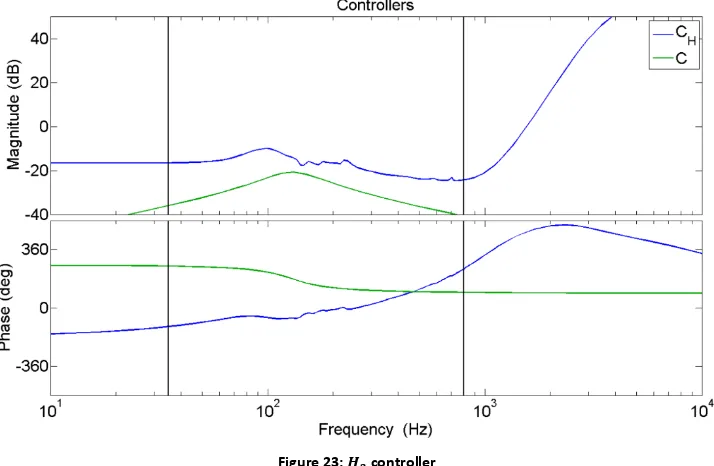
30 The result of this calculation is shown in Figure 23. 𝐶𝐻 stabilizes the nominal sensitivity function 𝑆̂ but

is unstable itself. Since the first stability criterion demands a stable closed loop gain, the controller itself must be stable too.

Figure 23: 𝑯𝟐 controller

A second figure will show the frequency response of the closed loop transfer function also known by the output 𝑒̂1(𝑡), see Figure 24.

Figure 24: Output 𝒆𝟏(𝒕), 𝑯𝟐 controller

A nice result but not usable in practice because the controller itself is unstable. You can see the very nice behavior of the 𝐻2 controller in the phase diagram of Figure 23. Phase increases by increasing the

frequency as an opposite response of acoustic path 𝐺2, see Figure 12. That way, the closed loop gain

31

32

VII

YOULA CONTROLLER SET UP 2

Another way of improving the sound reduction is using a real-time updating controller. By shaping the controller, based on the characteristics of the incoming noise 𝑛(𝑡), the sound can be reduced even more. Again, the controller must satisfy the three stability criteria and according to the first stability criterion the controller must always be stable 𝐶 ∈ ℛℋ∞. This can be achieved by using a Youla

parameterization according to Ref. [15].

Y

According to chapter VI the closed loop transfer function of the nominal set up can be written as.

[𝑒̂1(𝑡) 𝑒̂2(𝑡)] = [

𝑇11 𝑇12

𝑇₂₁ 𝑇₂₂] [𝑛(𝑡)𝑢̂(𝑡)]

(VII-1)

With the T-matrix given by.

𝑇₁₁= 𝐻̂₁

(VII-2)

(VII-3)

𝑇₂₁= 𝐻̂₂

(VII-4)

(VII-5)

Consider the feedback system for nominal output 𝑒̂2(𝑡) and neglect output 𝑒̂1(𝑡) for now.

𝑒̂2(𝑡) = 𝑇22𝑢̂(𝑡) + 𝑇21𝑛(𝑡)

(VII-6)

𝑢̂(𝑡) = 𝐶𝑒̂2(𝑡)

(VII-7)

Assume 𝐶 = −𝐶𝑖 to obtain a negative feedback loop, which will be easier for writing down the Youla

parameterization further on.

𝑢̂(𝑡) = −𝐶_𝑖𝑒̂₂(𝑡)

(VII-8)

𝑒̂₂(𝑡) = 𝑇21

1 + 𝑇22𝐶𝑖𝑛(𝑡)

(VII-9)

Y

U

Consider the feedback connection of a nominal model 𝑇22 and initial controller 𝐶𝑖 stabilizing the closed

loop transfer function 𝑃(𝐶𝑖, 𝑇22) ∈ ℛℋ∞.

𝑃(𝐶_𝑖, 𝑇₂₂) = [𝐶𝑖

𝑇₂₂] (𝐼 + 𝑇22𝐶𝑖)−1[𝑇22 𝐼]

(VII-10)

All 𝐶𝑄 = 𝑁𝑄𝐷𝑄−1 that satisfy 𝑃(𝐶𝑄, 𝑇22) ∈ ℛℋ∞ are given by the right-coprime-factorization (rcf) and

Youla parameter 𝑄 according to.

𝑁𝑄 = 𝑁𝑖+ 𝐷𝑄

(VII-11)

𝐷𝑄 = 𝐷𝑖− 𝑁𝑄

(VII-12)

33 With the rcf 𝑇22= 𝑁𝐷−1 and 𝐶𝑖 = 𝑁𝑖𝐷𝑖−1 according to Ref. [3]. In which the left-coprime-factorization

(lcf) is given as 𝑇22= 𝐷̃−1𝑁̃ and 𝐶𝑖 = 𝐷̃𝑖−1𝑁̃𝑖. When 𝑄 is stable, stability can be obtained for the

feedback of 𝐶𝑄 and 𝑇22. Using coprime factorization to formulate stability of a feedback connection of

𝐶_𝑖 and 𝑇22 as 𝑃(𝐶𝑖, 𝑇22) ∈ ℛℋ∞ for internal stability, is equivalent to Λ−1∈ ℛℋ∞.

Λ = 𝐷̃𝐷_𝑖+ 𝑁̃𝑁_𝑖

(VII-14)

The Youla Controller can be obtained from the rcf 𝐶𝑄 = 𝑁𝑄𝐷𝑄−1.

𝐶_𝑄 = (𝑁_𝑖+ 𝐷𝑄)(𝐷_𝑖− 𝑁𝑄)−1

(VII-15)

T

If nominal plant 𝑇22 and stabilizing controller 𝐶𝑖 are stable, a trivial choice for the rcf representations

will be.

𝐷̃ = 𝐷 = 𝐼 𝐷̃_𝑖 = 𝐷_𝑖 = 𝐼 𝑁̃ = 𝑁 = 𝑇₂₂ 𝑁̃_𝑖 = 𝑁_𝑖 = 𝐶_𝑖

Substitute into (VII-14) and (VII-15).

𝐶_𝑄= (𝐶_𝑖+ 𝑄)(𝐼 − 𝑇₂₂𝑄)−1

_(VII-16)

22𝐶𝑖

(VII-17)

R

S

2

A schematic representation of the Youla Controller is given in Figure 26 and implemented in Set up 2 as shown in Figure 27.

𝑒̂₂(𝑡) = 𝑇₂₂𝑢̂(𝑡) + 𝑇₂₁𝑛(𝑡)

_(VII-18)

𝑢̂(𝑡) = −𝐶𝑄𝑒̂2(𝑡)

(VII-19)

34

Figure 27: Youla parameterization Set up 2

Our goal is to minimize the output 𝑒̂2(𝑡) according to Set up 2 and stabilize the nominal sensitivity

satisfying the stabilizing criteria. To do so, the approach of Set up 2 minimizes the following weighted two-norm performance measure.

‖𝛾𝑊𝑢̂(𝑡)_𝑒̂

2(𝑡) ‖2

(VII-20)

Where 𝑊 is a user-specified monic stable filter to satisfy the stability criteria, and 𝛾 is an additional scalar weighting allowed because of the monicity of 𝑊.

The variance of 𝑒̂2(𝑡) and 𝑢̂(𝑡) is driven by the input 𝑛(𝑡) and nominal model 𝑇21 in which 𝑛(𝑡) is an

unknown noise signal, see (VII-18). The Youla parameterization allows the weighted two-norm to be written as a function of the stable Youla parameter 𝑄.

L

Q

To write the two-norm as a function of 𝑄 the Youla controller in (VII-15) is substituted into both terms of the performance measure in (VII-20).

𝛾𝑊𝑢̂(𝑡) = −𝛾𝑊(𝑁_𝑖+ 𝐷𝑄)(𝐷_𝑖− 𝑁𝑄)−1_𝑒̂

2(𝑡)

(VII-21)

𝑒̂₂(𝑡) =_{1 + 𝑁𝐷−1} 𝑇21

(𝑁𝑖+ 𝐷𝑄)(𝐷𝑖− 𝑁𝑄)−1𝑛(𝑡)

(VII-22)

Rewrite (VII-22).

𝑒̂₂(𝑡) = 𝑇21𝐷𝑖−1

𝐷𝑖− 𝑁𝑄

𝐼 + 𝑁𝐷−1_𝑁 𝑖𝐷𝑖−1

𝑛(𝑡)

_(VII-23)

Substitute (VII-23) into (VII-21).

𝛾𝑊𝑢̂(𝑡) = −𝛾𝑊𝑇₂₁𝐷_𝑖−1_{(𝐼 + 𝑁𝐷}−1_𝑁 𝑖𝐷𝑖−1)

−1

35 (VII-23) and (VII-24) can be written as a vector summation linear in 𝑄.

[𝛾𝑊𝑢̂(𝑡)_𝑒̂

2(𝑡) ] = [

−𝛾𝑊𝑁_𝑖

𝐷_𝑖 ] 𝑤(𝑡) − [𝛾𝑊𝐷𝑁 ] 𝑄𝑤(𝑡)

(VII-25)

With 𝑤(𝑡) according to.

𝑤(𝑡) = 𝑇₂₁𝐷_𝑖−1(𝐼 + 𝑇₂₂𝐶_𝑖)−1_𝑛(𝑡)

_(VII-26)

𝑇21𝑛(𝑡) can be obtained from the signals −𝑒̂2(𝑡) and 𝑢̂(𝑡). By using coprime factorizations and a

stabilizing controller 𝐶𝑖, the signal 𝑤(𝑡) is more general than an output or equation error observer of

the nominal disturbance signal 𝑣̂2(𝑡). Obtain 𝑇21𝑛(𝑡) from (VII-6) by rewriting the equation.

𝑒̂2(𝑡) = 𝑇22𝑢̂(𝑡) + 𝑇21𝑛(𝑡) → 𝑇21𝑛(𝑡) = 𝑒̂2(𝑡) − 𝑇22𝑢̂(𝑡)

(VII-27)

Can be written as a vector multiplication.

𝑇₂₁𝑛(𝑡) = [𝑇22 𝐼] [−𝑢̂(𝑡)_𝑒̂

2(𝑡) ]

(VII-28)

Substitute (VII-28) into (VII-26).

𝑤(𝑡) = 𝐷_𝑖−1(𝐼 + 𝑇22𝐶𝑖)−1[𝑇22 𝐼] [−𝑢̂(𝑡)_𝑒̂ 2(𝑡) ]= Λ

−1_{[𝑁̃ 𝐷̃] [}−𝑢̂(𝑡)

𝑒̂2(𝑡) ]

(VII-29)

Based on this analysis, the filtered closed loop signal 𝑤(𝑡) can be defined with Λ−1∈ ℛℋ∞,

𝑃(𝐶_𝑖, 𝑇₂₂) ∈ ℛℋ∞ and 𝑇22∈ ℛℋ∞. Proof for (VII-29) is given in appendix B.

By allowing a parameterization of 𝑄(𝜃), the error signal will be linear in the parameter 𝜃, if and only if 𝑄(𝜃) ∈ ℛℋ∞ is parameterized linearly in the parameter 𝜃.

‖𝛾𝑊𝑢̂(𝑡)

𝑒̂2(𝑡) ‖₂= lim𝑁→∞

1

𝑁∑ 𝜀(𝑡, 𝜃)𝑇𝜀(𝑡, 𝜃)

𝑁

𝑡=1

(VII-30)

𝜀(𝑡, 𝜃) = [−𝛾𝑊𝑁_𝐷 𝑖

𝑖 ] 𝑤(𝑡) − [𝛾𝑊𝐷𝑁 ] 𝑄(𝜃)𝑤(𝑡)

(VII-31)

FIR

An obvious choice for 𝑄(𝜃), according to Ref. [11], is an FIR model of order 𝑛. Given the FIR property of inherent stability, with all poles located at the origin, will introduce an always stable model for 𝑄.

𝑄(𝑞, 𝜃) = 𝜃₀+ ∑ 𝜃_𝑘𝑞−𝑘 𝑛

𝑘=1

(VII-32)

36

U

The error signal optimization is based on all time samples from 𝑁 = 1 → ∞ in which updating the controller is only possible after a finite measurement. To anticipate changes in the frequency spectrum of 𝑛(𝑡), the error signal optimization is computed over a finite number of time samples.

𝜃̂_𝑡 = min

𝜃

1

𝑡∑ 𝜀(𝜏, 𝜃)𝑇𝜀(𝜏, 𝜃)

𝑡

𝜏=0

(VII-33)

This finite time computation is used to formulate a Recursive Least Squares (RLS) solution as in [13].

For a SISO system the expression for the error signal in (VII-31) can be simplified.

𝜀(𝑡, 𝜃) = 𝑦𝑓(𝑡) − 𝑄(𝜃)𝑢𝑓(𝑡)

(VII-34)

Where 𝑦𝑓(𝑡) denotes the filtered output and 𝑢𝑓(𝑡) the filtered input signal.

𝑦_𝑓(𝑡) = [−𝛾𝑊𝑁𝑖

𝐷_𝑖 ] 𝑤(𝑡)

(VII-35)

(VII-36)

For a linearly parameterized scalar 𝑄(𝑞, 𝜃), the error signal 𝜀(𝑡, 𝜃) can be written in a linear regression form with a regressor 𝜙(𝑡). Where the regressor contains past versions of the input signal 𝑢𝑓(𝑡).

𝜀(𝑡, 𝜃̂𝑡) = 𝑦𝑓(𝑡) − 𝜙(𝑡)𝑇𝜃̂𝑡

(VII-37)

𝜙(𝑡)𝑇 _{= [𝑢}

𝑓(𝑡) 𝑢𝑓(𝑡 − 1) … 𝑢𝑓(𝑡 − 𝑛)]

(VII-38)

A standard RLS update algorithm in [23] and [24] can be summarized by three iterative steps. 1) Prediction error update

𝜀(𝑡, 𝜃̂𝑡−1) = 𝑦𝑓(𝑡) − 𝜙(𝑡)𝑇𝜃̂𝑡−1

(VII-39)

2) Weighted covariance update

𝑃_𝑡 = 𝑃_𝑡−1− 𝑃_𝑡−1𝜙(𝑡)[𝜙(𝑡)𝑇_𝑃

𝑡−1𝜙(𝑡) + 𝐼2×2 ]−1𝜙(𝑡)𝑇𝑃𝑡−1

(VII-40)

3) Parameter update

𝜃̂_𝑡 = 𝜃̂_𝑡−1+ 𝑃_𝑡𝜙(𝑡)𝜀(𝑡, 𝜃̂𝑡−1)

(VII-41)

C

To avoid convergence of the parameters 𝜃̂𝑡, when the covariance matrix 𝑃𝑡 → 0, a forgetting factor 𝜆

is added to the weighted covariance update in (VII-40) according to Ref. [24].

𝑃_𝑡 = 𝑃_𝑡−1𝜆−1_{− 𝑃}

𝑡−1𝜆−1𝜙(𝑡)[𝜙(𝑡)𝑇𝑃𝑡−1𝜙(𝑡) + 𝐼2×2 ]−1𝜙(𝑡)𝑇𝑃𝑡−1

(VII-42)

37 Adding the forgetting factor to the weighted covariance update will introduce an exponential weighting over the regressor. By choosing 𝜆 small, the contribution of the previous samples in the regressor will be small as well. This will make the filter sensitive to the newest samples in the regressor introducing a fast response to a major frequency change in the input.

S

The parameters 𝜃̂𝑡 are directly used in the controller perturbation 𝑄(𝑞, 𝜃̂𝑡 ) in (VII-32), introducing

major possible changes of the controller in the control signal 𝑢̂(𝑡) = −𝐶𝑄𝑒̂2(𝑡). To avoid large and

rapid changes of the control signal, the parameters 𝜃̂𝑡 will be time filtered before it is used in the

controller perturbation. The calculation of the time filtered parameters 𝜃̃𝑡 used in 𝑄(𝑞, 𝜃̃𝑡) is given by.

𝜃̃_𝑡 = (1 − 𝛿)𝜃̂_𝑡+ 𝛿𝜃̃_𝑡−1

(VII-43)

With 0 ≤ 𝛿 < 1. The closer 𝛿 is to 1, the more filtering and the slower the update of the controller.

F

W

To avoid updating of the controller for frequencies above the useful frequency range, the user-specified filter 𝑊 will be a model similar to the inverse of a low pass filter. By introducing a large gain for high frequencies in the 2-norm minimization via 𝛾𝑊𝑢̂(𝑡), the updating algorithm will try to reduce the gain for high frequencies to get rid off this massive gain in the first argument of the 2-norm, see (VII-20). In other words, It will ‘reduce’ the influence of high frequencies on the Youla Updating controller.

Similar for frequencies lower than the left boundary of the frequency range. By introducing a low pass filter the influence of low frequencies in the RLS algorithm will be less. Combining the high frequency inverse low pass filter and the low frequency low pass filter will result into a filter W with a high gain outside and a small gain inside the useful frequency range.

A possible fourth-order model for 𝑊, satisfying both boundaries, is shown in Figure 28 and given by.

𝑊 = 𝑧

4 _{− 2.945𝑧}3 _{+ 3.286𝑧}2 _{− 1.703𝑧 + 0.3628}

38

Figure 28: Filter W

S

Implementing the updating algorithm for controller 𝐶𝑄 into a SIMULINK model with all the nominal

models as given in chapter III, makes it possible to estimate the outputs 𝑒̂1(𝑡) and 𝑒̂2(𝑡) for an

unknown input 𝑛(𝑡). The results, for white noise input 𝑛(𝑡), are shown in Figure 29 and Figure 30 . A sample frequency of 4000 𝐻𝑧 in combination with a 15th _{order Youla parameter (𝑛 = 15) is used. The}

order of the controller is based on the calculation time of the Youla Updating algorithm on the computer in practice. By increasing the order of the controller the calculation time will increase as well. After some trial and error, the highest possible order, at a sample frequency of 4000 𝐻𝑧, equals 15. For 𝑛 = 16 the calculation time of the algorithm is larger than the sample time and the computer will crash. To make both simulation and practice comparable, the same sample frequency and model order will be used in SIMULINK as in practice.

39

Figure 30: Output 𝒆𝟐(𝒕) Set up 2, Youla Controller

Since the input is white noise the updating algorithm cannot really use its capabilities of updating the controller in time. The result is expected to be better than the nominal loop shaped controller but not that much. Comparing Figure 21 and Figure 30 or Figure 20 and Figure 29 the result is indeed similar but slightly better for the Youla Updating controller. Random noise is never the same for a small moment of time, so updating the controller with the time-filter for stability, will never result into a major controller change compared to the initial stabilizing controller 𝐶𝑖. One possible expected change

will be the gain of the controller which will be updated in the Youla Updating Controller to obtain the perfect gain for the situation. Since the gain of the loop shaped controller is chosen at the safe side, according to the stability criteria, the gain of the Youla controller is expected to be larger.

40

Figure 31: Youla Controller Set up 2

As expected the Youla Controller has a larger gain than the initial controller 𝐶𝑖. A high peak at the end

of the frequency domain is introduced by the FIR filter used to describe model 𝑄 as a stable model. By looking at the shape of the initial controller, compared to the two Youla Updating controllers, the controller shows similar behavior with a small gain in the lower frequency range, a higher gain in the frequency range 50 → 250 𝐻𝑧 and a negative slope for higher frequencies.

U

To see the updating performance of the algorithm a varying single sine input 𝑛(𝑡) is applied to see the response and capabilities of the Youla Updating controller 𝐶𝑄. Starting with a 80 𝐻𝑧 single sine for 5

41

Figure 32: Time output 𝒆𝟏(𝒕) Set up 2, single sine input 𝒏(𝒕)

Figure 33: Time output 𝒆𝟐(𝒕) Set up 2, single sine input 𝒏(𝒕)

The updating capabilities of the controller algorithm are clearly visible in both figures. When the frequency of the input changes (for example at 𝑡 = 5 𝑠) the error is large because the controller is still based on the previous input frequency. When the new samples are measured and the new frequency is coming into the regressor, the controller updates itself and reduces the new frequency. This behavior repeats itself for every major frequency change in the input 𝑛(𝑡).

Compare the red and green lines corresponding to the SIMULINK simulation and results in practice respectively. You can see similar lines for 𝑒1(𝑡) (green line in Figure 32) and 𝑒2(𝑡) (green line in Figure

33) in practice but the red lines in both figures are not that identical. The controller is calculated minimizing the 2-norm of output 𝑒2(𝑡), according to (VII-20), so more reduction is expected for output

42 can see the controller working on 𝑒2(𝑡) much better in the simulation than in practice but 𝑒1(𝑡) in the

simulation is worse than in practice. This is mainly introduced by unknown noise in practice not perfectly taken into account in the simulation. White noise is added to the simulation, see Figure 41, to see the behavior of noise on the stability of the Youla Updating controller but is not identical to the noise in practice.

By applying an input signal with only one major frequency a controller with the same dominant frequency is expected. A magnitude increase or peak at the input frequency is expected as a reaction of the Youla Updating controller to reduce that frequency. To see this behavior the FIR models of the controller are plotted for 𝑡 = 5, 10 and 15 just before the frequency change happens, see Figure 34.

Figure 34: Youla controller Set up 2, single sine input 𝒏(𝒕)

43

VIII

YOULA CONTROLLER GENERAL SET UP

In chapter 0 the Youla Controller approach is shown for input 𝑛(𝑡) and output 𝑒2(𝑡) according to Set

up 2. In practice the most outer microphone, corresponding to output 𝑒1(𝑡), will be the leading

microphone measuring the amount of acoustic noise cancellation. To improve the noise cancellation at output 𝑒1(𝑡) the updating Youla Controller can be written according to Set up 1 instead of Set up 2.

Unfortunately, the acoustic path 𝐺1 of Set up 1 introduces more delay and that decreases the

controllability of the system. The final results are even worse than using Set up 2 and simply measuring the output 𝑒1(𝑡) as in Figure 32. Another possibility is to use the system in Set up 2, but change the

Youla Updating controller into a minimizing 2-norm for output 𝑒1(𝑡) instead of 𝑒2(𝑡). This is the so

called ‘General Set up’.

Y

G

S

The closed loop transfer function 𝑇, Youla Controller 𝐶𝑄 and equations for the nominal outputs as

presented in chapter 0 will remain the same for the General Set up.

R

G

S

A schematic representation of the Youla Controller in the General Set up is given in Figure 35.

Figure 35: Youla parameterization General Set up

This time, our goal is to minimize the output 𝑒̂1(𝑡) and stabilize the nominal sensitivity according to

the stabilizing criteria for output 𝑒̂2(𝑡). To do so the approach of the General Set up minimizes the

following weighted two-norm performance measure.

‖𝛾𝑊𝑢̂(𝑡)_𝑒̂

44 The variance of 𝑒̂1(𝑡) and 𝑢̂(𝑡) is driven by the input 𝑛(𝑡) and nominal model 𝑇11 according to (VII-1),

in which 𝑛(𝑡) is an unknown noise signal. 𝑢̂(𝑡) is already given in (VII-8) and 𝑒̂1(𝑡) can be obtained

from (VII-1).

𝑒̂₁(𝑡) = 𝑇₁₂𝑢̂(𝑡) + 𝑇₁₁𝑛(𝑡)

_(VIII-2)

L

Q

G

S

The Youla parameterization allows the weighted 2-norm to be written as a function of the stable Youla parameter 𝑄. To write the 2-norm as a function of 𝑄, the Youla Updating controller in (VII-15), 𝑒̂1(𝑡)

in (VIII-2) and 𝑢̂(𝑡) in (VII-8) are substituted into both terms of the performance measure in (VIII-1).

𝛾𝑊𝑢̂(𝑡) = −𝛾𝑊(𝑁_𝑖+ 𝐷𝑄)(𝐷_𝑖− 𝑁𝑄)−1_𝑒̂

2(𝑡)

(VIII-3)

𝑒̂₁(𝑡) = −𝑇12(𝑁𝑖+ 𝐷𝑄)(𝐷𝑖− 𝑁𝑄)−1𝑒̂2(𝑡) + 𝑇11𝑛(𝑡)

(VIII-4)

Substitute the expression for 𝑒̂2(𝑡) in (VII-23) into (VIII-3) and (VIII-4) and rewrite.

𝛾𝑊𝑢̂(𝑡) = −𝛾𝑊𝑇₂₁𝐷_𝑖−1 𝑁𝑖+ 𝐷𝑄

𝐼 + 𝑁𝐷−1_𝑁 𝑖𝐷𝑖−1

𝑛(𝑡)

(VIII-5)

𝑒̂₁(𝑡) = (𝑇11− 𝑇12𝑇21𝐷𝑖−1

𝑁_𝑖+ 𝐷𝑄 𝐼 + 𝑁𝐷−1_𝑁

𝑖𝐷𝑖−1

) 𝑛(𝑡)

(VIII-6)

(VIII-5) and (VIII-6) can be written as a vector summation linear in 𝑄.

[𝛾𝑊𝑢̂(𝑡)_𝑒̂

1(𝑡) ] = − [

𝛾𝑊𝑁𝑖

𝑇12𝑁𝑖] 𝑤(𝑡) − [

𝛾𝑊𝐷

𝑇₁₂𝐷] 𝑄𝑤(𝑡) + [𝑇₁₁0𝑇₂₁−1] 𝑚(𝑡)

(VIII-7)

With 𝑤(𝑡) according to (VII-26) and 𝑚(𝑡) given by.

𝑚(𝑡) = 𝑇₂₁𝑛(𝑡)

_(VIII-8)

𝑇₂₁𝑛(𝑡) is known in (VII-28) and can be substituted in (VIII-8).

𝑚(𝑡) = [𝑇22 𝐼] [−𝑢̂(𝑡)_𝑒̂

2(𝑡) ]

(VIII-9)

Based on this analysis, the filtered closed loop signals 𝑤(𝑡) and 𝑚(𝑡) can be defined with Λ−1∈ ℛℋ∞,

𝑃(𝐶_𝑖, 𝑇₂₂) ∈ ℛℋ∞ and 𝑇22∈ ℛℋ∞. With 𝑤(𝑡) in (VII-29) and 𝑚(𝑡) given in (VIII-10).

𝑚(𝑡) = [𝑇22 𝐼] [−𝑢̂(𝑡)_𝑒̂ 2(𝑡) ]= 𝐷

̃−1_{[𝑁 𝐷̃] [}−𝑢̂(𝑡)

45

U

The same Youla Updating controller algorithm and approach as in chapter 0 will be used but with a different error signal. (VII-34) for Set up 2 changes in (VIII-11) for the General Set up.

𝜀(𝑡, 𝜃) = 𝑦_𝑓(𝑡) − 𝑄(𝜃)𝑢_𝑓(𝑡) + 𝑛_𝑓(𝑡)

_(VIII-11)

With the filtered output, filtered input and extra term according to.

𝑦_𝑓(𝑡) = − [𝛾𝑊𝑁_𝑇 𝑖

12𝑁𝑖] 𝑤(𝑡)

(VIII-12)

𝑢𝑓(𝑡) = [𝛾𝑊𝐷_𝑇

12𝐷] 𝑤(𝑡)

(VIII-13)

𝑛_𝑓(𝑡) = [_𝑇 0

11𝑇21−1] 𝑚(𝑡)

(VIII-14)

S

Again the algorithm is implemented in SIMULINK, this time according to the General Set up. The results, for white noise input 𝑛(𝑡), are shown in Figure 36 and Figure 37. A sample frequency of 4000 𝐻𝑧 in combination with a 15th _{order model (𝑛 = 15) are used again.}

46

Figure 37: Output 𝒆𝟐(𝒕), Youla Controller General set up

The result for output 𝑒2(𝑡) in Figure 37, compared to the Set up 2 situation in Figure 30, is worse as

expected. Calculating the Youla Controller by minimizing the 2-norm of output 𝑒1(𝑡) will result into a

better performance for 𝑒1(𝑡) but not for 𝑒2(𝑡). Comparing output 𝑒1(𝑡) in Figure 36 with the previous

47

U

Again the updating performance will be checked by applying an input signal with the same changing single sine frequency over time as in the previous chapter. The time domain results are shown in Figure 38 and Figure 39.

Figure 38: Time output 𝒆𝟏(𝒕) General set up, single sine input 𝒏(𝒕)

Figure 39: Time output 𝒆𝟐(𝒕) General set up, single sine input 𝒏(𝒕)

For the random noise input the differences between Set up 2 and the General set up were small but that is not directly the case for the changing single sine input. By looking at the response of output

𝑒₂(𝑡) (compare Figure 32 with Figure 38), major changes are visible because the algorithm is not minimizing the 2-norm of 𝑒2(𝑡) anymore but uses 𝑒2(𝑡) only as the control input. That will give the

controller the opportunity to tune 𝑒2(𝑡) without any restrictions to optimize output 𝑒1(𝑡) as good as

48 General Set up minimizes the output 𝑒1(𝑡) and shows a better result in the SIMULINK simulation

(compare Figure 33 with Figure 39). In practice the result is slightly better but almost neglectable.

Remark: In the practical calculations for the General Set up the filtering factor 𝛿 in (VII-43) wasn’t chosen in such a way that the update in time is visible. This was done for all calculations in Set up 2 and the SIMULINK simulation for the General Set up, to make the update visible as small cones in the time domain figures. As you can see the practical green line for the General Set up does not show these cones because the filtering factor is not chosen close to one but the update is still working.

Similar as in the previous chapter a Youla Updating controller figure is generated to compare the results of the SIMULINK simulation with practice. Again the shape of both controllers is the same and fits even better than for the Set up 2 situation in Figure 34. A small unexpected change in the red and light blue lines is the position of the peak. For the Set up 2 situation these peaks were exactly at the frequencies corresponding to the input frequencies. In this situation the green peak is correct but the red and light blue major peaks are positioned at a slightly higher frequency than the incoming frequency. Somehow the change in the 2-norm influences the controller update to come up with slightly higher frequency peaks.

49

IX

SIMULINK MODEL

In the three previous chapters three different controllers are designed and the performances are simulated with SIMULINK. The implementation in SIMULINK of the nominal models representing the practical acoustic paths and the designed controller will be discussed in this chapter.

Since two different set ups (Set up 2 and the General Set up) are used in practice to calculate the Youla Updating Controller, the same is done for the SIMULINK simulation. In both set ups the system representation in SIMULINK is identical but the calculation of the Youla Updating controller differs.

S

All four nominal models given in equations

(VII-2)

Figure 41: SIMULINK model

In Figure 41 the controller is shown as a green box with in this case one of the Youla Controllers implemented. By replacing the green box all three controllers can be implemented in the SIMULINK simulation. As you can see SIMULINK Figure 41 is similar as the schematic in Figure 22 both representing the practical set up as good as possible.

L