Reducing Losses Due to Lack of Supply in a Manufacturing Company Using a Mixed Integer Linear Programming Model

(1)

Reducing Losses Due to Lack of Supply in a Manufacturing Company

Using a Mixed-Integer Linear Programming Model

José Alfredo Jiménez-García

1

_{, Javier Yáñez Mendiola-García}

2

_{, José Martín}

Medina-Flores

1

, Efrén Mezura-Montes

3

and José Antonio Vázquez-López

1

_{Tecnológico Nacional de México, Instituto Tecnológico de Celaya, Guanajuato, México,}

2

_{Centro de Innovación Aplicada en Tecnologías Competitivas, CIATEC, León, Guanajuato,}

México,

3

Universidad Veracruzana, Xalapa, Veracruz, México

[email protected], [email protected], [email protected],

[email protected], [email protected]

Abstract. In this article an optimization model based on mixed-integer linear programming to solve a novel problem of delivery of materials in a manufacturing plant of constant velocity joints (CVJ) is proposed. For modelling there were taken into account restrictions of forklift drivers, production cells being supplied, two warehouses of the different CVJ components and a production schedule to fulfil in a given sequence. As a result, a representative model of supply scheme was obtained that when solved by branch and bound method it provides a sequence in materials supply, fulfills the production schedule and reduces the percentage of losses due to lack of supply, directing to forklift drivers to the components to be taken, the cell which will be supplied and the CVJ model to be produced. The goal of the company at which this study was applied is to reach 1.5% in losses due to lack of supply; by the modeling solution it was achieved near 0% in losses due to lack of supply.

Keywords: Mixed-integer linear programming; sequence; losses due to lack of supply; components.

1 Introduction

In recent times the companies that keep in the market are those that constantly improve and become competitive. In order to achieve this, productivity enhance is a must and this implies the efficient use of resources, i.e., all kind of losses must be avoided [1]. The manufacturing firms approach that faces such losses is Lean Manufacturing, which in this time has increased its use and there are large number of success cases applied in real life situations [2]. Manufacturing firms operating in the rapidly changing and highly competitive market have embraced the principles of Lean Manufacturing. In doing so, they reorganize into cells and value streams to improve the quality, flexibility, and customer response time of their manufacturing processes [3].

In the Lean Manufacturing approach there are performed 22 principles divided in 4 categories such as Just In Time, Quality, Maintenance and Resources Management, which let companies to obtain enhanced yields when manufacturing products [4], nevertheless, there are several downsides. One of them is the trend to produce small batches in a frequent way [5]. This production principle causes almost null losses in the process materials, but requires constant model changes. For the companies being able to produce a great variety of models in small quantities a key tool called SMED is used, which implies to make the model change in a single digit frame time, i.e., in less than 10 minutes. The frequent model changes, the time reduction in model changes and the small quantities of material in process, causes a new problem that we well refer to as “losses due to lack of supply” [6-8].

Such losses are those that arise when production cells cease to have materials. The ideal production cell is the one that has the exact amount of material in order to produce, without inventory, small lots of certain product model, and to make frequent model changes. The problem of losses due to lack of supply arise when a production cell finishes to produce a small lot of product model and makes the model change to start the production of the following scheduled product model, however, if the machines are ready to process the following model and the required materials are not ready in the cell, they will need to wait until the materials are completely supplied. Such wait is known as losses due to lack of supply.

(2)

as the solution of real problems that provide enhancement to these practices that have been widely used in many companies. This paper contributes to ease the implementation of a supply system that is restricted to the use of Lean Manufacturing, emerging a novel problem that is reviewed for the first time: to model like a problem of mixed-integer linear programming.

To optimize, the best option is the research operations since is a very versatile tool given the great amount of problems that is capable to solve. Bermudez reported great amount of applications of linear, integer and mixed programming [11]. A problem of integer programming in which only some of the variables must be integer numbers, is called a problem of mixed-integer programming [12]. The model that represents the company situation under study is a model of mixed-integer linear programming. For its solution the application of branch and bound method is proposed.

The remaining of the document is divided as follows: in section 2 the supply system is described; in section 3 the problem is defined; in section 4, the model of mixed-integer linear programming is defined; the results are performed in section 5 and finally the conclusions are listed in section 6.

2 Supply system description

This paper analyses a particular case of losses due to lack of supply in a company dedicated to produce constant velocity joints (CVJ) and automotive supplier. In order to reduce WIP (work in progress) to the minimum possible in this company, cells are supplied exactly when is finished to produce a small lot of certain CVJ model and the model change (MC) is started to produce the following model scheduled. This causes window time, which considers the time needed for model change, therefore the materials must be supplied before MC is finished, otherwise the cell will suffer losses due to lack of supply. According to Lean Manufacturing practices this is also considered waste (wait).

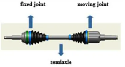
[image:2.612.204.415.431.545.2]

This manufacturing plant has 20 production cells, however, only 17 are scheduled to work according to customer’s needs. 357 different CVJ models are produced and each cell assemblies several models depending from the customer. To have all parts of each CVJ is required in order each cell can operate. Basically a CVJ is composed of three parts, as seen on Fig. 1, fixed joint, semi axle and moving joint. In general, the components can be classified in machining and miscellaneous. The machining components are the semi axle, inner race (in fixed joint) and boot (in moving joint). The miscellaneous ones are big clamp, small clamp, lock, cage, insert, etc. that are located as well in the fixed joint as in the moving joint. There is another important material not part of the CVJ signature, but which serves to protect the finished product called plastic.

Fig. 1. CV Joint components.

To If for any reason there is lack of any of the previously materials, the production cell stops and time elapses without operation (wait), which is called “losses due to lack of supply” and is measured since the production cell finished the model change (MC) until the forklift drivers (routers) deliver all parts required to assemble the CVJ of the scheduled model.

(3)

Due to the nature of the materials and design of vehicles, each router can transport in a single trip just one material, in other words, if the router is scheduled to carry machining to cell one and then to carry plastics to cell two, then the router must perform two trips.

It is assumed that the customer orders data and cells data where the different CVJ models will be manufactured are known and that they are recorded in each cell’s Heijunka box. The time required to process a lot of certain model depends on the quantity requested by the customer.

As the model change times are known, as well as the time associated with the scheduled orders, it is proposed to schedule the material’ s supplies in the temporary windows given by the duration of model change with the aim to keep at minimum the work in process time and also reduce the losses due to lack of supply.

In an ideal scenario, the purpose of the cell is only to produce and make model changes, according to the sequence scheduled and recorded in the Heijunka box. As noted in Fig. 2, where TPkl is the time required to process a lot of certain size, of model k

in cell 1 and TCDMl is the time required to prepare the machines so they can be able to produce the following scheduled k

model.

TPkl TCDMl TPkl TCDMl TPkl TCDMl

Fig. 2. Sequence in production cell.

In the case there is a delay in the deliveries of materials once the model change is completed, the production cell status will be waiting due to lack of supply and the production will be stopped until the delivery of required materials for the scheduled model is completed and therefore the final time to fulfill with all the orders will increase.

There are ideal periods of time at which the production of each model must be started, however, these can be affected due delays in materials supply.

There is only a limited number of vehicles, and the accomplishment of a model change can coincide in more than one production cell, there can occur that there is not enough capacity to give service to all cells simultaneously. Due to this, the aim of this work is to minimize the times that affect cells when materials are not completely supplied within temporary window due model change.

3 Problem description

Consider the problem of finding the optimum sequence for delivering required materials for assembly n lots of different products in L production cells and recorded in the Heijunka box. There is certain amount of limited resources for delivering materials known as routers or forklift drivers. Every material’s delivery is associated to a temporary window given by TCDMl

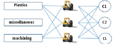
during which materials must be delivered with the purpose to start production of the following model scheduled in the cell at the ideal time, being this when the model change is completed. The system architecture is shown on Fig. 3.

Fig. 3. System architecture of delivery of materials.

The figure suggests that 3 routers can take materials from any warehouse (plastics and machining) and can deliver to any cell. The moment to deliver materials will be triggered by the finishing of a lot of certain model and the beginning of the model change time that is the already mentioned temporary window.

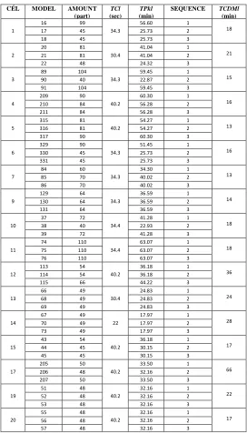
[image:3.612.214.398.549.620.2]

(4)

[image:4.612.170.442.129.606.2]

The company has a production schedule to fulfill, defined in a Heijunka box, where is found the model, the quantities to produce of each model and the sequence at which must be produced as listed on Table 1.

Table 1. Heijunka box for each cell

In column one is noted cell number, column two lists the model number to be produced, column three the amount of CVJ to produce, column four is the cycle time of the cell, column five represents the quantity to produce times cycle time (TPkl, in minutes), defining the time the cell will take to process the lot, in column six is found the sequence at which will be processed each model and in the column seven is the model change time.

The models part numbers of the joint have been recoded, assigning values from model 1 through 357. For example, cell 4 produces models from 209 to 314; cell 1 produces models 16, 17, 18, 19, 71, 72, 79, 80, 82, 83, 153, 155, 159, 161, 163, 165 and 167. Each production cell produces different CVJ models depending on the customer. All models were recoded without

CÉL MODEL AMOUNT (part)

TCl

(sec)

TPkl

(min)

SEQUENCE TCDMl

(min)

1

16 99

34.3

56.60 1

18 17 45 25.73 2

18 45 25.73 3

2

20 81

30.4

41.04 1

21 21 81 41.04 2

22 48 24.32 3

3

89 104

34.3

59.45 1

15 90 40 22.87 2

91 104 59.45 3

4

209 90

40.2

60.30 1

16 210 84 56.28 2

211 84 56.28 3

5

315 81

40.2

54.27 1

13 316 81 54.27 2

317 90 60.30 3

6

329 90

34.3

51.45 1

16 330 45 25.73 2

331 45 25.73 3

7

84 60

34.3

34.30 1

13 85 70 40.02 2

86 70 40.02 3

9

129 64

34.3

36.59 1

14 130 64 36.59 2

131 64 36.59 3

10

37 72

34.4

41.28 1

18 38 40 22.93 2

39 72 41.28 3

11

74 110

34.4

63.07 1

18 75 110 63.07 2

76 110 63.07 3

12

113 54

40.2

36.18 1

36 114 54 36.18 2

115 66 44.22 3

13

66 49

30.4

24.83 1

24 68 49 24.83 2

69 49 24.83 3

14

67 49

22

17.97 1

28 70 49 17.97 2

73 49 17.97 3

15

43 54

40.2

36.18 1

17 44 45 30.15 2

45 45 30.15 3

17

205 50

40.2

33.50 1

66 206 48 32.16 2

207 50 33.50 3

19

51 48

40.2

32.16 1

22 52 48 32.16 2

53 48 32.16 3

20

55 48

40.2

32.16 1

17 56 48 32.16 2

(5)

altering the information provided by the company, simply the part number the company used was changed by a consecutive number for this research project. This means there are 357 models of different CVJ’s and each one has its own part number.

The filling of each Heijunka box depends on the needs of the customers, and they are recorded in the company area known as supply chain.

The materials previously mentioned such as plastics and machining are delivered by 3 routers, which were assigned numbers from 1 to 3 (j = 1, 2 and 3) for their identification. Also the numbers 1 and 2 were defined to the warehouses, where plastic warehouse is 1 and machining warehouse is 2 (i =1, 2).

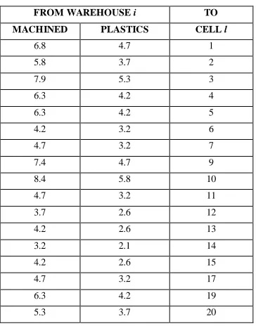
[image:5.612.216.398.233.465.2]

The average times at which the routers take the materials from warehouse i and take them to cell number 1, are listed in Table 2. This time is identified with STil, where STil it means Supply Time from warehouse i to the cell number l.

Table 2. Delivery times in minutes from each warehouse to every cell

FROM WAREHOUSE i TO MACHINED PLASTICS CELL l

6.8 4.7 1

5.8 3.7 2

7.9 5.3 3

6.3 4.2 4

6.3 4.2 5

4.2 3.2 6

4.7 3.2 7

7.4 4.7 9

8.4 5.8 10

4.7 3.2 11

3.7 2.6 12

4.2 2.6 13

3.2 2.1 14

4.2 2.6 15

4.7 3.2 17

6.3 4.2 19

5.3 3.7 20

In the current supply system, the routers are not aware about the sequence at which they must perform the delivery of materials, they have no knowledge of the materials they must supply, neither the quantities, nor the cell to which nor the time at which they must be delivered.

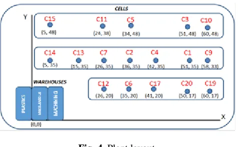
They use radio communication devices, where they are informed that there is need of material and must be delivered to a certain cell. This is not the best system to work, since there have been losses due to lack of supply in the order of 8% in average, to far from the company standards and it is affecting the equipment OEE in global, since the defined goal is that 1.5% is the maximum allowed.

(6)

Fig. 4. Plant layout.

Taking all the previously mentioned into account, the problem is defined as follows: given a production schedule, recorded in the Heijunka box of each cell, define the order at which the routers j = 1, 2, 3 will take the materials from the plastics and machining warehouses i = 1, 2 and they will deliver them to production cells l = 1,2,…, 20, in order to produce the k CVJ model

k = 1, 2, …, 357, fulfilling the production sequence in the Heijunka box and considering the restrictions of model change with the purpose to minimize the losses due to lack of supply.

4 Model of mixed-integer linear programming for losses due to lack of supply

The model herein described, is not found developed in specialized literature, is a novel model that defines the challenging situation for the particular case of the company. However, it can be used to represent similar situations in other companies, that work under lean manufacturing principles and have similar characteristics to the company herein analyzed: that can have a warehouse, routers to deliver materials and frequent model changes in their production cells. There were found only three studies with similar characteristics, in the first one there are orders and the production and distribution are coordinated to send products immediately to the customer considering a temporary window for its delivery, however in that paper it was found to maximize what they called the benefit associated to orders planning, with the aim the orders were delivered in the exact moment the customer requires them [13]. The second study was performed by Hung, proposing a heuristic approach for the solution of PEM where it was analyzed the production planning involving multiple products, multiple resources, multiple periods, model change times and costs [12]. The third was performed by Chiu, who proposed to solve a problem with multi deliveries to manufacture L products in a single machine using an algebraic approach in order to reduce de inventory his model is called multi item economy production quantity (EPQ) [14].

In the problem described herein, if Xijkl is the decision variable, the subindex i defines the warehouse number, the subindex j

means the router, the subindex k means the CVJ model and the subindex 1 means the production cell. The variable Xijkl is of binary type, whose values are defined below.

The variable Tjk is defined as the time that is lost before starting with model k, this means the wait due to lack of supply before starting the model k production.

The variable Xk defines the time at which the cell starts the production of model k lot.

The variable TPkl, represents the time required to produce the lot of model k, in cell 1. The time defined in this variable depends on the lot size of model k to be produced.

[image:6.612.188.426.69.216.2]

(7)

(1)

Subject to:

𝑇𝐶𝐷𝑀𝑙 = 𝑇𝐶𝐷𝑀 𝑜𝑓 𝑡ℎ𝑒 𝑝𝑟𝑜𝑔𝑟𝑎𝑚𝑚𝑒𝑑 𝑐𝑒𝑙𝑙𝑠 (2) 𝑋𝑘 = 0 𝐹𝑜𝑟 𝑡ℎ𝑒 𝑓𝑖𝑟𝑠𝑡 𝑚𝑜𝑑𝑒𝑙𝑠 𝑠𝑐ℎ𝑒𝑑𝑢𝑙𝑒𝑑 (3)

𝑇𝑃𝑘𝑙 = 𝑆𝑐ℎ𝑒𝑑𝑢𝑙𝑒𝑑 𝑚𝑜𝑑𝑒𝑙 𝑛𝑢𝑚𝑒𝑟 𝑘 𝑚𝑢𝑙𝑡𝑖𝑝𝑙𝑒𝑑 𝑏𝑦 𝑡ℎ𝑒 𝑐𝑦𝑐𝑙𝑒 𝑡𝑖𝑚𝑒 𝑜𝑓 𝑡ℎ𝑒 𝑐𝑒𝑙𝑙 𝑙 (4)

𝑋𝑘 = 𝑇𝑃𝑘−1,𝑙 + 𝑇𝐶𝐷𝑀𝑙 + 𝑇1,𝑘 ´ + 𝑇2,𝑘 ´ + 𝑇3,𝑘 ´ 𝑓𝑜𝑟 𝑎𝑙𝑙 𝑘 𝑚𝑜𝑑𝑒𝑙𝑠 𝑠𝑐ℎ𝑒𝑑𝑢𝑙𝑒𝑑 𝑖𝑛 𝑠𝑒𝑐𝑜𝑛𝑑 𝑎𝑛𝑑 𝑡ℎ𝑖𝑟𝑑 𝑝𝑙𝑎𝑐𝑒 (5)

Deviation from the ideal time to supply materials k =1, 2, …, 357 (according to the heijunka)

𝑇1,𝑘´ − 𝑇1,𝑘´´ = 𝑆𝑇1𝑙𝑋1,1,𝑘,𝑙 + 𝑆𝑇2𝑙𝑋2,1,𝑘,𝑙 (6) 𝑇2,𝑘´ − 𝑇2,𝑘´´ = 𝑆𝑇1𝑙𝑋1,2,𝑘,𝑙 + 𝑆𝑇2𝑙𝑋2,2,𝑘,𝑙 (7) 𝑇3,𝑘´ − 𝑇3,𝑘´´ = 𝑆𝑇1𝑙𝑋1,3,𝑘,𝑙 + 𝑆𝑇2𝑙𝑋2,3,𝑘,𝑙 (8)

Securing the supply of plastic and machined for each model programmed in heijunka

𝑋1,1,𝑘,𝑙 + 𝑋1,2,𝑘,𝑙 + 𝑋1,3,𝑘,𝑙 = 1 (9)

𝑋2,1,𝑘,𝑙 + 𝑋2,2,𝑘,𝑙 + 𝑋2,3,𝑘,𝑙 = 1 (10)

𝑋𝑖𝑗𝑘𝑙 ∈ {0,1}, 𝑇𝐶𝐷𝑀𝑙, 𝑋𝑘 , 𝑇𝑃𝑘𝑙 ≥ 0, 𝑇𝑗𝑘 𝑢𝑛𝑟𝑒𝑠𝑡𝑟𝑖𝑐𝑡𝑒𝑑

The objective function seeks to minimize the percentage of losses due to lack of supply when router j = 1,2 or 3 supply materials in order to produce the model k (see equation 1). The equation (2) is the restriction that allows updating the times of model change, since in a lean production system the trend is to reduce the model change duration, as a continuous improvement process. The equation (3) is the restriction that indicates the start time of production of the first scheduled model in the Heijunka box is the minute zero. This is to assume that the system works in stable conditions, where all cells already have materials to start their operation. The equation (4) defined the required time (in minutes) to complete each one of the lots of k models, scheduled in cell 1. The equation (5) represents the start times of each scheduled model in the second and third place of each cell. The equations (6 to 8) are defined with the support of unrestricted variables (Tjk = Tjk´ – Tjk´´) due to the materials supply made by router j can exceed the model change time (TCDMl), in this case Tjk will have a positive value, which indicates that there are losses due lack of supply. On the other hand, if the materials supply is made in a time shorter than TCDM1, the Tjk

value will be negative. For the purpose herein, the values that we look to reduce are the positive Tjk, which are seen in the function. The equations (9 and 10) guarantee that plastic and machining are delivered to the cells.

5 Results analysis

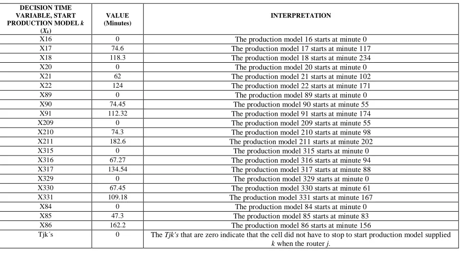
It was considered the production schedule shown in the Heijunka box of Table 1 in section 3, for building the model, then solving it by branch and bound method, explained in the previously section and with help of Win QSB software there are obtained the results listed below.

(8)

[image:8.612.80.532.84.333.2]

Table 3. Part of the solution

DECISION TIME VARIABLE, START PRODUCTION MODEL k

(Xk)

VALUE (Minutes)

INTERPRETATION

X16 0 The production model 16 starts at minute 0

X17 74.6 The production model 17 starts at minute 117 X18 118.3 The production model 18 starts at minute 234

X90 74.45 The production model 90 starts at minute 55 X91 112.32 The production model 91 starts at minute 174 X209 0 The production model 209 starts at minute 55 X210 74.3 The production model 210 starts at minute 98 X211 182.6 The production model 211 starts at minute 202

Tjk´s 0 The Tjk's that are zero indicate that the cell did not have to stop to start production model supplied k when the router j.

[image:8.612.173.440.398.713.2]

Finally in the Table 4, we present the results of the variables Xijkl indicating the assignment of every router in order to supply materials and meet the production schedule.

Table 4. Part of the assignment of the routers

VARIABLE TO THE ROUTERS

(Xijkl)

VALUE INTERPRETATION

X1,2,17,1 1 Carrying plastics, router 2 to produce the model 17 in cell 1

X2,2,17,1 1 Carrying machining, router 2 to produce the model 17 in cell 1

X1,3,18,1 1 Carrying plastics, router 3, to produce the model 18, in cell 1 X2,3,18,1 1 Carrying machining, router 3, to produce the model 18, in cell 1 X1,3,21,2 1 Carrying plastics, router 3, to produce the model 21, in cell 2 X2,3,21,2 1 Carrying machining, router 3, to produce the model 21, in cell 2 X1,3,22,2 1 Carrying plastics, router 3, to produce the model 22, in cell 2 X2,3,22,2 1 Carrying machining, router 3, to produce the model 22, in cell 2 X1,3,90,3 1 Carrying plastics, router 3, to produce the model 90, in cell 3 X2,3,90,3 1 Carrying machining, router 3, to produce the model 90, in cell 3 X1,3,91,3 1 Carrying plastics, router 3, to produce the model 91, in cell 3 X2,3,91,3 1 Carrying machining, router 3, to produce the model 91, in cell 3 X1,2,210,4 1 Carrying plastics, router 2, to produce the model 210, in cell 4 X2,2,210,4 1 Carrying machining, router 2, to produce the model 210, in cell 4 X1,3,211,4 1 Carrying plastics, router 3, to produce the model 211, in cell 4 X2,3,211,4 1 Carrying machining, router 3, to produce the model 211, in cell 4 X1,2,316,5 1 Carrying plastics, router 2, to produce the model 316, in cell 5 X2,2,316,5 1 Carrying machining, router 2, to produce the model 316, in cell 5 X1,3,317,5 1 Carrying plastics, router 3, to produce the model 317, in cell 5 X2,3,317,5 1 Carrying machining, router 3, to produce the model 317, in cell 5 X1,3,330,6 1 Carrying plastics, router 3, to produce the model 330, in cell 6 X2,3,330,6 1 Carrying machining, router 3, to produce the model 330, in cell 6 X1,3,331,6 1 Carrying plastics, router 3, to produce the model 331, in cell 6 X2,3,331,6 1 Carrying machining, router 3, to produce the model 331, in cell 6 X1,3,85,7 1 Carrying plastics, router 3, to produce the model 85, in cell 7 X2,3,85,7 1 Carrying machining, router 3, to produce the model 85, in cell 7 X1,3,86,7 1 Carrying plastics, router 3, to produce the model 86, in cell 7 X2,3,86,7 1 Carrying machining, router 3, to produce the model 86, in cell 7

Xijkl

different of 1 are equal

zero

0 Decision variables to assign routers, not basic

(9)

6 Conclusions

By the application of mixed-integer linear programming, it was achieved to reduce losses due to lack of supply from 8% down to 0%. It is possible that the goal the company proposes is not feasible, however to reduce from 8 to 0% significantly contributes to improve OEE giving the cell the opportunity to produce more quantities of CVJ’s. For instance, in a 7.5 hours shift, there are available 450 minutes. If losses due to lack of supply represents 8%, then 36 minutes or 2160 seconds are lost. Considering cell 1 has a CT=34.3 s, dividing 2160 between its CT, 62.97 is achieved, this means that in a shift that has 7.5 hours, 63 CVJ’s are ceased to be produced in cell 1. On the other hand, if the losses due to lack of supply are only 0%, and applying the same procedure, there are only 13.77 CVJ ceased to be produced.

With regards efficiency of branch and bound method, it is concluded that 3961 iterations were performed with a maximum amount of nodes of 24. The total execution time of the processing unit was of 261.047 seconds. Given the need to obtain results in short term to fulfill the company requests and to give answer to the customers, it is required the use of tools that allow to obtain quality solutions in a reasonable short time, like the metaheuristic algorithms. In the future, it is proposed to solve this same problem by the heuristic search and genetic algorithms, since they have demonstrated to give better results when applied to problems of the real life and manufacturing problems [15, 16].

Acknowledgment

The authors would like to the Concyteg due to the support for the project in the program “Joven Investigador 2015”. And as part of the National Research Network "Sistemas de Transporte y Logística”, the authors acknowledge all the support provided by the National Council of Science and Technology of Mexico (CONACYT) through the research program “Redes Temáticas de Investigación”. At the same time, we acknowledge the determination and effort performed by the Mexican Logistics and Supply Chain Association (AML) and the Mexican Institute of Transportation (IMT) for providing us an internationally recognized collaboration platform, the International Congress on Logistics and Supply Chain [CiLOG].

References

The list of references should only include works that are cited in the text and that have been published or accepted for publication. Personal communications and unpublished works should only be mentioned in the text. Do not use footnotes or endnotes as a substitute for a reference list.

1. Abdulmalek FA y Rajgopal J.: Analyzing de benefits of lean manufacturing and value stream mapping via simulation: a process sector case study. International Journal of production economics. Vol. 107. p.223-236. (2007) doi: 10.1016/j.ijpe.2006.09.009

2. Padilla L:. “Lean Manufacturing”. Revista Electrónica Ingeniería Primero. No.15. p.64-69. ISSN: 2076-3166 (2010)

3. Fullerton R.R., Kennedy F. A., Widener S.K.: Lean manufacturing and firm performance: The incremental contribution of lean management accounting practices. Journal of Operations Mangement. Vol. 32, 414 – 428 (2014)

4. Shah R y Ward PT.: Lean manufacturing: context, practice bundles and performance. Journal of operations management. Vol. 21 No. 2, p. 129-149. (2003) doi: http://dx.doi.org/10.1016/S0272-6963(02)00108-0

5. Cusumano MA.: The limits of lean. Solan Managgement Review. Vol. 35, No. 4. p. 27-32 (1994)

6. Jiménez-García JA, Medina-Flores JM, Yáñez-Mendiola J y et al.: Diagnostico en el surtimiento de materiales en líneas de ensamble de flechas de velocidad constante Utilizando Promodel. En: Actas del 1er Congreso Internacional de investigación e innovación 2012. Multidisciplinario, (26 y 27 de abril de 2012). ISBN: 978-607-95635

7. Jimenez J. A., Medina J. M.., Yáñez J., Mezura E. Waiting waste reduction in assembly lines using heuristics and simulation scenarios . DYNA, 89(1). 50-60. (2014) doi: http://dx.doi.org/10.6036/5833

8. Jiménez J. A., Telléz S., Medina J.M., Rodríguez H.H., Cuevas J.: Materials Supply System Analysis Under Simulation Scenarios in a Lean Manufacturing Environment. Journal of Applied Research and technology. Vol. 12, 829 – 838 (2014)

9. Ohlmann JW, Fray MJ, Thomas BW.: Route Design for Lean Production Systems. Transportation Science. Agosto 2008. Vol. 42. No.3. p.352-370. (2008) doi:10.1287/trsc.1070.0222

10. Grimard C, Marvel JH.: Validation of the re-design of a manufacturing Work cell using simulation. Proceedings of the 2005 Winter Simulation Conference. p.1836-1391. ISBN:0-7803-9519-0 (2005)

11. Bermudez-Colina Y.: Aplicaciones de programación lineal, entera y mixta. Ingeniería Industrial. Actualidad y nuevas tendencias. Año 4. Vol. 2. No. 7. 84 -104, (2011)

(10)

13. García J. M., Vila G., Calle M. y Andrade J.L.: Algoritmo de búsqueda Tabú para la planificación coordinada de la producción y distribución con ventanas temporales. Métodos cuantitativos en organización industrial. P. 733-740.

14. Chiu Y.S., Wu M. F., Chiu S.W., Chang H. H.: A simplified approach to the multi‑item economic production quantity model with scrap, rework, and multi‑delivery. Journal of Applied Research and Technology. Vol. 13, 472 – 476 (2015).

15. Dero J, Siarry P, Michalewickz Z y et al.: Metaheuristics for Hard Optimization, Springer, 2008. 372p. ISBN: 978-3-540-30966-6