Short term economic load allocation : a report

LOAD ALLOCATION

A Report presented for the degree of Master of Electrical Engineering

in the University of Canterbury Christchurch, ·New Zealand

by

M • D • T u r n e r , B • E • ( H.o n s , )

ABSTRACT

The method of equal incremental cost of received power is well established as a means

or

determining the most economic distribution of active power, while

satisfyin~ the power system load demand, subject to

generation and water constraints,

ACKNOWLEDGMENTS

I wish to thank my supervisor, Mr W.H. Bowen, for his interest and encouragement, and the other members of the Electrical Engineering Department staff who assisted during this project.

CONTENTS

Page No.

Title Page i.

Abstract ii.

Acknowledgments iii.

List of Contents iv.

SECTION ·1 INTRODUCTION 1 • 1

1. 2 1.3

1.4

Optimal Operation of a Power System Economic Load Scheduling Techniques Requirements of Load Allocation methods Economics of Computer Calculation

1

4

6 7

SECTION 2 THE CONCEPTS OF SHORT TERm OPTimIZATION

2 .1 Development of Co-ordination Equations

2.2 Transmission Losses

2.3 methods of Solving the Co-ordination Equations

2.4 Load Demand Variation

2.5 Derivation of Incremental Plant Cost 2.6 Complete Solution of the Co-ordination

2.7

2.8

Equations

Calculation of Base Case Schedule Summary

9

14

19

23 23

28

32

SECTION 3 DIGITAL COMPUTER PROGRAM LANZOP 3 .1

3,2 3,3

3.4

3.5

3.6

3,7

3·, 8 3,9

Introduction

The System Model

Transmission Losses

Implementation of the Co-ordination Equations

Calculation of th~ Generation Schedule

Spinning Reserve

Performance of the Program

Schedule Diagnostics

Summary

Page No.

38 39

41

41

44

66 66

68

68

SECTION 4 RESULTS, CONCLUSIONS AND RECOMMENDATIONS

4 .1 Accl!racy of the Schedule 69

4.2 Schedule Output 74

4.3 Evaluation of Savings 77

4.4 Alternative Methods for Economic Scheduling 85

4.5 Conclusions 86

4.6 Recommendations 88

REFERENCES

APPENDIX A

APPENDIX B

90

PROGRAM LISTING AND SELECTED SYMBOL LIST

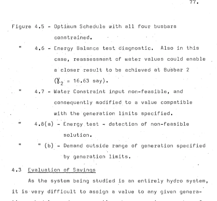
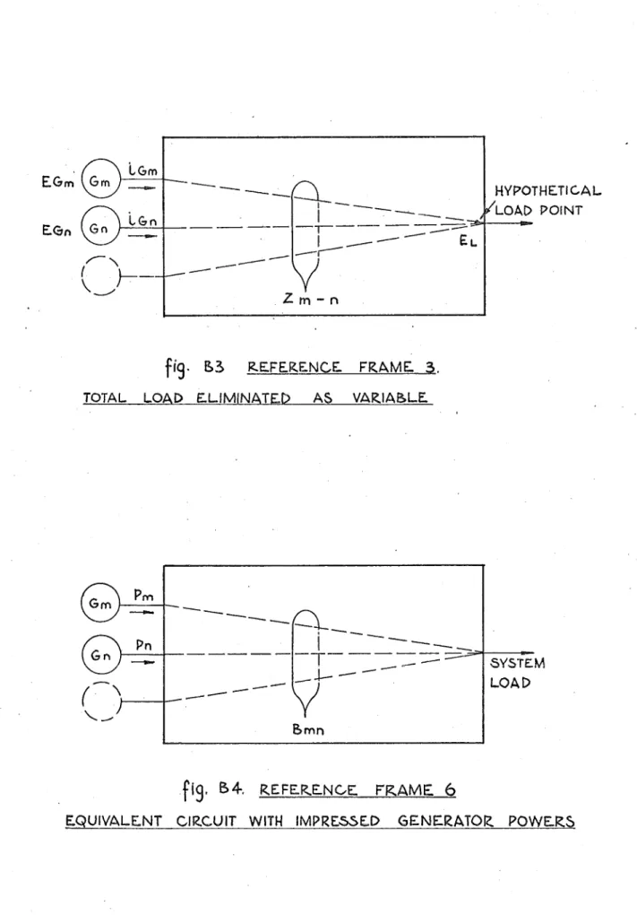
AN OUTLINE OF THE DERIVATION OF THE LOSS

INTRODUCTION

1.1 Optimal Operation of a Power System

This report considers the optimal operation of a power system from an economic point of view, The aim of economic operation is to meet the system load demand as it varies over a given time period, at the minimum total cost while complying with the phys~cal limits imposed by the system,

With the advent of large high-speed computers it is now possible to consider load scheduling (i~e., the

distribution of generation to meet the load) in much

greater detail and to determine the schedule of available generation in a large system, much more accurately than possible previously,

The optimal operation of an integrated power system (both hydro-electric and thermal generation in the system) is a complex task as each type of generation has its own peculiar characteristics and limitations, This complexity makes it necessary to divide the overall system problem into a number of subproblems which can be considered independently, even though the subproblems are in fact interconnected and not totally independent. Economic

security, system planning. Ther~ are a number of ways in which this division may be made, on~ of the most usual being undertaken on a time basis.

This permits divisi?n into two main streams -(i). Long term operation

(ii) Short term operation 1.1.1 Long Term Operation:

The long term operation of a power system may be

further div"ided into two time periods, namely, the planning period, and the operational co~trol period. In this report, long term operation will refer to the operational control period, which may be considered to range from one week to

'

three years, while the planning time period may range

upward of three years and is principally concerned with the "why, when and where" of the installation of equipment in the system.

The long term operation, then, in an integrated system is concerned with the allocation of energy resources to ensure continuity of supply, at a minimum cost. In order to achieve these objectives, the use of the water and the thermal resources must be coordinated so that at any time -(a) the thermal costs are not made excessive by an

endeavour to preserve a more than adequate reserve of water for later use in the system, or,

The decision on the distribution of generation betwe~n

the two basic resources is the important long term decision, but the results of this must be reflected in the short term operation of the system.

1.1.2 Short Term Operation:

The short term operation is concerned with daily or weekly operation of the system subdivided into suitable time intervals. The available generation, system mainten-ance requirements, and the constraints imposed by transmission limitations must be considered during these time intervals, and the water allocatibn for the time period should be

achieved, The aim cif economic allocation in the short term is to minimise the total cost subject to the above constraints while ensuring satisfaction of the load demand.

The following cost factors are significant in con~idering

the total cost of a power

system:-(i)

(ii) (iii) (iv)

(v)

New capital works

The servicing of loan moneys and depreciation Administrative costs

Maintenance and labour fuel for thermal plant

The first four costs can be considered as fixed costs in the short term, and consequently the only variable cost in the short term which is directly applicable to the

operation become~ the minimisation of the cost of thermal generation, (There .are other less significant costs, which if they can be related directly to the system

generation, such as gas turbine maintenance, may be added as a small cost component to the total fuel cost •. )

The long term optimization results in water constraints (water allocation) which must be considered in the short term, and generally the water to be used in a given catchment or

pla~t

is. then defined for the short term1• The value or cost of water may then be indirectly related to the storage requirements in the water reservoirs, and the most probable replacement value of the equivalent generation from thermal plant. The assignment of a value to the water in each catchment or hydro-electric plant is necessary to enable the calculation of the optimum economic generation schedule to be made.

1.2 Economic Load Scheduling Techniques

The classical load dispatching methods deal with the economic allocation of active generation only. These methods may or may not include the system transmission losses depending upon the significance of these losses in the system being modelled.

being made that the network is capable of distributing the power as scheduled satisfactorily in all cases. This assumption is often too generalis~d and methods are being developed to overcome this weakness of the classical methods, The only constraints normally considered in each time

interval, when scheduling active pbwer are the maximum and minimum generation limits.

The classical methods may be divided into two main categories, that of "merit order"· scheduling, and that

of "equal incremental cost" scheduling. The "merit order"

2

method is used principally in large thermal systems such as that of the British Cent~al Electricity Generation Board, and is based on the cost of generation at each station derived from the thermal ~erformance of the plant and the cost of

the fuel supplied to that station. The generation is dispatched so that the overall cost of generation is minimised with due regard to the security of supplyo This means that the large and most modern stations with

the lowest incremental cost are scheduled first as base load stations, with the next least expensive stations being loaded sequentially until the load demand is satisfied. This method does not involve significant hour to hour computation and is easily carried out.

operating at the same incremental cost within their operating capacity.

These methods involve a large amount of computation even for a relatively simple system and hence the

development of incremental cost slide rules and with the . advent of computers, prQgrams for th~ complex calculations.

(The "merit order" method may be considered as a simple form of the "equal incremental cost" method, as the merit .order is established by the incremental cost of the plant,

the incremental cost characteristic being constant and independent of the outputo)

For an integrated system, where there is significant hydro generation, the "'merit order"' approach is not

particularly practical, as the·overriding constraints in a hydro system are the water allocation constraints which are predetermined from the long term considerations,

Hence the development of the "equal incremental cost" method for integrated power systems and the purpose of this report is to discuss the theory behind the method and its application to the New Zealand Power System, 1,3 Reguirements of Load Allocation methods

An y me th o d use d f o r 1 o ad a 11 o.c at i on s ch e du 1 in g should meet the following

requirements:-(i) Simple to use

(ii) minimum input information required

(iv) Easily interpreted results

With the increase in system complexity, manual methods no longer meet these requirements, but with the availability of high speed digital and analogue computers, complex

systems may now be handled, and the above requirements satisfied. Both analogu~ and digital.methods have been developed, but in this report only the implementation on a digital computer has been considered. The analogue computer has a significant role to play in on-line applications of syst'em control, particularly .for inter-area economic

allocation as developed by a number of Electric Power Supply utilities in the U.S.A. The chief disadvantages of analogue computers are their high cost and relatively specialised use, which may be justified for their automatic control applications and high speed operation in a large system.

1.4 Economics of Computer Calculation

The implementation of a suitable method by computer

may result in significant savings in power station operation. Electric power generat~on represents a significant factor in the national economy. Effective utilisation of the resources available reduces the exp~nditure of capital on equipment, and realizes the maximum capability of the resources. A small error in .the co-ordination of these resources therefore, can cause unnecessary expenditure. Computer based calculations

-(i) Reduce casts by:

(b) including factors (e.g., transmission losses) which are usually omitted in manwal methods. (ii) Reduces the manpower required and allows the

realignment of this manpower to other duties. The savings possible.above are offset by the·high annual .cost of computer operation~ and the use of the

computer and its facilities may need optimizing to prevent excessive computing time for marginal gain in savings.

SECTION 2

THE CONCEPTS OF SHORT TERm OPTimIZATION

2.1 Development of Co-ordination Equations

The problem of short term optimization for a combined hydro-thermal (integrated) power system is that of minimising the total input into the system while satisfying the current load demand and the constraints imposed by the system itself and the constraints imposed by management,

In allocating the generation tha ov~rriding constraint which must be met is that of the system load demand. (As discussed in Section 1, the discussion will be limited to that of real (active) power allocation,)

where

This may be represented thus

-n

i

p,

l

P.

l

=

the power

p d

R

=

0

output of Plant i (mW) PL

=

the system transmission losses (mw)

n d _the

system load demC1nd (r11W)

r-R

=

n

₌

the number of power plants (both thermal and hydro)

In an integrated power system, the total input cost can be considered as the total fuel cost for the thermal stations.

Hence _

where CC

i

and F.

l

=

=

= = =

total cost ($/hr)

oC

2: F.

l

i=1

the number of thermal stat io.ns 1 , e I • I I I I

.ex.

the fuel cost for plant i ($/hr)

The short term optimization requires that

-/ t

Ft dt =

to

minimum

where t-t₀ = the fixed time period defining the short time interval

Since the time period is broken up into discrete time intervals, the object is to minimise

-t <X.

t i=1

0

F.

l

In addition to the demand constraint applying for each interval, the long term water resource allocation will

impose water constraints on the sys~em. Therefore the total input cost must be minimised subject to the water constraints

-t

t 0

w.

~t

where W.

J

=

the turbine discharge of hydro plant j (cusses)

=

W. (P .) a function of the generation from

J J

plant j

K.

J water allocated for plant j

As stated in Section 1, one criterion which can be used to achieve optimum scheduling is for all generation sources to be operated at equal incremental cost. This concept can be ~rrived at intuitively. Assume that all generation

sdurces are not operating at the same incremental cost. Consequently some sources would be operating at a higher inqremental cost than others. It would then be possible to reduce the system input by decreasing the generation on the higher cost source and increasing the generation on the lower cost source.· In the limit, all .sources should be operated at the same incremental cost. This is expressed in the· statement of the SO=called Co-ordination Equations:

dF. _~PL

l

A

/\

for thermal plant

dP. + oP. =

l l

dW. _cPL

~·

_ J ₊

"A

=

I\

for hydro plant

J _dP. oP.

J J

that is, the minimum input cost for a given system load demand is obtained when the incremen~al cost of generation at a given plant plus the cost of the incremental trans-mission losses associated with that generation charged at the system incremental cost is the same for all gensration plant.

( 2 )

Consider equation (2) for the the rm al plant 3 Let F.

l

=

input to plant .i ($/hr)

Ft

=

total input to the ·system ($/hr) then Ft

=

~F. l

let PL

=

total transmission losses ( fYlW) and _PR d

₌

system load demand

₌

_{PR ( fYlW)}

PR

=

received power ( fYlW)

To achieve the. optimum allocation, it is necessary to minimise total input Ft

-let F

₌

_Ft

_f\\jl

applying the method of Lagrange multipliers where

A

=

Lagrange multiplier,

The constraining relationship is given by

-=

0

fYlinimum input for a given load is obtained when

-oF

₀

~P.

=

l

then _oP. ~F

₌

~Ft

/\

~

₌

0

oP. oP.

l l l

oFt ₀

(~ _PR)

I •

oP.

·-

'A

oP. P. l PL

=

0

l l

i and hence ()Ft

oP. +

:A~

oP.

=

'A

~

oF

t

o

(2F i)

o

F. dF.

Ft

P.

1 1

now

₌

_{i • •}

w.

₌

_a

_P.

₌

_oP.

₌

_@.

1

1 1 1 1

dF. _~PL

1

x

then _dP. +

_A

_oP.

=

1 1

The thermal plant co-ordination equation where

-dF.

1

dPL

=

=

=

incremental plant cost at plant i ($/mWh)

incremental transmission losses associated with plant i (mw/mw)

incremental cost of received power ($/mWh) The incremental transmission losses are costed by charging them at the incremental cost of received power.

In a similar manner4 the co-ordination equations (2)

and (3) can be derived for an integr~ted power system from the equation of constraint

-t1

subject to

2:

w. .D. t

₌

K.

J J

t

0

where ~P.

₌

l total thermal generation (mw)

::g

p j

₌

total hydro generation (mw) w. t:!

J water flow from plant j (cusses)

K.

₌

allocated water (cu.ft)

J

t

₌

_t1

-

t

₌

optimization period

0

t1

and as before _{~ Ft} At

₌

minimum is required t

Then the co-ordination equations (2) and ( 3) are

-dF. _dPL

1

dP. +

I\

~p.

=

1 1

dW. . oP

~· _ J + L

A

A

dP.

=

J dP.

where ..:.:.:..:..J. dW. dP.

J

'K .

J J

=

=

J.

incremental water rate of hydro plant j

(cusecs/mw)

cost of water ($/(cu.ft x 106) say)

and then dW · J

₌

incremental plant cost of hydro plant j @.

J

The ~j constants are the set of Lagrange multipliers chosen so that the allocated amount of water is used by

each hydro plant, and is effectively a conversion coefficient which converts incremental water rate to incremental plant cost, The derivation assumes that during the given time period, the operating head of each hydro station is constant, and this is implied in the constant conversion coefficient

~•I J

2,2 Transmission Losses

The co-ordination equations derived include the effect of the system transmission losses.

~.

J

Without these losses the equations reduce to -dF.

1

-

_dP.

='A

1

dW. __J_

dP.

J.

that is; all plant operates at the same incremental plant cost which is equal to the system incremental cost of

received power.

The system transmission los~es need to be considered in order to achieve optimum economy since ignoring these losses does not penalise gener~tion plant which may have significant transmission losses associated with it5•

Kirchmayer and Stagg in reference 5 have shown.that including the incremental transmission losses substantially reduces the fuel cost,

2,2,1 Evaluation of Trahsmission Losses:

The evaluation of the transmission losses and the corresponding incremental trans~ission losses has been

greatly facilitated by the development of transmission loss formula expressing the losses in terms of generator power (the source powers). The loss formula allows the losses to be calculated quickly and accurately, Rapid calculation of losses must be possible in any method of co-ordination because of the large number of times they are evaluated during the production of an economic load schedule, when scheduling on the basis of received power equal to demand.

The loss formula in its full form is

-~ _m p B p + ~ 8 p + 8

m mn n n no n oo

where ~ is summation of powers P

n

8 are the derived transmission loss

00

formula coefficients

The full expanded form of the loss formula allows

( 4 )

involved in deriving the coefficients need to be less rigidly adhered to over a range of operating conditions, It has been shown by Kirchmayer et al,6 that the additional savings obtained by using the 16ss formula with the linear and constant terms are marginal, for a system of reasonable complexity, and for the purposes of this report the trans-mission losses will be evaluated using the standard

Quadratic formo

=

p B p

=

total transmission

m mn n _{losses (5)}

where B _mn

=

p

n =

loss formula coefficients (a symmetrical n x m matrix)

generation of plant n

number of generation plant

For a brief treatment of the derivation of the trans-mission loss formula and the B coefficients refer to Appendix

B.

are

-From equation (5), the incremental transmission losses

d P,

L

6Pn =

=

d

w

_n

2

2:

n

(2.:

m

B p

mn n (6)

This .form of the incremental transmission losses is very suitable for incorporation into the co-ordination equation as it involves only straight forward matrix

The co-ordination equations can now be written including the losses,

dF.

2;

l

/\ (2 B p )

_'A

( 7)

~ + i mn n =

l

and _{~· _ J} dW. +

A

(2 ~ B p ) =

I\

( 8)

J j mn .n

dP. J

where m, n = total number of generation plant

In full, differentiating between hydro and thermal plant

-dF.

(~

?>

l

2A

B. _Psm

2:

B. _PHn)

_A

dP. + im + n=CX::+1 in =

l m=1

(7a)

dW.

_f>

oc

~

--

J + 2 i\ ( _~ B. _{PH n} + _~ B. _Psm) =

A

j dP. _{n =OC+ 1} Jn _m=1 Jm J

(Ba)

where i = thermal plant number i=1 , I I t o o< m = thermal plant number m=1, I I I

,ex

j _{= hydro plant number j =<X+ 1 ,} •••• J!>

·P

n = hydro plant numbs r n =o<'.+ 1 , I t I I

Ji

C( ₌ total number of the rm al plant

J3 = total number of generation plant

/3

-<X = total number of hydro plant

Since the losses are calculated using the loss

coefficients~-(i)

The equivaleFlt load current at any busbar remains a constant complex·fraction of the total equivalent load, The equivalent load current at the busbar is defined as the sum of the line charging, synchronous condenser, and load currents at that bus.

(ii) The generator bus voltage mag~itudes and angles remain constant.

(iii)

The ratio of reactive power to real power of any

generation source remains constant.

These assumptions are necessary to allow the expression of ·the transmission losses in terms of generator powers only.

There is an alternative method of calculating the losses, in a form suitable for.use in the co-ordination

7

equations, based on the-work of Brownlee considering the losses as functions of the voltage phase angle. However, Kirchmayer has shown that in gener~l, this method is less accurate than the B coefficient method in a system of reasonable complexity. This method has not been used extensively in power system operation and will not be discussed further.

The B coefficient loss formula describes the system losses in terms of generated power only, and therefore the

system configuration from which they were derived is submerged, This fact and the need for the assumptions made, lead to a

number of weaknesses in the method and hence in the results of the solution of the co-ordination equationso The

-(i) The system network must be of such a form so as to enable the satisfying of the assumptions used in the B coefficient derivation,

(ii) A solution may be obtained which is not physically .realizable because of the limitations of voltage,

active and reactive power, inherent in the system, as the B coefficients once derived do not take any limits i.nto account.

(iii) Stability limits may be exceeded and an unstable power allocation scheduled,

(iv) No optimization of the reactive power component is considered, and hence a true power optimum is not obtained,

2,3 methods of Solving the Co-ordination Equations Consider equation (2)

-+ =

as representative of all forms of the co-ordination equations. It is a non-linear equation in

A

since the incremental

transmission losses are charged at

incremental cost of received power

(A).

There are three basic methods used in solving these equations

-(i) Exact solution of the non-linear simultaneous equations (ii) Approximate solution by using linear simultaneous

equations

2,3,1 The Non-linear Equations:

The non-linear equations must be solved iteratively for the power generation, since the value of

A

is not known which satisfies the load demand, Within this iterative procedure, an inner iteration is required to calculate the losses and hence the generation since the losses are unknown until the power distribution is known. 2.3.2 The Approximate Solution:

If the incremental transmission losses are charged at a constant rate ~ which closely approximates

A

then the resulting equations are linear,

df

n

dPn +

=

( 9)'

where ~ can be considered as the average cost of received power, Rewri:ting the

df n

a

PL

(jjJ +

w

n n

above equation

-"A

=

fJ

=

if ~

=

1 then the equations correspond to the exact non-linear equations,

2,3,3 The Penalty Factor method:

The penalty factor method charges the incremental transmission losses at a rate corresponding to the

(9a)

incremental plant cost, when using the approximate penalty factor

L

_n

From equation (2)

-dF

n

[jp

the penalty factor Ln is defined as 1

=

for plant n

then

the solution of which is identical to that of the exact solution. This exact penalty factor is usually

approximated by

-Ln'

=

approximate penalty factor . oPL

= ( 1 + w ) . n

and co-ordination equation becomes:

dF n

dP

n

L

I

n

=

The results are a close approximation to the exact solution oPL

since (1 - oPn) ~ 1.

2,3,4 Evaluation of methods:

Kirchmayer and Stagg (reference 5) have evaluated these three methods cif co-ordinating the incremental

plant costs and incremental transmission costs in detail. They conclude after study and their application to the American Gas and Electric Company's system

of the .exact non-linear equations.

(ii) For large integrated systems, savings of considerable magnitude can be realized when the effects of the transmission losses are included in the economic ·schedule of generation.

Chandler, Dandeno et al. 8 also considered three alternative methods, and applied them to the Ontario Hydro integrated system •

. (i) Exact solution of co-ordination equations (ii) Equal incremental plant ~osts (i,e;, ignoring

transmission losses)

(iii) Maximum efficiency operation of hydro plant, with thermal plant scheduled by

-(a) Equal increm~ntal fuel cost (b) Exact co-ordination equations

The results of this study showed clearly the

superiority of the co-ordination equations (with transmis-sion losses) over the other methods considered.

Therefore the two approaches, the exact and approximate solution of the non-linear co-ordination equations are

those best suited for economic scheduling. However, in. using the approximate solution, (i.e., equation 9)

-dF

n

dP

_n +

=

operating with minimum transmission losses, which is not that of minimum cost. Therefore care must be taken in choosing a value of fo so that the linear solution is a close approximation to.the exact solution. This may mean considerable work itself and in this report, the exact solution of the co-ordination equations has been applied, in gaining experience with the methods, to the New Zealand Power System.

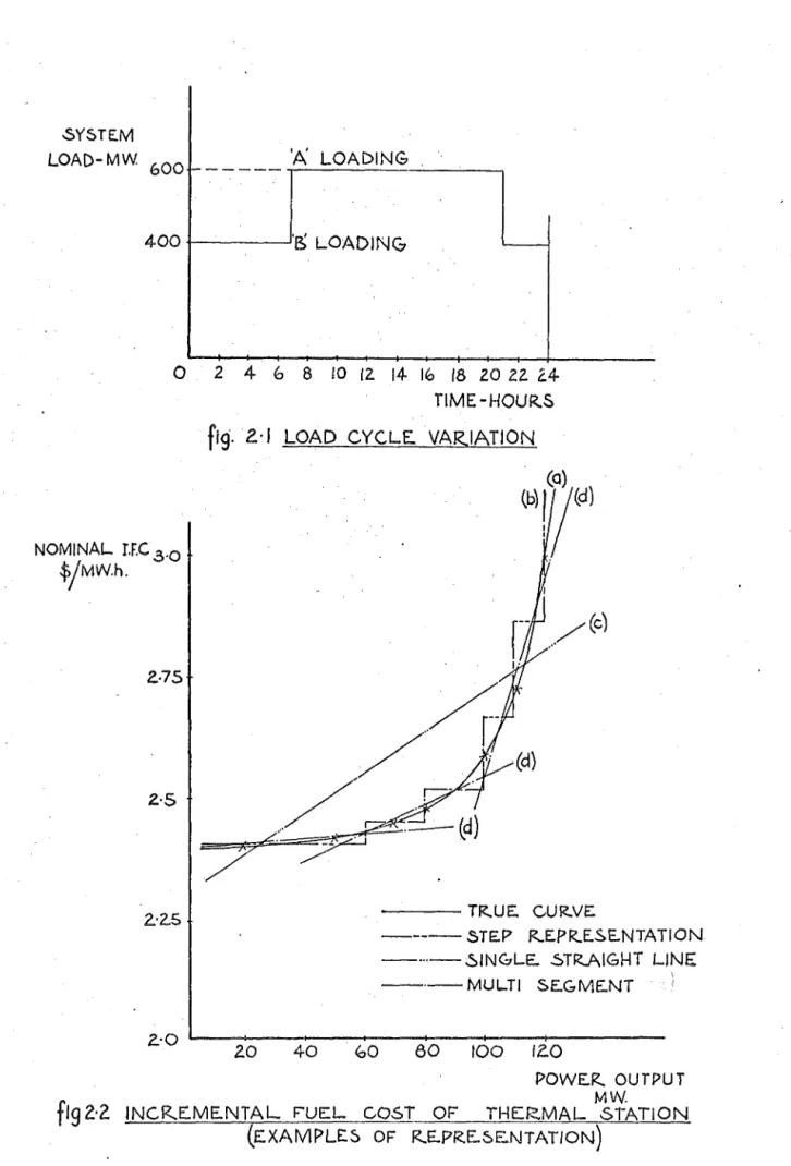
2,4 Load Demand Variation

The variation of the daily load cycle may be taken into account by subdividing the load cycle into a number of loading periods and calculating a set of B coefficients corresponding to each of these loading periods (figure 2,1). Each set of coefficients can then embody not only the load distribution, but also the typical system configuration

5

during that period. Kirchmayer and Stagg show that

although small variations occur between the B coefficients for the various loading periods because of changes in the loading period and generation parameters, an average value of these coefficients may also be applied over the whole daily load cycle without significant change to the optimum schedule,

2.5 Derivation of Incremental Plant Cost 2,5,1 Thermal Plant:

Incremental fuel rate =

in the limit =

6 ~input)

Li output) d

t

input) doutput)

The incremental fuel cost is then equal to the incremental fuel rate x fuel cost.

I.F,C, ($/fYlWh) = Fuel Cost ($/BTU x 106)

x I.F.R. (BTU x 106/fYlWh)

The representation of the incremental fuel cost for calculation purposes can be done in several ways of which the most usual

are:-(i) Step representation

(ii) Single straight-line approximation

(iii) fYlultisegment approximation as an extension of (ii) See figure 2,2 (example, fYlarsden Power Station).

The step representation is rarely used for thermal plant because of the steadily increasing characteristic of the incremental fuel cost. The straight-line approxima-tion is favoured, if a close approximaapproxima-tion can be obtained, as it simplifies calculation. As increasing accuracy is required, "higher order" representation is necessary leading to multisegment approximations3 to avoid significant loss in operating economy, but more sophisticated computing techniques are then required.

The straight-line equation for the incremental fuel cost is simply stated

-dF

n

dP

n

F

SY5TEM

LOAD-MW.

600 ,__ _____ 'A LOADING

400

+----__,·5

LOADlNG

-0

NOMINAL r.F.C .3·0

!f>/MW.'n.

?_.75

Z·S

2:2.5

2 4 6 8 10 12. 14- 16 18 2.0 2.2. ~4

TIME-HOUR.S

fig.

2.· I LOAD CYCLE. VARIATION

. (a)

(b)

!

/(di

... /(c)

- - - TR.UE'. CUR.VE.

- - - - S T E P R..EPR.E.SE.NTATION - · .. -SINGLE. 5TR.AIGHT LINE

~-·-MULTI SE.GME.NT . !

Z.:O .___ _ _ _ _ _

-..---+--~---t---2.0 40 ~o

eo

100 1z.o

POWER. OUTPUT

f

lg2·2 lNCR.E'..ME.NTAL F"UEL COST OF THERMAL srATION MW

where p ₌ ·generation of thermal plant n n

F = slope of incremental fuel cost curve nn

f ₌ intercept (constant term) of I.F.C. curve n

For multisegment representation this is extended·-dFn

F p f _Lo ·~ p _{~ L1}

dP

_n = nn₁ n + _n1 n

dF _{. n}

F p + f _Lk-1 ~ p

"

Lk

dPn = nnk n nk n

where L

0 , L1. o • • Lk are generation limits defining the range of each segment.

k = number of segments1

, .

From the station input/output curve, the station heat rate curve can be obtained as the derivative of the input/output curve, From these curves the incremental fuel rate curve is derived.

See figures 2.3, 2.4 and 2.5. 2,5,2 Hydro-electric Plant:

Tho incremental plant cost of a hydro plant is usually considered as the incremental water rate x the water cost,

I.P.C. ($/MWh) =water cost ($/106 cu.ft) x I.W.R.

(cusses/MW) x constant (sec/hr x 10-6)

dWn dP .

n

HEAT INPUT

S>TU/Hr

HEAT-IZATE.

BTU/MWh

INCR.EMENTAL xl08

14

12.

10

8

6

4

2. ...

0 2.0 40 60 80 100 12.0

POWER. OUTPUT - MW

f19.

2.·.3 INPUT/ OUTPUT CUR.VE.

>( 10

lo·O

~

14·0

13·0

12:0

11·0

10·0

9·0

zo

40 60 80 iOO 12.0

fiq.

2.·4

HE.AT RATE

POWE.R. OUTPUT-MW CUR.VE.

FUE.L fl .... ,A.. TE. .>: !

I

BT.UjMWh 11'0

10·0

9·0

8·0

'---t---...----20 40 60 80 100 120

POWER.. OUTPUT-MW.

In a manner similar to that ihown for thermal plant, the incremental water rate can be represented by

-(l')

St _{ep approx1ma ion} . t' g

(ii) Single or

multisegm~nt

straight-line approximations10 and the appropriate form of the hydro co-ordination equation obtained (figure 2.6).

The basic hydraulic characteristics inherent in hydro plant (head, tailwater losses, etc,) alter considerably the shape of th~ basic curve compared with the equivalent thermal p;ant.

If the incremental plant costs are considered rigorously, then in calculating the cost component the incremental cost of labpur and maintenance should also be included, However, as these costs are often difficult to extract as a function of output, they are normally neglected, or a small arbitrary amount included in the constant term. 2,6 Complete Solution of the Co-ordination Eguations

To obtain the economic schedule for a given time period, the co-ordination equations must be solved for each interval within that specified time period, thus in a 24 hourly

schedule, they are solved 24 times,

In addition to the constraints already discussed (load demand and water allocation) the individual station generation

The ref ore

P.

~

1

p . ~

-1

P.

P.

1 1

P.

P.

J J

<

i

₌

1 _{• ·, • • • • •ex}

~ j

₌

0( ₊

1 ' t t e I I~

where P.

1 = thermal generation of plant i

P.

J = hydro generation of plant j

and

P:-,

~' and P., P. are the maximum and minimum limits

1 J -2:. _.]_

respectively of P. and P. (figure 2o7),

1 J .

To enable the solution of the equations rearrange them,

P.

_l

=

p . c: J

From equation (7a) and (Ba)

ex:

f.

1

1.

o -

J..

- 2 (

2!

m=1 m i

w.

1.o -

Dj

t

-

2

Oj

8. lm

F ..

11

T

(

_2:

~

+

n=C(+1 n

w ..

-L1 ₊

1'

2

2

8 .. 11

<$..

Psm)

8. _{PHn +}

_2:

8.

Jn _m=1 Jm

8 ..

JJ

for thermal and hydro g~neration respectively. The equations can now be solved iteratively for P. and P .•

l J

The almost universal method of solving these equations is that of Gauss Seidel iterative method, with ~·held

J

( 1 0)

( 11 )

CIJSE.C5

/MW

116

114

112.

11,0

108

106

104

102.

20 40 60 80 100 12.0 !40 160 180

zoo

2.2.0

POWER. OUTPUT MW

f19.

2.·6 INCR.EME.NTAL WATER. R.ATE.

(AVIE.MORE P.S.) .

2.·JO CON~TANT 'Q''~

Z:OO

1·90

l·BO

1·70

H:iO

I ·55 '--li--+--+---t--1--+--+--+-l---lf--+-+---l--+--+--1--4~

ZO 406080100 I 40 ISO 2.2.0 2.hO .300

OUTPUT P4 MW

EFFE.CT OF GENE.R,ATION LIMITS

Therefore discussion has been restricted to the use of the Gauss Seidel method.)

In calculating the station generation, the generation limits must be satisfied. If no restriction is placed on the generation obtained from the solution of the equations, then the equations may yield negative generation, or

generation outside the specified generation limits. To satisfy these limits, when such generation values occur,

~hey are replaced by the appropriate limit value, and the equation for that particular station removed from the set of equations.

Further iterations in

i\

can then proceed in order to satisfy the load demand constraint.

2.6.1 Calculation of]\:

There is a unique value of

A

which satisfies the 'load demand. In solving the equations this value of

A

is

determined iteratively starting from an estimated value with its corresponding system load, and iterating with new values of

A

until the demand is satisfied. Several methods have been used to search for the correct

A

value.

(i) Dandeno10 used a step by step

A

increment procedure until successive values of

A

p~oduced deviations from the constraint of opposite sign, calculated the midpoint deviation and applied a second order Lagrangian

(ii)

correct, he applied an increasing order of polynomial until the correct

A

was located. To ensure

computa-tional stability, good starting values of

A

were required. 3 11

Kirchmayer ' suggested a linear interpolation having selected two values of

A

and calculated the deviation

-= +

where superscript i

₌

i-1

₌

i-2

₌

and _PR

₌

PR d

=

iteration iteration preceding received

p i-1 R being just

p i-2

R

started completed iteration

power ( :2P _n

-

_PL) power demand required

(Scheduling on total generat~on can be done equafly well (substitute PT for PR) and has the advantage that the system transmission losses do not require calculation during the

A

iteration.) This linear interpolation is used extensively to calculate the new

A

in a number of references and is used in this report.

( 1 2)

2.7 Calculation of Base Case Schedule

The above procedures are repeated for each time

interval and the schedule obtained for the estimated values

of ~'s. This first schedul~ if the water constraints

have not been sa ti sf ie d, be comes the base case s che du le

2.7.1 Correction of i~ to meet Water Constraints:

Theo's are the multipliers which are assigned values and determine the amount of water used. If the water constraints are not satisfied at the given plants, then the .~s are modified ·based on the deviation or residual amount of water (i.e., the difference between the water used and the water allocated). The calculation required to provide the modified values of the~~ takes much longer than that for the value of

A

as each time the

os

are

changed a complete trial generation schedule must be calculated, An additional complication stems from the fact that the water used at each plant is a function of all ~~ and therefore a linear interpolation of ~ can not be applied.

The usu al approach in cal cu 1 at ing the o's to meet 'the

1 0

water constraints is that described in detail by Dandeno , which considers the change in water used at each plant for a change in

o

at each constrainted plant.

A set of linear simultaneous equations are set up, the number of the equations equalling the number of plant for which there is a specified water allocation. The coefficients of these equations fo~m a Jacobian (or func-tional determinant) and the equations solved for values of

J'?S

(the correction for o) to reduce the deviation to zero. The linear equations are derived from the Taylor

f(x + dx)

₌

f(x) +

Jx

f'(x) +

!~~

f"(x) + •••••• The Jacobian assumes all stations are independent (the self or diagonal terms) for a change in ~ and then corrects for the effects of the existing dependence (the mutual or off-diagonal terms) in assuming =

f(x + dx)

=

f(x) + /x f'(x) the first order Taylor expansion,

Repeated application of the procedure may be necessa~y

to satisfy the constraints as the coefficients are linear approximations to f'(x). The equations are non-linear in fact since

-(i) the water flow is a quadratic function of the generation

(ii) the generation limits for each time interval may limit the change of generation for a corresponding change in

o

resulting in errors in the coefficient calculated.

( iii) The water used at each p 1 ant is dependent on a 11

O'

's • As an example, for a system with two constrained hydro plants, the foilowing equation would apply

-t\Q 1 1

b.

't

2

AQ 1

2

where

-AQ1

=

(water used at Plant 1 ) (water used at Plant 1

~

(in Base Case (Case 0) ) (in Case 1

b ~1

=

( ~for Plant 1 in Base ) (~for Plant 2 in

~

(Case ) (Case 1

AQ 1

₌

_{(water used at Plant 1}

~

(water used at Plant 2 )

1 _{(in Base Case (in Case}

2 )

R1

=

·(water used at Plant 1 ) (water allocated for )

(in Base Case ) (Plant 1 )

AQ2

=

(water used at Plant 2 ) (water used at Plant 2 )

(in B.ase Case ) (in Case 1 )

~02 ( l) for Plant 2 in Base \ _{· (~for Plant} ') . _{in l}

=

₎

<-)

(Case (Case 2

AQ 1

₌

_{~water used at Plant 2}

~

.

~water used at Plant 2

~

2 _{in Base Case}

in Case 2

R2

=

(water used at Plant 2 ) ~water allocated for

.(in Base Case ) Plant 2

ahd BASE CASE

₌

first schedule with estimated

os

CASE 1 schedule obtained for ~/

perturbation

=

61

CASE 2

₌

schedule obtained for

_~2

perturbation

and hence the new values of

₀

may be calculated

-0

1

ne~

=

O

1 old +

J~1

~2

=

new

~

2

old

+

!~2

solution of the linear sim~ltaneous equatioris, With the new

~ values a new schedule is calculated and the water used tested for convergence on the allocated .w~ter constraints, If these constraints are not satisfied this trial schedule becomes the

~ew Base Case and the procedure is repeated (flow diagram, figure 2,8),

The Jacobian coefficients AQ/~~ which are derived from the assumed linear relationship become less accurate the

turther the initial estimates of ~ are from the desired value, because of the effect of the generation limits, To overcome this problem, the ~ estimates should ideally be close

estimates initially but with a number of K's required an intelligent guess becomes mote difficult, hence several techniques have been developed to prevent breakdown of the· procedure if the

~s

are not accurately estimated1 D, 12

These techniques will be described in Section 3, 2,8 Summary

An outline of the method of equal incremental costs for the economic generation scheduling in an integrated system · has been presented showing

-(a) the basis of the method and ·its validity for economic scheduling,

(b) its shortcomings, and,

POWE.R LOOP

LAMBDA LOOP

TIME:. LOOP

GAMMA LOOP

INPUT DATA

PLANT

INCREMENTAL

t..055E.S

PROCE:.E..P TO

NE..XT PLANT

ADJUST J\

PROC.E.E.D TO

NE.XT HOUR..

ADJUST ~S

PLANT

INCRE.MENTAL

COSTS

PLANT

G!::.NERATION

PRINT GE.NE.RATION

SCHE:.DULE.

SECTION 3

DIGITAL comPUTER PROGRAm LANZOP

3.1 Introduction

To implement economic load allocation for the New Zealand Power System, in the preparation of this report, a digital computer program (LANZOP) has been developed using the method of co-ordination equations discussed in

~ection 2 on a model of the South Island System. The program has been written in FORTRAN IV for use on the I.B.m. 360/- series computers,

The aim in the designing of the program and its operation has been to provide a tool for the use of the System Control Operator. The output from the program

should satisfy his requirements for information in quantity and quality for effective use, This information required for input should be restricted to essential data, such as the daily load curve, water constraints, and water values which cannot be derived otherwise, As discussed in Section 2, good starting values of water cost (~) and incremental .cost of received power (A) may reduce the computing time,

generation limits, plant characteristicswhich generally have unchanging values are set up with the standard values, but with provision for modification as required. These features have effectively reduced the input quantity and relieved the operator of much detail. Part of the reason for this minimisation of data being done was the likelihood of the program being operated from a remote console, which being a relatively slow speed device is not suitable for extensive data transfer.

3.2 The System Model

The South Island System has been modelled by a six busbar system representing a simplified version of the major transmission lines and their interconnections, with four generation busbars (figure 3.1).

The bus bars are referred to as follows:-. Busbar

No. Name Major Components Function

1 Waitaki Benmore, Aviemore, Waitaki Generation,

(Basin) Load

2 Highbank/ Highbank and Coleridge Generation Coleridge

3 Cobb Cobb Generation,

Load

4 Roxburgh Roxburgh Generation,

Load

5 Livingstone Livingstone Switching

6. _{Islington Islington Load}

J: WAITAKI

3: COBB

D.C.LOAD

4: R.OXBUR.<;H

AC.LOAD AC.LOAD

AC.LOAD

A.C. LOAD

,5: LIVINGSTONE 6: ISLING TON

to some extent for lines which are not directly modelled by the system.

The model was chosen to facilitate the development of the computer program for scheduling and to give reasonably accurate results which could be compared with actual

schedules obtained from the system. The major simplification was the combining of the Waitaki Basin generation sources

into one plant on the Waitaki River. This simplification is valid as the stations are close together electrically and the generation scheduled for each hour would normally be the total output required from the Basin, as the distribu-tion of generadistribu-tion between the individual stadistribu-tions is

optimized on a different basis13' 14 as the stations are considered operationally as a su~system,

3,3 Transmission Losses

It has been shown that the inclusion of transmission losses results in improved ec?nomy. The loss formula method using B coefficients has been used in this program to calculate the incremental and full transmission losses, A computer program LFBCDP15 (developed previously using Kirchmayer's method3)

p~ovided

the B coefficients required for use in the pr6gram LANZOP, The coefficients describe the model of the system as outlined in 3.2 above, For typical results refer to Appendix B.

3,4 Implementation of the Co-ordination Equations

This section will follow closely the sequence of Section

3.4.1 The Organization of Program LANZOP:

The co-ordination equations consist of a set of four equations corresponding to the four generation busbars in the system model, hence the. four busbar program,

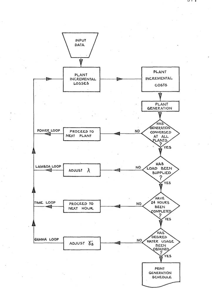
The flow diagram, figure 2.8, indicates the basic

sequence of the generation scheduling programo The program has been org~nised as a single phase program and during

execution, the entire program remains in core storage,

~squiring approximately 25K bytes of storage of which 3K bytes are needed for data storage. The output information is displayed on a lineprinter while all input is entered from the cardreader, The output data has been kept to a minimum and besides the hourly generation schedule, consists of a check listing only-of the load curve, water constraints and water values, and any diagnostic messages for the

operator. The program listing and symbol list is contained· in Appendix A,

The components of the program

are:-(i) Subprogram BLOCK DATA - this subprogram initializes all the parameters named, with the values defined, setting up the so-called standard values (or options). These values are changed as required by card input, The number of time intervals A (= 24), the plant

ch~racteristics WP, WC are typical examples of the parameters initialized with standard values,

(iii) Subroutine CENALL - the subroutine which calculates the generation schedule.

(iv) Subroutine PAREQ - the subroutine which solves the linear simultaneous eq~ations for /~ and hence the new values of

o.

(v) Subroutine MINV - the subroutine which inverts the Jacobian matrix as required by PAREQ (Standard I.B.M. Scientific Subroutine)o

In addition to these essential program blocks,

subroutines have been written which will graph the generation schedule and the individual station schedules on the line-printer for convenience (subroutines PLOTC and GRAPH), but as they are very time consuming due to the relatively slow speed of the lineprinter, they are normally omitted and therefore no further reference will be made to them. 3.4.2 Data Input

-The minimum data required for successful execution of the program

is:-(i) Daily load curve

I , , \

\l.l.J Estimated '1.-:::ll11oc

V U.J..ULI '-'

(iii) Specified water constraints {water allocation) In addition, (iv), any nonstandard values for initialized parameters, and good starting values of

A

may be necessary or desirable.

constraints for feasibility, based· on the specified generation limits, and if necessary are reset to the appropriate limit.

3,5 Calculation of the Generation Schedule

The f lo~ diagram for the calculation is shown in figure 3.2.

3.5.1 Calculation of Plant Generation:

Tha co-ordination equation for each plant is solved by the Gauss Seidel iterative method16 in the form

-w

pn

=

1.0 - 'o'n

A

w

_nn

T

n

2 ~

m=1

m n

+ 28 nn

B p

mn n

where P

=

generation for hydro plant n

n

since direct solution is not possible. Computational experience has shown that the inclusion of the incremental transmission losses and hence the B _nn term in the scheduling equation, results in a computationally more stable system, and the equations always converged, Comparative schedules were made neglecting the losses and considerable difficulties arose in attempting to converge on the specified water usage, and in several cases convergence was not achieved.

TIME. LOOP

GAUSS ..

SET HOUR. •

E.~TIMATE'.. A F~OM

INl>UT OATA OR.

PREVIOUS RESULTS

CALCULATE. PLANT GS:NE.RATION

(Pn)

SE.IDEJ...

ITE.RATIVE. LOOP

A

ITE.R.ATIVE.

LOOP

NO

sn:p CHANGE IN

s

A

F'OR. NEW

A

INC.RE.ME.NT .HOUR.. &Y I

YE.5

NO

f19 .

.3·2. GE.NE.~TION Sc.,HE.DULE.. FLOW DIAGR.AM.

LINEAR INTE.l<:,POL.ATION

FOR NE.W A

E.XIT

SUBROUTINE. GE.NALL

&.___¢, i\

ITERATIVE. LOOP~,

t t . t' . 'f' tl 17 compu a ion ime s1gn1 ican y of P are modified thus

-n

The succ~ssive values

p i-1

n

=

p i-2. +

n (

i-1

p . _P i-2 ). _{x acceleration factor}

n n

where i-1

=

iteration ju~t completed, etc,

Typical valu~s of acceleration factor are Oo3-0,6.

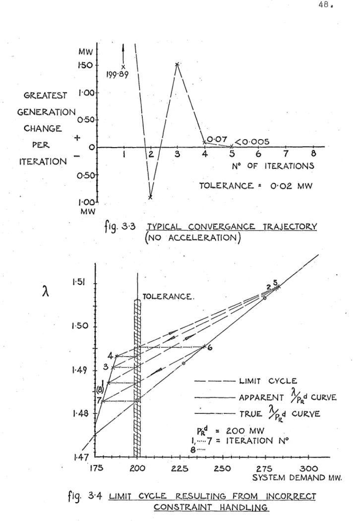
For this application, extensive testing of the Gauss Seidel iteration was carried out with varying acce1.eration factors, tbs result of which showed that in this system, the use of an acceleration factor increased the number of iterations required for convergence, by causing oscillation of the convergence trajectory.

Typically

-the number of iterations required without acceleration

=

5 the number of iterations required with acceleration

₌

10

(Acceleration factor

=

0,35)

where e

=

tolerance

=

0,005%

See figure 3. 3.

To initialize the Gauss Seidel solution, the initial values of p have been set to p •

n n In practice, these limits

were often exceeded during the first few iterations. If the limiting values were substituted immediately and the number of equations reduced then a solution in which the

true valua of ·p was just inside the limit was often excluded.

n

coincide with the value required for convergence. To overcome this serious problem, the limit substitution was made, but the equation left in solution for the first and second iterations,

An earlier method of handling the generation constraints in the Gauss Seidel iteration, by substituting any limit

values only after the first iteration had been completed, proved most unsatisfactory. Th~ apparent solution induced oscillation in later iterative loops and convergence on the System load demand became unattainable since an iterative "limit cycle" resulted. See figure 3.4. This condition was accentuated by the.use of a linear interpolation formula for

fi.,

(Reference Section 3.5.2 .• )

3,5,2 Calculation of..i\:

Convergence having been achieved for the solution of the generation values P , the total generation, the

trans-. n

mission losses, and hence the received power PR were calculated for the current value of

.A,

i.e.,

=

At this point, the solution is tested for the satisfying of

d

the System load demand PR , i.eo,

Is

₌

where e

=

p d

R + e ?

tolerance specified

If this is not satisfied then iteration of

A

proceeds (with the consequent recalculation of the generations) until

.

MW J·SO

GR.E.ATE&T 1·00 GENE.RATION

0'50

CHANGE.

+

0·5

f·OO.

MW

1·51

1·50

1·49

1·48

/

/

1 \

199·89 \

\

\

2.

\ I

y

N° OF' ITE.R..ATIONS

TOLER.ANCE. = 0·02. MW

fig.

3·:3 TYPICAL CONVER.GANCE. TR.AJE:C..TOR.Y

(No

AC.CE.LE.R.ATION)

/

/

1·4 7

L...-t--+-+--t-~+-+-1-4-+---l-+--+-+-+-+-t-~-+--+--+---i--' 175

zoo

_{Z..2..5 250 Z.75 300}

SY5TE.M DEMAND MW.

From the results of a large number of schedules it was shown that an estimated

A

value close to the true

value of

A

which satisfied the demand, significantly reduced the convergence time. Consequently in the selection of ~~

for the perturbation schedules (i.e~, the schedules calculated in deriving ~Q/~~) and the new base case schedule, the

results of previous iterations and the change in o(s) have been used to make closer estimates of ~ for the trial schedules. To date, the effectiveness of the estimating technique is somewhat limited·if the values of~ are

significantly different from the average values used, as the numerical constants used in the estimation have been derived from analysis of previous experimental results and are not dynamically updated.·

To aid convergence, a set of

A

values are calculated to act as reference points. These reference points are the calculated

A

values at which the plant generation limits are imposed and are defined by

-"A n

=

Y x (W x P

on nn n

1-2

·2::

B P

rnn m

+

w )

n

for example, refer figure 3.5.

From this definition a set of guide points is found. for P

= P

and P

=

P respectively

n n n n

3·2.S

. I\

3·00

2:75

l·SO

2.·Z.S .

Ji.

~EVER.SAL- EFFE.C T OF

NEGATIVE. INC~E.ME.N TAL

LOSSES

Pl

PZ. P3

P4

1'

SYSTEM

i\

= minimum value of

A

for minimum generation P at plant n . ...!J.

and then obtain

A

and ~ being the maximum ~n and minimum An respectively to define the expected range of

A.

Procedure for Crinvergence on Demand -(i) Estimated value of

.A

input as data.

The plant generation outputs for this value of

_A

are calculated and from the deviation (PR

-

pRd) a step change· of )... is made in the correct direction.

X

=

A

est +

AA

where

_t::.A.

_{= Const x Asst x SGN (PR d}

-

_PR) and SGN (PR d PR) = +1 _PR d

_>

_PR

= 0 _PR d _=PR

-1 d

= PR (. PR

and a new trial schedule obtained. If the power

received (PR) has changed then the linear interpolation formula (equation 12, Section 2) is applied.

interpolation is repeated until

I

pRd - PRI

~

e where e = specified tolerance.

(ii) Estimated value of

A

not input as data.

The trial schedule for

A

is calculated and then iteration proceeds as in (i) above.

A

number of factors may make this procedure

unsatisfactory:-(a) Demand outside range of generation

-i. 8 . '

2:

p

_n

<

p _R d or

2:

p _n

>

p _R d Thi~ prevents convergence. This condition is

This

iterations and has a value

A

=

6

or

A=

~ for both iterations, and the program terminates on this occurrence. Since this is an unlikely condition it is not tested for directly during the data check, (b) Slow Convergence

-This can occur if there is a large disparity between

~reference points wjth no change in generation (see figure 3,6) and the deviation is small (just greater than e) with a consequently small

6A•

In this event, the program searches for the next significant

A

reference point and proceeds. Convergence is then normally achieved within several further iterations. (c) Solution of the Simultaneous ~quations resulting in

negative

os

-The

A

reference points for some plant become inverted and the

A

iteration breaks down, In this event, the

~'s are tested and reset to the equivalent of 5% change and the plant output schedule (trial schedule)

recalculated,

3.5.3 Calculation and Adjustment of ~ {Camma2:

As outlined in Section 2, the

₀

values (water values) ·determine the water used at each hydro plant. If after

the first schedule has been calculated the correct amount of water has not been used, then the

os

at the plants constrained must be modified, The method used in this

10

3·00

i\

2:50

2.·00

l - 6 N° OF ITERATIONS

1·50

Pa

A

SYSTE.M

A

RANGE:.

flq. 3·6 USE OF

A

R.EFE.TZE.NGE. POINT6