Munich Personal RePEc Archive
Estimation of Technical and Allocative
Inefficiencies in a Cost System: An Exact
Maximum Likelihood Approach
Tsionas, Efthymios and Kumbhakar, Subal
November 2006
Estimation of Technical and Allocative Inefficiencies in a Cost System:
An Exact Maximum Likelihood Approach
Efthymios G. Tsionas Department of Economics
Athens University of Economics and Business 76 Patission Street, 104 34 Athens, Greece Phone: (301) 0820 3388, Fax: (301) 0820 3310
E-mail: [email protected]
and
Subal C. Kumbhakar Department of Economics State University of New York Binghamton, NY 13902, USA Phone: (607) 777 4762, Fax: (607) 777 2681
E-mail: [email protected]
This Version: April 2006
Abstract
Estimation and decomposition of overall (economic) efficiency into technical and allocative components goes back to Farrell (1957). However, in a cross-sectional framework joint econometric estimation of efficiency components has been mostly confined to restrictive production function models (such as the Cobb-Douglas). In this paper we implement a maximum likelihood (ML) procedure to estimate technical and allocative inefficiency using the dual cost system (cost function and the derivative conditions) in the presence of cross-sectional data. Specifically, the ML procedure is used to estimate simultaneously the translog cost system and cost increase due to both technical and allocative inefficiency. This solves the so-called ‘Greene problem’ in the efficiency literature. The proposed technique is applied to the Christensen and Greene (1976) data on U.S. electric utilities, and a cross-section of the Brynjolfsson and Hitt (2003) data on large U.S. firms.
JEL classification: C 31
1. Introduction
The standard neoclassical production theory assumes that producers are always efficient. This assumption,
however, is not consistent with reality. Consequently, the idea of measuring efficiency of firms is becoming popular
both in the government and private sectors. In measuring efficiency of producers, the focus is mostly on technical
efficiency, which is often associated with managerial efficiency and estimated form the production/distance functions
or the dual cost, revenue and profit functions. Although achieving technical efficiency is perhaps the utmost concern,
producers can be inefficient in using their input mixes as well. This is labeled as allocative inefficiency, which
increases cost. Thus a producer is economically efficient when it is both technically and allocatively efficient.
Estimation of both technical and allocative efficiency requires the use of a system approach. However, the system to
be used depends on type of data available and the behavioral assumption on the part of the producers. For example,
the cost system is appropriate if the assumption of cost minimization holds (as is the case with regulated utilities).
In the stochastic frontier literature there are two approaches to estimate a system and obtain measures of
increased cost due to technical and allocative efficiencies under the behavioral assumption of cost minimization.
First, the primal system approach was originally proposed by Schmidt and Lovell (1979). Their system, constructed
from a Cobb-Douglas (CD) production function and the first-order conditions of cost minimization, is used to
estimate the parameters of the model as well as technical and allocative inefficiencies. Since inefficiency increases
cost, measurement of increased cost due to each type of inefficiency is needed. This requires knowledge of the cost
function, which for a CD production function can be easily derived analytically. Once the cost function is derived,
computation of increased cost associated with technical and allocative inefficiencies (using the estimated parameters
and estimates of technical and allocative inefficiencies from the primal system) is trivial.1 The second approach is to
estimate the dual cost system and was first suggested by Greene (1980). There are two problems in this approach,
especially when a flexible functional form is used. The first problem is related to specification of the cost function
that accommodates both technical and allocative inefficiency and the second problem is related to joint estimation of
the cost system and computation of cost increase due to each inefficiency component. Note that these problems are
not trivial even for production functions for which the cost function can be derived analytically2, unless one uses the
1 Although the Schmidt-Lovell procedure can be extended to accommodate flexible functional form such as the translog (Kumbhakar and Wang (2006)), it is not possible to derive the cost function analytically. That is, for flexible production functions computation of cost associated with technical and allocative inefficiency is not trivial.
Schmidt-Lovell (1979) primal system to estimate the model and then uses the analytical cost function to compute cost
of each inefficiency components. In other words, although the dual cost system helps one to specify the technology
and identify costs of each inefficiency component, estimation of such a system using cross-sectional data is yet to be
done.3
Kumbhakar (1997) solved the specification problem in a dual cost function framework that incorporates
both technical and allocative inefficiency in any cost system. This formulation uses an input-oriented technical
inefficiency specification and introduces allocative inefficiency following Schmidt and Lovell (1979). It solves the
specification problem theoretically; however, no estimation technique is offered. The difficulty is that the cost
function and the deviations of optimal shares from their observed counterparts are complicated functions of allocative
inefficiency. Although the link between allocative inefficiency and increase in cost therefrom is well established for
any cost function in Kumbhakar (1997), the stochastic structure for the cost system consisting of the cost function
and the cost shares is, unfortunately, very complicated for the standard ML method. This estimation problem has
been a major stumbling block for more than two decades and is labeled as the Greene problem by Bauer (1990).
It is often argued that the Greene problem can be circumvented if decomposition of cost efficiency into
technical and allocative components is not desired. The logic behind this argument is that since both inefficiencies
increase cost inclusion of a one-sided error term in the cost function will capture the cost of overall (technical plus
allocative) inefficiency, which can easily be estimated by the standard ML method using a single equation approach.
However, it is shown by Kumbhakar and Wang (2005), in terms of a detailed Monte Carlo simulation, that failure to
include allocative inefficiency explicitly in the cost function biases estimates of (i) the cost function parameters, (ii)
returns to scale (RTS), (iii) input price elasticities, and (iv) cost-inefficiency. They also found that the true and
estimated distributions of RTS, elasticities, and cost-inefficiency are quite different. Based on these results they
concluded that the widely held view that ignoring costs due to allocative inefficiency (or aggregating it with the cost
of technical inefficiency) is not likely to affect the technological parameters and measures of RTS, elasticities, etc., is
not correct. These findings send a strong message indicating the importance of solving the Greene problem, i.e.,
estimating costs of technical and allocative inefficiency jointly from a system.
We are not aware of any application where the Greene problem is solved using a flexible cost function and
cross-sectional data with the exception of the Bayesian approach in Kumbhakar and Tsionas (2005). Empirical
application of the Kumbhakar (1997) model in a sampling theory framework is difficult because of the complex error
structure of the model, especially when allocative inefficiency is represented by random variables a la Schmidt and
Lovell (1979).4 Because of this difficulty no one has applied the method proposed in Kumbhakar. In this paper we
propose a classical solution and use an exact ML approach to estimate the translog cost system in a cross-sectional
setup where both technical and allocative inefficiency are random variables. The proposed method solves the long
lasting Greene problem.
The rest of the paper is organized as follows. The cost system of Kumbhakar (1997) is briefly presented in
Section 2. The ML estimation procedure is discussed in Section 3, first with only allocative inefficient and then both
technical and allocative inefficiencies. Data and results are discussed in Section 4, followed by some concluding
remarks in Section 5.
2. The model
Since our focus is to estimate the cost system, in this section we lay out the model proposed in Kumbhakar
(1997). Let the production technology be specified as where qi is output and xi is a vector of J inputs
for firm i (i = 1, …, n), f (.) is the production function, and measures input-oriented (IO) technical inefficiency
(Farrell (1957)). This specification implies that a technically inefficient producer over-uses all the inputs by u ( ui
i i
q = f x e− )
0 i u ≥
⋅100
percent compared to an efficient producer producing the same output. Consequently, the IO measure of technical
inefficiency is useful when the objective of the producers is to allocate inputs in such a way that cost is minimized for
an exogenously given level of output. In allocating inputs producers may make mistakes. These mistakes are labeled
as allocative inefficiency. Here we follow Schmidt and Lovell (1979) and Kumbhakar (1997) in modeling allocative
inefficiency, viz., , Here a non-zero value of
1 , 1,
( ui) / ( ui) j i/ , 2,..., .
j i i j i i
f x e− f x e− =w eξ w j= J ξj i, indicates the presence
of allocative inefficiency for the input pair (j,1) for firm i. Note that unless the production function is homogeneous
the IO technical inefficiency term (u) will not drop out from the first-order conditions.
4 With panel data these problems can be avoided by modeling allocative inefficiency parametrically. This involves the assumption
Schmidt and Lovell (1979) used the above framework to estimate a Cobb-Douglas production function for
which the cost function can be derived analytically. Since there are not many production functions for which the cost
function can be derived analytically and the interest is mostly on costs of inefficiency, the natural alternative is to
consider a dual cost function, which is widely used in empirical studies. The cost function specification with
input-oriented technical inefficiency is strongly separable in costs of technical and allocative inefficiency. The
complicating factor is that the cost share equations are affected by the presence of allocative inefficiency. Thus, the
model has to take into account the link between allocative inefficiency appearing in the cost share equations and
increase in cost therefrom that appears in the cost function. The modeling approach proposed by Greene (1980) did
not make use of this link in a theoretically consistent manner. Kumbhakar (1997) derived the exact relationship
between allocative inefficiency and cost therefrom using a translog cost function, thereby solving the Greene problem
theoretically. This relationship is crucial from estimation point of view because it connects the error terms in the cost
share equations and the cost function.
Since ξj i, represents allocative inefficiency for the input pair (j, 1) the relevant input prices to the firm i (i =
1, …, n) are * ( , i
w ≡ w1,i w2,iexp(ξ2,i),…,wJ i, exp(ξJ i,))′ where ξ2,i,...,ξJ i, are random variables that capture
allocative inefficiency. Kumbhakar (1997) showed that actual cost could be expressed as
* *
ln a ln ( , ) ln ( , , )
i i i i i i
C = C w q + G w q ξ +ui
j
C = ∑ w x C w q*( *i, )i
-u
(1)
where and is the minimum cost function obtained from solving the following problem:
. The G(
, ,
a j
i j i i
*'
min subject to
u i
u
i i i i
x e
w x e q f(x e )
−
− = , ,
i i i
w q ξ ) function in (1) is defined as where
. Since (1) is strongly separable in , cost of technical inefficiency (percentage increase in
cost due to technical inefficiency) is represented by . The allocative inefficiency terms (
, *
,
(.) j i
j j i G = ∑ S e−ξ
* *
, ln (.) / ln
j i j i
S = ∂ C ∂ w*, ui
0 i
u ≥ ξj) appear both in the
and the G(.) functions. Thus, to separate the cost of allocative inefficiency, we need to define , the
cost frontier (also labeled as the neoclassical cost function). For this we rewrite the cost function in (1) as
where is the cost frontier (the neo-classical cost function),
which can be obtained from the cost function in (1) by imposing restrictions that firms are efficient both technically
and allocatively. That is,
*(.)
C C w q0( , )i i
0
ln a ln ( , ) ln AL( , , )
i i i i i i
C = C w q + C w q ξ +ui C w q0( , )i i
0
,
ln (.) ln a(. | 0 , 0)
j i i
ln AL( , , ) i i i
C w q ξ ln | 0 ln 0(.) ln *( *, ) ln ( , , )
i
a
u i i i qi i
C = C C w q G w ξ
= − = + −lnC0(.). The term can be interpreted
as the percentage increase in cost due to allocative inefficiency.
ln AL i C
To get a better understanding of the above decomposition we start with a parametric functional form
on . Once a functional form for is assumed, the G(.) and C0(.) functions can be easily derived. Using these
functions we can easily obtain . Since the cost function in (1) is naturally expressed in logarithms, it is
convenient to discuss both modeling and estimation issues in terms of the Cobb-Douglas and translog cost functions.
It is worth pointing out, however, that the methodology is equally applicable for any other flexible parametric form
for . For example, if we assume a parametric functional form (e.g., translog) for , i.e.,
*(.)
C C*(.)
lnCAL
*(.)
C C*(.)
(
)
2* * * 1 1 * * *
0 , 2 2 , , ,
ln ( i, )i jln j i qln i qq ln i jkln j iln k i jqln j iln i
j j k
C w q =α +∑α w +γ q + γ q + ∑ ∑β w w + γ w q j
∑
q
i
then . Imposing the linear homogeneity restrictions on , and noting that
by definition, we can rewrite (1) as
* *
, ln , ln
j i j jk k i jq i k
S =α +∑β w +γ C*(.)
* 1,i 1,
w =w ln( a/ 1,) ln *( *, ) J *, exp( , )
i i i i j i j i
j
C w = C w q + ∑S −ξ
) i
C w C w q C w q ξ u
, where
and . Now we write the cost function and the associated cost
share equations in terms of C0(.). These are
* * * *
1,
( i, )i ( i, ) /i i C w q =C w q w
2,
* * *
1, , 1,
( / ,..., /
i
i i J i
w = w w w w
0 1,
ln( a/ ) ln ( , ) ln AL( , , )
i i = i i i + i i i i + i, (2)
0
, ,( , ) ,( , , )
a
j i j i i i j i i i i
S =S w q +η w q ξ , i=1,...,n; j = 2, …, J (3)
where wi =(w2,i/w1,i,...,wJ i, /w1,i), , , , / is the actual (observed) cost share of input (
a a
j i j i j i i
S =w x C j j=2,...,J),
is the normalized (by ) cost frontier and ( ). For the above
translog cost function is
0( , )
i i i
C w q w1,i S0j i, = ∂lnCi0(.) / ln∂ wj i, j=2,...,J
0
lnC w qi( , )i i
(
)
20 1 1
0 , 2 2 , , ,
2 2 2
ln (.) ln ln ln ln ln ln ln
2
J J J J
i j j i q i qq i jk j i k i jq j i i
j j k j
C α α w γ q γ q β w w γ w q
= = = =
= + ∑ + + + ∑ ∑ + ∑
J
, (4)
, (5)
0
, ,
2
ln ln , 2,...,
J
j i j jk k i jq i k
S α β w γ q j
=
= +∑ + =
1
, , , 2 , , ,
2 2 2 2 2 2
ln AL ln J J J ln J J J ln ,
i i j j i jk j i k i jk j i k i jq j i i
j j k j k j
C G α ξ β ξ w β ξ ξ γ ξ
= = = = = =
{
}
0
, , ,
,
,
1 exp( )
exp( ) j i i j i j i j i
i j i
S G a
G
ξ η
ξ
− +
= , j=2,...,J (7)
where
0
, , ,
2
( ) exp(
J
i j i j i j
G S a ξj i)
=
= ∑ + − , (8)
and
, 2
J j i jk k i
k a β ξ ,
=
= ∑ . (9)
The cost system defined in (2) and (3) serves two purposes. First, technical and allocative inefficiencies are
modeled in a coherent manner. Second, the exact link between allocative inefficiency (ξj) and its cost is given in (6).
The cost function decomposes the overall increase in cost due to inefficiency into two components, viz., the
percentage increase in cost due to allocative inefficiency, , and the percentage increase in cost due to
technical inefficiency, ui. The decomposition formula also establishes an exact link between the error terms in the
cost share equations (which are functions of allocative inefficiency) and cost of allocative inefficiency, which is very
important from estimation point of view. In general, the link is provided by the relationship ln ln AL
i C
( , , ) AL
i i i C w q ξ =
* *
lnC w q( i, ) ln (i + G w qi, , )i ξi
0
lnC (.)
− . For the Cobb-Douglas case, this link is established in Schmidt and Lovell
(1979), viz., 1
2 2
ln ln j ln[ ]
J J
AL
1
J
j j j
j j
C e ξ j
j
α ξ
α
α
−α
= = ⎡ ⎤ = + ⎢ + ⎥− ⎣ ⎦
∑
∑
=∑
. Since Schmidt and Lovell used the systemconsisting of the production function and the first-order conditions of cost minimization, it was not necessary to use
the above link in estimation. It was, however, used to compute the cost of allocative inefficiency. Thus, Schmidt and
Lovell avoided the Greene problem by not estimating the cost system. Kumbhakar and Wang (2006) did the same
when they extended the CD model of Schmidt and Lovell to accommodate flexible production functions (such as the
translog). Although they avoided the Greene problem by following the Schmidt and Lovell procedure, they had to
solve a system of nonlinear equations to compute the costs of technical and allocative inefficiencies.
The Greene problem is associated with estimating a cost system in (2) and (3) using the link between cost of
allocative inefficiency and errors in the cost share equations (which are functions of allocative inefficiency), given in
equations (6), (8) and (9). Thus to address the Greene problem, we focus on estimating the cost system It can be seen
estimated using cross-sectional data.5 In the following section we discuss an estimation method, first with only
allocative inefficiency and then with both technical and allocative inefficiency.
3. Estimation
3.1. Only allocative inefficiency
For simplicity we consider first the case with only allocative inefficiency, and write the cost system in (2)
and (3) as
0
0
, , ,
ln ln ( ) ln ( , ) ,
( ) ( , ), 2,..., , 1,..., ,
a AL
i i i i i
a
j i j i j i i
C C C v
S S j J i
β β ξ
β η β ξ
= + +
= + = = n
(10)
where β is the parameter vector associated with the translog cost function, and v is the stochastic noise component
added to the cost function. To avoid singularity problem, one share equation is dropped and we normalize the
corresponding element of ξi to zero. We impose the standard distributional assumptions on the error components, vi
and ξi, in the above system.. More specifically, we assume
2
~ . . . (0, ) i
v i i d N σ and ξi ~ . . .i i d NJ−1( , )µ Ω , distributed
independently of . Here, the vi (J− ×1) 1 vector µ represents systematic allocative inefficiency, and the
matrix Ω is the covariance matrix of allocative inefficiency components. (J− ×1) (J−1)
We write the ith observation for the above system compactly as
ln ( , ) ( , )
AL
i
i i
i i i
i i i
C v
y X β ξ β Xβ ε
η η ξ β
⎡ + ⎤ ⎡ ⎤
= +⎢ ⎥≡ +⎢ ⎥ ⎣ ⎦
⎣ ⎦ , (11)
where ,
2, ,
[ln , ,..., ]
i J i
a a a
i i
y = C S S ′ Xi =[lnCi0( ),β S2,0i( ),...,β SJ i0,( )]β ′, η ξ βi( , )i =( (η ξ βi 2,i, ),..., ( , , )) 'η ξi J i β . Since the
error vector in (11) is ( , ) 'ε ηi i , for the ML method one has to derive the joint pdf of ( , ) 'ε ηi i starting from the
distributions on and vi ξi. The joint pdf of ( , ) 'ε ηi i is p( , )ε ηi i = pε η| ( | )ε ηi i pη( )ηi and
5 The system described in (2) and (3) is somewhat similar to the Kumbhakar and Tsionas (2005) model which assumed the
2
| ~ (ln AL( ( ), ), )
i i N C i i v
ε η ξ η β σ , where ( )ξ ηi i is the solution of ξi in terms of ηi fromη η ξ βi = i( , )i . Furthermore,
the pdf of pη( )ηi can be expressed as
( )i ( ( )). | deti i i( ) |
pη η = pξ ξ η Dξ ηi , (12)
where Dξ ηi( )i is the Jacobian matrix (derivatives of ξi with respect to ηi). Therefore, the joint pdf of the error
vector in (11) is
/ 2 2 1/ 2 1/ 2 | 2 1 1 2 2
( , ) ( | ) ( ) (2 ) ( ) det( )
[ (ln ( ( )]
exp ( , ) ( , ) | det ( ) |
2
J
i i i i i v
AL
i i i
i i i i i i
v
p p p
C
e e D
ε η η
ε η ε η η π σ
ξ ξ η η β η β ξ η
σ
− − −
−
= = Ω ×
⎧ − ⎫
⎪− − ′Ω ⎪
⎨ ⎬
⎪ ⎪
⎩ ⎭
(13)
where ( , )ei η βi =ξ η βi( , )i −µ.
In practice, to implement the likelihood function based on (13) we have to show that (i) ξ can be solved in terms of
η, and (ii) the Jacobian matrix can be derived analytically. We show these next.
For notational simplicity now we drop the observation index i. The first task is to solve for ξ in terms of
η. Note that
0
a j Sj Sj
η = −
0
1
[1 exp( )]
exp( ) J
j j jk
k
j
S G
G
k
ξ β ξ ξ =
− + ∑
=
0 0
1
( j j) exp( )j j J jk k k
S G S
η ξ β ξ
=
⇒ + = + ∑
0 0
1 2
exp( ) J J
a
j j j jk k j jk k
k k
S G ξ S β ξ S β ξ
= =
⇒ = +∑ = +∑ , j=1,...,J. (14)
For the last equality we used the normalizationξ1 =0. The equations in (14) can be expressed in ratio form to
generate the following system of nonlinear equations,
0 2 0 2 exp( ) J j jk k
k
j j J
J Jk k k S S β ξ λ ξ β ξ = = + ∑ =
where a/ 1a. In the Appendix we use fixed point arguments to show that a solution of j Sj S
λ = ξj exists and is unique.
Once the ξjs are obtained, the value of G can be obtained as
0 * 1 1 2 1 1 1 J k k k a S S G S S β ξ = + ∑
= = a . Note that we need to
compute
G
ln AL( , ) i C ξ β .
The second task is to derive the Jacobian of the transformation from ξ to η. To compute it we start again
from the definition of ηj, i.e.,
0
2
(1 ) J
j j ik k
k j j S h h β ξ
η = − + ∑= j=2,...,J
j
, , where hj =Gexp( )ξ . Differentiating it with respect to ηl gives
j
a k
j jl j jk
k k
k l h
h S k
l
ξ ξ
δ β
ξ η η
∂ ∂ ∂
+ ∑ =∑
∂ ∂ ∂ , (16)
where δjl is the Kronecker delta. The system in (16) can be written as
D M
Θ = , (17)
where a j
jk j jk
k h
S β
ξ ∂ Θ = −
∂ , k kj j D ξ η ∂ =
∂ , M = −diag h( ,...,2 hJ). Here, D (the short form of Dξ ηj( )j ) is the Jacobian
of the transformation. The solution of D from (17) is D= Θ−1M, and 1 2
det( ) det( ) J j j
D − h
=
= Θ ∏ . To evaluate the
components of Θ we obtain
exp( ) j
jk j
k k
h G
Gδ ξ
ξ ξ
∂ =⎛∂ + ⎞
⎜ ⎟
∂ ⎝∂ ⎠ , ,j k=2,...,J,
*
exp( ) exp( )
km m k k
m k G
S
β ξ ξ
ξ
∂ =∑ − − −
∂ , 2,...,k= J,
with the understanding that all the previous expressions are evaluated at the solution of the system which is ξ ξ η= ( ).
Thus, the solution for the ith observation can be written as ξi =ξ η βi( , )i , and the likelihood function is
{
2}
/ 2 2 / 2 / 2
2 1
1 1
2
2 1 1 1
( , , ; , ) (2 ) ( ) det( )
exp [ ln ( , ( , )] ( , ) ( , ) | det ( , ) |
v
Jn n n
v v
n
n n
AL
i i i i i i i i
i i i
L y X
C e e D
σ
β σ π σ
i
ε β ξ η β η β η β ξ η β
− − −
−
= = =
Ω = Ω ×
′
− ∑ − − ∑ Ω ∏
(18)
The ML estimators of 2
v
σ , µ and Ω are
2 1 2
1
( ) n[ (ln AL( ( , )]
v i i i
i
n C
σ β − ε ξ η β
=
= ∑ −
1
1
( ) n i( ) ( ) i
n
µ β − ξ β ξ β
= = ∑ ≡ , , 1 1
( ) n[ ( )i ( )][ ( )i ( ))] i
n
β − ξ β ξ β ξ β ξ β
= ′
Ω = ∑ − − ,
where ( )ξ βi ≡ξ η βi( , )i , and ηi is the cost share residual vector. The concentrated log-likelihood function is:
2
1
ln C( ; , ) const. ( / 2) ln ( ) ( / 2) ln(det( ( ))) n ln | det ( , ) |
v i
i
L β y X n σ β n β Dξ η βi
=
= − − Ω + ∑ . (19)
Note that the concentrated log-likelihood function in the absence of systematic allocative inefficiency can be obtained
by setting µ=0J−1 and
1
1
n i i i n− ξ ξ
=
′
Ω = ∑ in (19).
3.2. Both technical and allocative inefficiency
With both technical and allocative inefficiency the system is
ln ( , ) ( , )
AL
i
i i i
i i i
i i
C v u
y X β ξ β Xβ ζ
η η ξ β
⎡ + + ⎤ ⎡ ⎤
= +⎢ ⎥≡ +⎢ ⎥ ⎣ ⎦
⎣ ⎦ (20)
where ~ . . . (0, 2)
i u (ui ≥0) distributed independently of and vi ξi. The convolution ωi ≡ +vi ui
u i i d N σ has a familiar
distribution, namely, ( ) 2 i i
f ω φ ω λωi
σ σ σ
⎛ ⎞ ⎛ ⎞ = ⎜ ⎟ ⎜Φ ⎟
⎝ ⎠ ⎝ ⎠, where
2 2 2
v u
σ =σ +σ , λ σ σ= u/ v, and , φ Φ denote, respectively
the pdf and cdf of the standard normal variable (see Kumbhakar and Lovell (2000), p. 140). Consequently,
( | ) ( ln AL( , ))
i i i i
pζ ξ = pω ω − C ξ β .
Assuming ξi ~ . . .i i d NJ−1(0, )Ω as before, we obtain the following joint probability density function
( , )i i ( i| i) ( )i ( i| ( , ))i i ( ( , )). | deti i i( , ) |i
p p p p p D
η ξ
ζ η = ζ η ⋅ η = ζ ξ η β ⋅ ξ η β ξ η β
2 ( [ ln AL( , ]) | det ( , ) |
i C i D i i
λ
σ σ ζ ξ β ξ η β
= Φ − ⋅ ×
2
/ 2 1/ 2 1 1
2 2
[ ln ( , )]
(2 ) det( ) exp ( , ) ( , )
2 AL
J i i
i i
C
e e
ζ ξ β
π η β η β
σ
− Ω − ⎧⎪− − − ′Ω− ⎫⎪
⎨ ⎬
⎪ ⎪
Using
0
0
, , ,
ln ln ( ) ln ( , ( , ))
( ), 1,..., 1,
a AL
i i i i i i
a j i j i j i
C C C
S S j J
ζ β β ξ η
η β
= − −
= − = −
β
the likelihood function becomes
1 1
( , , , ; , )
( [ ln ( , ]) | det ( , ) |
v u
n n
n AL
i i i i
i i
L y X
C D
λ σ
β σ σ
σ− ζ ξ β ξ η
= =
Ω ∝
Φ − − ⋅ ×
∏ ∏ β
{
2}
/ 2 1 2 1 1
2
2 1 1
det( ) n exp n[ ln AL( , )] n ( , ) ( , )
i i i i i i
i i
C e e
σ ζ ξ β η β η β
− −
= = ′
Ω − ∑ − − ∑ Ω , (21)
where ei( , )η βi =ξ η βi( , )i −ξ η β( , )i , and
1
1
( , )i n i( , ) i
n i
ξ η β − ξ η β
=
= ∑ . The above likelihood function can be
concentrated with respect to Ω, the ML estimator of which is
1
1
ˆ ( ) n i( , ) ( , )i i i i
n e e
β − η β η β
= ′
Ω = ∑ .
Thus, the concentrated log-likelihood function is proportional to
2 2
1 1
ln C( , , ; , ) nln( ) n ln ( [ ln AL( , ]) n ln | det ( , ) |
v u i i i i
i i
L β σ σ y X σ σλ ζ C ξ β Dξ η β
= =
= − +∑ Φ − − +∑
2
2 1
2 2 1
ˆ ˆ
det( ( )) n[ ln AL( , )] n
i i
i
C
σ
β ζ ξ β
=
− Ω − ∑ − . (22)
Here, σ and λ are functions of the original parameters σv and σu. To maximize the log-likelihood functions
shown in (22) we use the Nelder-Mead simplex maximization technique that does not require numerical derivatives.
To compute standard errors for the parameters we have used the BHHH formula which is based on first-order
derivatives of the log-density with respect to the parameters.
4. Results
4.1 Electric utility data
Data for the first application is from Christensen and Greene (1976) who used this cross-sectional data on
by steam power. The total cost is the sum of labor, fuel and capital cost. The total number of firms in the data set is
123. Details on the construction of output and input quantities, input prices and output can be found in Christensen
and Greene (1976).
First, we consider the model with only allocative inefficiency, which is estimated with and without
systematic components. In both cases fuel price is used as a numeraire to impose homogeneity (of degree one) in
input prices. Thus, our estimates of allocative inefficiency in labor and capital (ξLand ξK) are relative to fuel. Since
both the mean and median values of ξLand ξK are negative (without systematic allocative inefficiency), we can
argue that, on average, both labor and capital are overused (relative to fuel). Overuse (underuse) of capital relative to
labor can be computed by comparing K / L
K L
w eξ w eξ with wK/wL(i.e., fromξK−ξL) which shows that capital is
over-used relative to labor since ξK−ξL <0(at the mean and median). When we allowed systematic allocative
inefficiency, we find that capital (but not labor) is overused relative to fuel. We also find that, on average, capital is
overused. Since ξK <0 and ξL> 0, the degree of over-use (indicated byξK−ξL) is stronger in the model with
persistent allocative inefficiency. Note that these results hold at the mean/median. To get an idea about relative
over-use of capital and labor for each firm, we plot the distribution of ξK andξL in Figures 1(a) and 1(b) for the model
without systematic/persistent allocative inefficiency. Figures 1(c) and 1(d) plot these for the model that allows
systematic/persistent allocative inefficiency. It is clear from the graphs that the mean values of ξK andξL are close to
zero (an artifact of the distributional assumption that their means are zero). This is, however, not the case when
non-zero means (systematic allocative inefficiency) are allowed on ξK andξL. For these models the mean values of
and
K L
ξ ξ are found to be negative, which means that capital and labor are overused relative to fuel.6 The percentage
of firms that are not overusing capital (relative to fuel and/or labor) is quite small, especially when technical
inefficiency is allowed.
Since we use input-oriented technical inefficiency, the percentage increase in cost is the same as percentage
over-use of inputs due to technical inefficiency, u. We find that, on average, cost is increased about 9% due to
technical inefficiency. This is true irrespective of whether allocative inefficiency is systematic or not (see Table 2).
Technical inefficiency of the top (bottom) 5% of the firms is 3% or less (20% or more). The distribution u (cost of
technical inefficiency) is given in Figure 2. It can be seen from this figure that technical inefficiency for about 90% of
the firms is less than 15%. That is, technical efficiency of about 90% of the firms is at least 85%. Using a more
recent data (1986-1996) on 72 steam electric power generation plants, Kumbhakar and Wang (2006) found similar
results although they used a different modeling approach.
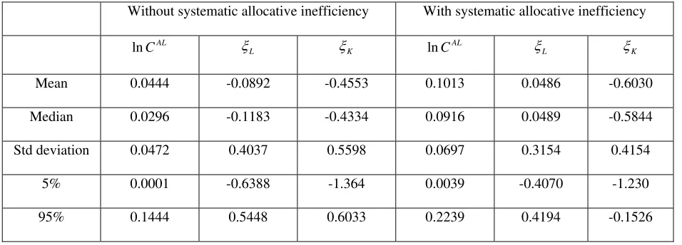
Next we report (in Table 1) the increase in cost due to allocative inefficiency, which is found to be
quite small for both models. The mean (median) values of l is 0.0444 (0.0296), which shows that cost is
increased, on average, by 4.44%. For the top (bottom) 50% of the firms the cost is increased by 2.96% due to input
misallocation. For the bottom 5% of firms, misallocation of inputs increased cost by 14.44%. These figures are much
higher (mean 10.13% and median 9.16%) when firms are allowed to make systematic allocative errors in input-use
decisions. Increase in cost due allocative inefficiency for about half of the firms is more than 9.16%. These figures
for the bottom 5% of the firms are more than 22.39%. Distributions of l (with and without systematic allocative
inefficiency) are plotted in Figure 2. It can be seen that the distribution of without systematic allocative
inefficiency is very tight compared to the one that allows systematic allocative inefficiency. Since these firms were
regulated, then from a static optimization point of view it is expected that inputs, especially capital, won’t be used
optimally (the Averch-Johnson hypothesis). Thus the results from the model that ignores systematic allocative
inefficiency are likely to be biased. This finding accords with the Monte Carlo results in Kumbhakar and Wang
(2005).
ln AL, C
nCAL
n AL C
ln AL C
Results from the models with both technical and allocative inefficiency are reported in Table 2. Increase in
cost due to technical inefficiency, on average, is 9.07% to 9.94% depending on whether or not systematic allocative
inefficiency is allowed. For about half of the firms, the increase in cost due to technical inefficiency is around 8%,
irrespective of whether allocative inefficiency is systematic or not. However, the increase in cost due to allocative
inefficiency, vary widely depending on whether or not allocative inefficiency is assumed to be systematic.
For example, compared to the model without systematic allocative inefficiency it can be seen that the estimated value
of in the model with systematic allocative inefficiency is more than twice (the median values are 8.46% and
3.8%, respectively). In both models we find overuse of capital and labor (relative to fuel), although the degree of such
overuse is more pronounced in the model that allows systematic allocative inefficiency. This is one of the reasons
why is more than double in the model that allows systematic allocative inefficiency. Further insight can be ln AL,
C
lnCAL
obtained from the plots of l in Figure 3. It is clear that distributions of l are much tighter when systematic
allocative inefficiency is not allowed.
nCAL nCAL
Now we examine the returns to scale results, reported in Table 3 and Figure 4. In fact, we report cost
elasticity with respect to output, (which is the reciprocal of returns to scale). Scale economies
(SCE) can then be defined as , which shows economies (diseconomies) of scale if SCE is positive
(negative). We find evidence of scale economies (at the mean/median) from all models. The models with only
allocative inefficiency show smaller scale economies when compared to those with both technical and allocative
inefficiency (evaluated at the mean/median). Figure 4 shows plots of from all four models. Percentage of firms
with scale economies ( ) varies depending on the model. For example, about 94% of the firms in the models
with both technical and with or without allocative inefficiency were operating with economies of scale. However, if
one assumes that firms were operating fully efficiently (technically), then these percentages drop dramatically. For
example, only 62.6% of firms showed economies of scale in the model that allows systematic allocative inefficiency.
On the other hand, the percentage of firms with economies of scale increased to 82.9% if one makes the assumption
that firms were operating without systematic allocative inefficiency. Systematic allocative inefficiency matters more
in the model with no technical inefficiency so far as the estimates of scale economies are concerned. However, all the
models predict the presence of substantial unexploited scale economies, which is also found by Christensen and
Greene (1976). However, these results are in contrast to those reported in Kumbhakar and Wang (2006) who used the
more recent data and found no evidence of substantial scale economies. This is not surprising because the average
size of firms has increased over time to exploit scale economies.
0
ln / ln , CQ
E = ∂ C ∂ q
1 CQ SCE= −E
CQ E
1 CQ E <
Since the Christensen and Greene formulation comes closer to our model with no technical and systematic
allocative inefficiency (Model 1), we compare scale economies derived from these two models. Note that the error
terms in the cost share equations in the Christensen and Greene model have no economic interpretation while in our
model these error terms ( )η are functions of allocative inefficiency ( )ξ . The summary statistics of cost elasticity
from the Christensen and Greene model (Model 5) are reported in the last column of Table 3. A comparison of these
numbers with those from Model 1 shows that estimates are underestimated (SCE are biased upward) in Model 5.
For example, the mean (median) SCE in Model 5 is 0.11 (0.090) whereas in Model 1 it is 0.084 (0.062). CQ
It is often argued that since the data is from the 1970s, the empirical results are not relevant to the electric
utility industry of today. Comparing our results to those that used the recent data (for example, Kumbhakar and
Wang (2006)), we find that efficiency results (both technical and allocative) are in fact qualitatively similar.
However, the estimates of returns to scale are found to be different. While the industry was mostly operating under
increasing returns to scale, no scale economies are found in the recent years. Our finding that most of the firms were
operating under increasing returns to scale is consistent with the findings of Christensen and Greene (1976). That is,
the inclusion of technical and allocative inefficiencies in the Christensen and Greene model did not change their main
result that most of the firms experienced scale economies (although the scale economies results are overestimated). In
general, other results of our models such as own and cross-elasticities of substitution are found to be in agreement
with those reported in Christensen and Greene7.
4.2 Firm-level IT productivity data
We also apply the proposed technique to another very different type of data set that is used by Brynjolfsson
and Hitt (2003) to measure computer (IT) productivity. Since our objective is to apply the cost system approach, we
focused on a single cross-section of 518 firms for the year 1994. The output variable is value added (Q) and the three
variable inputs are: ordinary capital stock (K), computer (IT) capital stock (C), and labor (L). The total cost is the sum
of ordinary capital, computer capital, and labor cost. The details on the definition and construction of these variables
can be found in Brynjolfsson and Hitt (2003). To conserve space we discuss the main results from this data, viz.,
from the models with and without systematic allocative inefficiency.8 In both models price of ordinary capital is used
as a numeraire to impose homogeneity (of degree one) restrictions. Thus, our estimates of allocative inefficiency in
labor and IT capital (ξLand ξC) are relative to ordinary capital. The mean values of ξLand ξCare found to be
positive, which means that labor and IT capital are underused relative to ordinary capital. Alternatively, ordinary
capital is overused relative to both IT capital and labor. It can be seen from the distributions of ξC and ξL (Figures
7 To conserve space, we do not report these results. Details can be obtained from the authors upon request.
5a and 5b) that IT capital under-use (relative to capital) is much less than that of labor. The spread of ξLis quite large
in both models with and without systematic allocative inefficiency.
Since misallocation of inputs increase costs which is what matters most to the producers, it is natural to
examine increase in cost due to allocative inefficiency. The distributions of percentage increase in cost due to
allocative inefficiency for both models (with and without systematic allocative inefficiency) are reported in Figure 8.
On average, cost due to allocative inefficiency, ln CAL, is increased by 6.2% (9.8%) in the model without (with)
systematic allocative inefficiency. The median values of ln CAL in these models are 6.8% and 9.7%, respectively.
Thus, distributions of ln CAL in both models are quite symmetric. However, the variation (spread) in ln CAL in the
model with systematic allocative inefficiency is more pronounced.
Next we examine costs of technical inefficiency (which is the same as input-oriented technical inefficiency),
u. The distribution of u is plotted in Figure 7 for both models. On average, technical inefficiency increased cost by 7.12% (5.81%) in the models without (with) systematic allocative inefficiency. The high mean value of technical
inefficiency in the model without systematic allocative inefficiency is due to the fact that the distribution is highly
skewed to the right and technical inefficiency of several firms is found to be quite high. The median values of
technical inefficiency in both models are quite low in both models (1.54% vs. 1.64%).
Finally, we report cost elasticities, , in Figure 6. From the estimates of we can obtain the measure
of scale economies (SCE) which is , and returns to scale which is the reciprocal of . It can be seen
from Figure 6 that almost all these firms enjoyed economies of scale (operated under increasing returns to scale) in
the model without systematic allocative inefficiency. The mean value of SCE is 0.0736 and is significantly different
from zero. On the other hand, in the model with systematic allocative inefficiency, the mean value of SCE is 0.046.
Finally, the mean value of SCE is reduced to 0.036 when one assumes the firms to be both technically and
allocatively efficient. A closer look at the distribution of shows that although the magnitude of scale economies
is smaller in the model with systematic allocative inefficiency, RTS is found to be greater than unity for about 90% of
the firms. In summary, we find evidence of economies of scale for most of the firms regardless of which model is
used. The distributions of for both models are almost symmetric, and their spreads are quite similar. CQ
E ECQ
1 CQ
SCE= −E ECQ
CQ E
5. Conclusions
In this paper we build on the work of Kumbhakar (1997) and developed an exact maximum likelihood
method for his postulated cost system which models technical and allocative inefficiencies in a theoretically
consistent way. In essence, this methodology permitted us to estimate jointly the cost function parameters as well as
increased cost due to each inefficiency component using cross-sectional data. Our approach solves the long standing
Greene problem, which is associated with estimation of a flexible cost system in the presence of both technical and
allocative inefficiency. We illustrated the working of our model first with only allocative and then both technical and
allocative inefficiencies. The Christensen and Greene (1976) electric utility data are used to estimate the parameters
of our models. We found that costs of technical and allocative inefficiency are sensitive to whether one assumes only
allocative or both technical and allocative inefficiency. The same conclusion is reached for the estimates of returns to
scale. Comparing our results with those that use a much more recent data, we find that efficiency results (both
technical and allocative) are qualitatively similar, but the returns to scale are not.
Our second application used cross-sectional data on 518 large U.S. firms taken from the Brynjolfsson and
Hitt (2003) data. In this data we found that costs of allocative inefficiency are somewhat sensitive to whether or not
allocative inefficiency is assumed to be symmetric. Finally, we found evidence of scale economies in both models,
although it is found to be more pronounced in the model without systematic allocative inefficiency.
References
Bauer, P.W., 1990, Recent Developments in the Econometric Estimation of Frontiers, Journal of Econometrics 46, 39-56.
Brynjolfsson, Erik and Lorin M. Hitt, 2003, Computing Productivity: Firm-Level Evidence, Review of Economics and Statistics 85, 793-808.
Christensen, L. R., and W.H. Greene, 1976, Economies of Scale in U. S. Electric Power Generation, Journal of Political Economy 84, 655-76.
Farrell, M. J., 1957, The Measurement of Productive Efficiency, Journal of the Royal Statistical Society, Series A, 120, 253-81.
Greene, W.H., 1980, On the Estimation of a Flexible Frontier Production Model, Journal of Econometrics 13:1, 101-15.
Kumbhakar, S.C. and C.A.K Lovell, 2000, Stochastic Frontier Analysis (Cambridge University Press, New York). Kumbhakar, S.C., and E.G Tsionas, 2005, The Joint Measurement of Technical and Allocative Inefficiencies: An
Application of Bayesian Inference in Nonlinear Random-Effects Models, Journal of American Statistical Association 100, 736-747.
Kumbhakar, Subal C, and Wang, Hung-Jen, 2006, Estimation of Technical and Allocative Inefficiency in a Stochastic Frontier Production Model: A System Approach, Journal of Econometrics (forthcoming).
Kumbhakar, Subal C, and Wang, Hung-Jen, 2005, Pitfalls in the Estimation of Cost Function Ignoring Allocative Inefficiency: A Monte Carlo Analysis, Journal of Econometrics (forthcoming).
McElroy, M., 1987, Additive General Error Models for Production, Cost, and Derived Demand or Share System, Journal of Political Economy 95, 738-57.
Table 1: Only allocative inefficiency
Without systematic allocative inefficiency With systematic allocative inefficiency
lnCAL
L
ξ ξK ln
AL
C ξL ξK
Mean 0.0444 -0.0892 -0.4553 0.1013 0.0486 -0.6030
Median 0.0296 -0.1183 -0.4334 0.0916 0.0489 -0.5844
Std deviation 0.0472 0.4037 0.5598 0.0697 0.3154 0.4154
5% 0.0001 -0.6388 -1.364 0.0039 -0.4070 -1.230
95% 0.1444 0.5448 0.6033 0.2239 0.4194 -0.1526
Table 2: Both technical and allocative inefficiency
Without systematic allocative inefficiency With systematic allocative inefficiency
u lnCAL
L
ξ ξK u ln
AL
C ξL ξK
Mean 0.0994 0.0569 -0.0884 -0.5324 0.0907 0.1052 -0.1465 -0.8078
Median 0.0882 0.0380 -0.1184 -0.5359 0.0784 0.0846 -0.2029 -0.7929
Std. dev. 0.0533 0.0582 0.4009 0.5731 0.0504 0.0874 0.4145 0.6331
5% 0.0305 0.0005 -0.7264 -1.472 0.0321 0.0052 -0.7074 -1.8190
[image:21.612.62.544.515.709.2]95% 0.2057 0.0005 0.5890 0.2178 0.2046 0.2854 0.4915 0.0713
Table 3: Output cost elasticity
Only allocative inefficiency Both technical and allocative inefficiency
without systematic
Model 1
with systematic
Model 2
without systematic
Model 3
with systematic
Model 4 Model 5
Mean 0.9155 0.9595 0.8870 0.8898 0.8866
Median 0.9378 0.9799 0.9078 0.9099 0.9066
Std deviation 0.1003 0.0970 0.0967 0.0954 0.0929
5% 0.6217 0.6699 0.6051 0.6115 0.6146
Appendix: Existence and uniqueness of solution to the system of equations Theorem: If
(A1) the actual share a 0 for all , i
S > i∈ =Z {1,..., }J
(A2) for every i∈Z, we have (β ≠ij 0 for some j∈Z), where βij represents the second-order translog coefficients with respect to prices,
(A3) jk 0 j
β
∈ =
∑
Z , and
(A4) 0j 1, j
S
∈ =
∑
Z
then (i) there exists a solution of ξin the system of equations in (14), and (ii) the solution is unique.
Proof: Before proving the existence and uniqueness, we note that the condition in (A1) follows from the definition of cost shares, while that in (A2) is necessary for flexibility of the translog cost function. Finally, the conditions (A3) and (A4) follow from homogeneity (of degree one in input prices) of the cost function.
(i) Existence.
The system in (14) is of the form aexp( ) 0
j j j jk k
k
S ξ G S β ξ
∈
= + ∑
Z , j∈Z
κ = ξ j∈Z κ = +ξ + j
. Note that here we are considering
the system in which the homogeneity restrictions are not directly imposed by expressing all prices and cost relative to
one input price. Let aexp( ) , , so that ,
j Sj j G ln ln ln
a
j Sj j G ∈Z. Then the system in (14) can be written in the form
0 ln a ln ln 0 ln a ln
j j jk k jk k jk j jk k jk k
k k k k k
S S G S S
κ β β κ β β β κ
∈ ∈ ∈ ∈ ∈
= − ∑ + ∑ − ∑ = −∑ + ∑
Z Z Z Z Z , j∈Z. (A.1)
such that . Then , the unit simplex in . Write the residual from the cost
share system (3) as 1 j j κ ∈ = ∑
Z { |
n j j
κ κ + κ
∈
∈ ≡ ∈\ ∑ =
Z
S 1}
k k
f κ κ S S
n
\
0
( ) ln a ln
j j j βjk k βjk κk
∈ ∈
= − + ∑ − ∑
Z Z , j∈Z. (A.2)
Define the mapping
2
2
( ) ( )
1 ( )
j j j k k f g f κ κ κ κ ∈ + = + ∑ Z
j∈Z
*
, .
Clearly, , i.e., it maps S into itself and is continuous. By Brouwer's fixed point theorem, there exists a
such that , which implies that :
g S S→
*
κ ∈S g(κ*)=κ
* 2 * * 2
( ) ( )
j j k
k
f κ κ f κ
∈
= ∑
Z , j∈Z.
Multiplying both sides by ( *) and summing over we obtain j
* 3 * * * 2
( ) ( ) ( )
j j j k
j j k
f κ κ f κ f κ
∈ = ∈ ∈
∑ ∑ ∑
Z Z Z .
Suppose ( *) 0 for all but j
f κ = j≠l fl(κ ≠*) 0. Then the above equation implies
* 3 * * 3
( ) ( )
l l l
f κ =κ f κ , which gives . Write
* 0
l
κ = * aexp( )
l Sl l
κ = ξ* . By assumption (A1) since * 0
l
κ = we have *
l
ξ = −∞. For by (A.2) we obtain
for some provided assumption (A2) holds. Now,
* 0 l κ = * ( ) j
f κ = ±∞ j∈Z
* *
* *
* 2
( ) ( )
1 ( )
l l l l l f g f κ κ κ κ κ + = = + 2
. Although * 0
l
κ = ,
the limit of the right hand side expression as (and therefore as ) is equal to one, a
contradiction since is continuous. Therefore, we conclude that at the fixed point
* 0
l
κ → ( * 2)
l
f κ → +∞ ( )
l
g κ κ* we must have ( *) 0
j f κ = for all j∈Z which means that κ* represents a solution.
(ii) Uniqueness.
Suppose { }ξj and { }ϕj are distinct solutions. Therefore they must satisfy
0
exp( ) a
j j j jk
k
S ξ G S β ξk
∈ = + ∑ Z 0 exp( ) a
j j j jk
k
S ϕ G S β ϕk
∈
= + ∑
Z , (A.3) for all j∈Z, and they also satisfy the following equality
exp( ) exp( ) 1
a a
j j j j
j j
S ξ S
∈ = ∈
∑ ∑
Z Z ϕ =
k
. (A.4)
Define εk =ξ ϕk− so that we have exp( )[exp( 1)] a
j j j jk
k
S ϕ ε β εk
∈
− = ∑
Z . Let exp( )
a j Sj ϕj
Λ = and notice that
j
exp(εj− ≥1) ε to obtain jk k j j k
β ε
∈ ≥ Λ
∑
Z ε . This system can be written in the form [B−diag( )]Λ ε≥0. Now choose a vector such that c cε′ <0, which is always possible provided not all the εjs are zero (a fact that we have to accept
since we have assumed the existence of two different solutions). By applying the Farkas’ lemma we obtain that since
the above system has a solution, the system [B−diag( )]Λ ε =c, ε≥0 must have no solution. Therefore, there exists
no nonnegative vector ε to satisfy jk k j j j k
c
β ε ε
∈ = Λ +
∑
Z . We set ε =j w for all j so we know that there exists no nonnegative w to satisfy . We will obtain an obvious contradiction provided we can show that the
inequality
j
c = − Λw j
0
cε′ < is satisfied. But 2 0 since the
j j j
j j
cε cε w
∈ ∈
′ = ∑ = −∑ Λ
] ] < Λjs are positive. The contradiction shows