Using
R
and Bioconductor for proteomics data analysis
Laurent Gatto1,∗, Andy Christoforou
Cambridge Centre for Proteomics, Department of Biochemistry University of Cambridge, Tennis Court Road, Cambridge, CB2 1QR, UK
Abstract
This review presents howR, the popular statistical environment and programming language,
can be used in the frame of proteomics data analysis. A short introduction toRis given, with
special emphasis on some of the features that make R and its add-on packages a premium
software for sound and reproducible data analysis. The reader is also advised on how to find
relevant R software for proteomics. Several use cases are then presented, illustrating data
input/output, quality control, quantitative proteomics and data analysis. Detailed code and additional links to extensive documentation are available in the freely available companion
packageRforProteomics.
Keywords: software, mass spectrometry, quantitative proteomics, data analysis, statistics,
quality control
1. Introduction
1
Proteomics is evolving at a rapid pace [1] and updates in technologies and instruments
2
applied to the study of bio-molecules, such as proteins or metabolites, require proper
com-3
putational infrastructure [2]. A broad diversity of complementary tools for data processing,
4
management, visualisation and analysis have already been offered to the community and
5
reviewed elsewhere [3,4]. The work presented here focuses on a particular type of software,
6
namely R [5], and the add-onpackages that enable extension in its functionality and scope,
7
and their usefulness to the analysis of proteomics data.
8
∗Corresponding author
Email addresses: [email protected](Laurent Gatto),[email protected](Andy Christoforou)
Ris an open source statistical programming language and environment, originally created
9
by Ross Ihaka and Robert Gentleman [6] at the University of Auckland and, since the
mid-10
1997, developed and maintained by the R-core group. Originally utilised in an academic
11
environment for statistical analysis, it is now widely used in public and private sector in a
12
broad range of fields [7], including computational biology and bioinformatics. The success
13
of R can be attributed to several features including flexibility, a substantial collection of
14
good statistical algorithms and high-quality numerical routines, the ability to easily model
15
and handle data, numerous documentation, cross-platform compatibility, a well designed
16
extension system and excellent visualisation capabilities to list some of the more obvious
17
ones [8]. These are some of the requirements that need to be fulfilled to tackle the complexity
18
and high-dimensionality of modern biology.
19
The focus of Ritself is and remains centred around statistics and data analysis.
Function-20
ality can however be extended through third-party packages, which bundle a coherent set of
21
functions, documentation and data to address a specific problem and/or data type of
inter-22
est. The Bioconductor project2 [9], initiated by Robert Gentleman, has a specific focus on
23
computational biology and bioinformatics and represents a central repository for hundreds
24
of software, data and annotation packages dedicated to the analysis and comprehension of
25
high-throughput biological data, and promoting open source, coordinated, cooperative and
26
open development of interoperable tools. The development and distribution of new packages
27
is a very dynamic and important aspect of the R software itself. Adherence to good
devel-28
opment practice is crucial and enforced by the R package development pipeline through a
29
built-in checking mechanism, ensuring, among other things, proper package installation and
30
loading, package structure, code validity and correct documentation. In addition, package
31
development also provides multiple opportunities for unit and integration testing as well as
32
reproducible research [10, 11, 12, 13, 14] through the mechanism of literate programming
33
[15] and Sweave [16] or knitr [17] vignettes, which is crucially important from a scientific
34
perspective.
35
Packages can be submitted to the main central repository, the ComprehensiveR Archive
36
Network (CRAN) or to Bioconductor, which provides its own repository, to assure tighter
37
software interoperation. In addition, any developer can easily set up private or public
38
CRAN-style systems. Software management can become a tedious task when thousands of
39
packages are distributed, many of which depend on each other and interoperate in complete
40
pipelines. In R, this has been solved by providing dedicated package repositories as well as
41
straightforward installation and updating mechanisms.
42
Most importantly, R and many packages are regarded as quality software [18]. They are
43
aimed at users who want to explore and comprehend complex data for which there is often
44
no predefined recipe. It is also a research tool to tackle new questions in innovative ways.
45
The Bioconductor project, for example, has had a substantial impact on the field of
microar-46
rays through multi-disciplinary and cooperative method development and implementation,
47
paving best practises for the current development of state-of-the-art high throughput
ge-48
nomics data analysis and comprehension. With respect to R’s contribution to other areas
49
of bioinformatics and computational biology, it has also a lot to offer to proteomics.
Biolo-50
gists and proteomicists can gain immensely from autonomous data exploration and analysis.
51
Bioinformaticians working in computational proteomics can useR and specialised packages
52
as an independent analysis and research framework or employ them to complement existing
53
pipelines.
54
This manuscript presents a brief overview of some applications of the R software to
55
the analysis of MS-based quantitative proteomics data. We will review compliance of R
56
with open proteomics data standards, input/output capabilities, quantitation pipelines for
57
label-free and labelled quantitation, quality control, quantitative data analysis and relevant
58
annotation infrastructure. The review is accompanied by a package, RforProteomics, that
59
provides the code to install a selection of relevant tools to reproduce and adapt the examples
60
described below. Installation instruction are provided on the package’s web page3. Once
61
installed, the package is loaded with the library function as shown below, to make its
62
3
functionality available.
63
> library("RforProteomics")
This is the ’RforProteomics’ version 1.0.1. Run ’RforProteomics()’ in R or visit
’http://lgatto.github.com/RforProteomics/’ to get started.
2. Using R in proteomics
64
2.1. Finding relevant software
65
R is a very dynamic ecosystem [19, 20] – yearly R and bi-annual Bioconductor releases,
66
exponentially growing number of available packages [21], numerous active mailing lists and a
67
community of hundreds of thousands of active users and developers in private and corporate
68
environment [7]. There are currently thousands of packages available through the official
69
repositories, and new packages are published, discontinued or replaced by new, more
elabo-70
rate alternatives on a daily basis. Providing an up-to-date and exhaustive list of packages
71
is unachievable, even for a specified area of interest like proteomics, and would undoubtedly
72
be out-dated too quickly to be useful. Dedicated pages are available however, that allow one
73
to obtain an overview of some of the available packages in a specific area. CRAN maintains
74
topic task views4, which are curated and maintained by experts. Each view provides a
sum-75
mary and some guidance on some of the growing number of CRAN packages that are useful
76
for a certain topic. As of this writing, the Chemometrics and Computational Physics view
77
features a total of 67 packages, some of which are dedicated to mass spectrometry and will
78
be described later. The Bioconductor project provides a set of dedicated keywords to
cate-79
gorise packages, calledbiocViews, that can be explored interactively5. For proteomics, most
80
relevant candidates are MassSpectrometry (in the Software/AssayTechnology view with 21
81
packages) andProteomics (in the Software/BiologicalDomain view, 35 packages), although
82
numerous data analysis and annotation packages in other categories provide invaluable
sup-83
port, some of which will also be demonstrated below.
84
4http://cran.r-project.org/web/views/
5
2.2. Getting suitable data
85
Software development, evaluation and demonstration can not be envisioned without
ap-86
propriate data. AlthoughRpackages most often focus on software functionality, packages are
87
also used to distribute experimental and annotation data, displayed in the AnnotationData
88
and ExperimentData biocViews. A specific MassSpectrometryData category, currently
of-89
fering 5 packages, is dedicated for experimental data of interest here. Software packages
90
often also distribute small data sets for illustration, demonstration and code testing.
91
To exemplify some of the pipelines in this publication, we will make use of a larger,
92
public data set, available from the ProteomeXchange6[22] ProteomeCentral repository (data
93
PXD0000017). In this TMT 6-plex [23] experiment, four exogenous proteins were spiked
94
into an equimolar Erwinia carotovora lysate with varying proportions in each channel of
95
quantitation; yeast enolase (ENO) at 10:5:2.5:1:2.5:10, bovine serum albumin (BSA) at
96
1:2.5:5:10:5:1, rabbit glycogen phosphorylase (PHO) at 2:2:2:2:1:1 and bovin cytochrome C
97
(CYT) at 1:1:1:1:1:2. Proteins were then digested, differentially labelled with TMT reagents,
98
fractionated by reverse phase nanoflow UPLC (nanoACQUITY, Waters), and analysed on
99
an LTQ Orbitrap Velos mass spectrometer (Thermo Scientific). Files in multiple format
100
will be used to illustrate the input/output capabilities that are available to the proteomics
101
audience. The companion package provides dedicated functions to directly download the
102
data.
103
2.3. Proteomics standards and MS data input-output
104
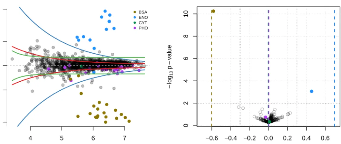
Proteomics is a very diverse field in terms of applications, experimental designs and file
105
formats. When dealing with a wide range of data, flexibility is often key; this is particularly
106
relevant for the R environment, which can be used for many different purposes and data
107
types. Raw mass spectrometry data comes in many different formats. While closed
vendor-108
specific binary formats are less interesting due to their limited scope, several research groups
109
as well as the HUPO Proteomics Standards Initiative (PSI) have developed open XML-based
110
6http://www.proteomexchange.org/
7Data DOI:
standards, formats and libraries to facilitate the development of vendor-agnostic tools and
111
analysis pipeline. This functionality is available through the mzR package [24, 25], that
112
provides a unified interface to the mzData [26], mzXML [27], mzML [28] as well as netCDF
113
formats. TheopenMSfilefunction opens a connection to any of these file types and enables
114
to query instrument information and raw data in a consistent way. It is generally used by
115
experienced users or developers who require maximal flexibility. For instance, mzR is used
116
byxcms [29, 30], TargetSearch[31] and MSnbase[32] for interaction with raw data.
117
Other packages provide higher level interfaces to raw data, modelled as computational
118
data containers that store data and meta-data while assuring internal coherence. Such
119
classes come with a set of associated methods, that allow the application of predefined
120
actions on class instances, also calledobjects, such as accessing specific pieces of information,
121
modifying parts of the data or producing relevant graphical representation of the data. The
122
MSnExporxcmsRawclasses, defined in theMSnbaseandxcmspackages respectively, represent
123
experiments as a collection of annotated spectra, with the aim of removing the burden of
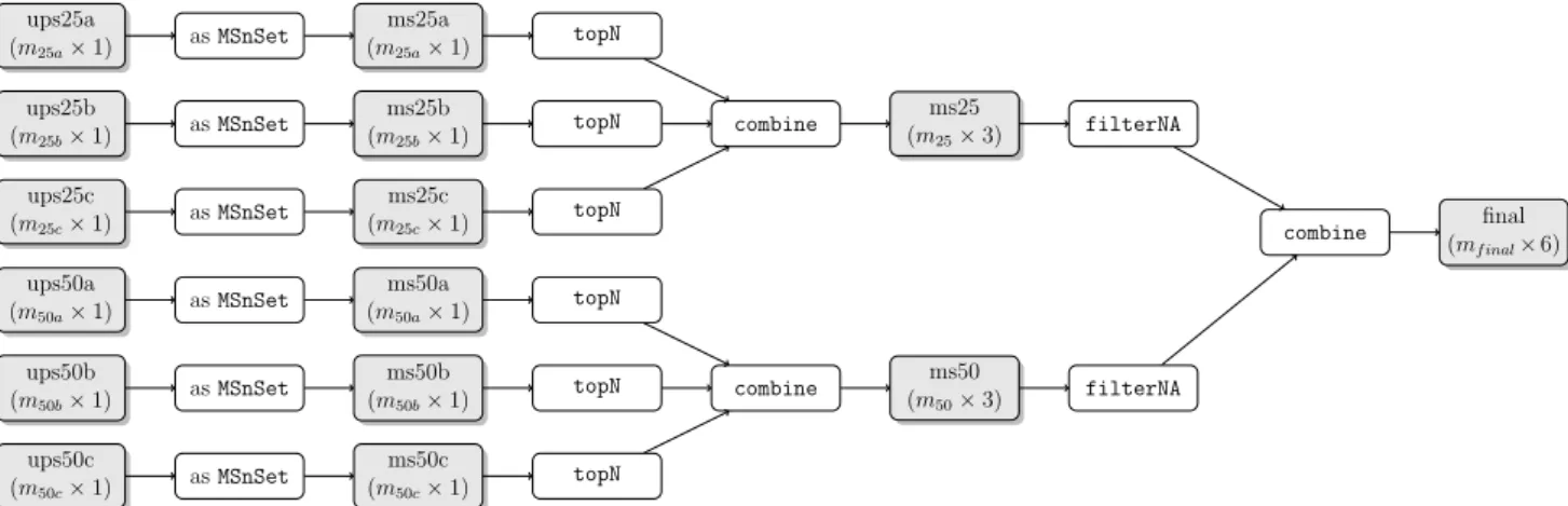
124
users to manipulate the complex data by bundling it in specialised classes with an
easy-to-125
use and well documented interface, the associated methods, to streamline the most common
126
tasks. The example raw file used below, available from the MSnbase package, is an iTRAQ
127
4-plex [33] experiment. It is read into R and converted into an MSnExp object using the
128
readMSData function. This specific data structure allows the spectra to be stored along
129
with associated meta data and enables easy manipulation of the complete annotated data
130
set. The last line displays a summary of the data in the R console and figure 1 illustrates
131
some of the raw data plotting functionality applicable to an MSnExp instance (left) or an
132
individual spectrum (right).
133
This first command finds the location of the test data file.
134
> mzXML <- dir(system.file(package = "MSnbase", dir = "extdata"), + full.name = TRUE, pattern = "mzXML$")
We then proceed by reading the mzXML file and create an MSnExp object.
> rawms <- readMSData(mzXML, verbose = FALSE)
Finally, we show a summary of the contents of the data object.
136
> rawms
Object of class "MSnExp"
Object size in memory: 0.2 Mb
Spectra data
-MS level(s): 2
Number of MS1 acquisitions: 1
Number of MSn scans: 5
Number of precursor ions: 5
4 unique MZs
Precursor MZ's: 437.8 - 716.34 MSn M/Z range: 100 2017
MSn retention times: 25:1 - 25:2 minutes
Processing information
-Data loaded: Tue Apr 9 22:10:44 2013
MSnbase version: 1.9.1
- - - Meta data
-phenoData
rowNames: 1
varLabels: sampleNames fileNumbers
varMetadata: labelDescription Loaded from: dummyiTRAQ.mzXML protocolData: none featureData featureNames: X1.1 X2.1 ... X5.1 (5 total) fvarLabels: spectrum fvarMetadata: labelDescription
experimentData: use 'experimentData(object)'
[Fig. 1 about here.]
137
The mgf file format is also supported, for reading through the function readMgfData,
138
which encapsulates the peak list data into MSnExp objects as above, and for writing such
139
objects to a file through the writeMgfData. Other input/output facilities for quantified
140
data will be presented in the next section.
Standard formats for identification data are not yet systematically supported. It is
142
however possible to import such information into R , using existing R data import/export
143
infrastructure. For example, the XML package [34] allows one to parse arbitrary xml files
144
based on their schema definition. Support for mzIdentML, mzQuantML and possible other
145
community supported formats will be added to the mzR package.
146
2.4. Data processing and quantitation
147
Quantitation has become an essential part of proteomics, and several alternatives are
148
available inR for label-free and labelled approaches. In this section, we will present
quanti-149
tation functionality and associated raw data processing capabilities.
150
2.4.1. Label-free quantitation
151
Several packages provide functionality that can be applied to the analysis of label-free
152
MS data. Although its first scope is the study of metabolites,xcmsis a mature package that
153
provides a complete pipeline for preprocessing LC/MS data for relative quantitation and
154
data visualisation [35, 36]. A typical xcms work flow implements peak extraction, filtering,
155
retention time correction and matching across samples. The package is very versatile,
featur-156
ing, for example, several peak picking methods, including some applying continuous wavelet
157
transformation (CWT) [37, 38]. The pipeline offers a complete framework to support data
158
analysis and visualisation of chromatograms and peaks to be deemed to be differentially
159
expressed. On-line help is available though a dedicated forum8.
160
MALDIquant [39] also provides a complete analysis pipeline for MALDI-TOF and other
161
label-free MS data. Its distinctive features include baseline subtraction using the SNIP
162
algorithm [40], peak alignment using warping functions, handling of replicated
measure-163
ments as well as supporting spectra with different resolutions. Figure2illustrates spectrum
164
preprocessing and peak detection steps.
165
[Fig. 2 about here.]
166
8
synapter is a package [41] dedicated to the re-analysis of data independent MSE data
167
[42,43], acquired on Waters Synapt instruments . It implements robust data filtering
strate-168
gies, calculating and using peptide identification reliability statistics, peptide-to-protein
am-169
biguity and mass accuracy. It then models retention time deviations between reliable sets
170
of peptides in different runs and transfer identification across acquisitions to increase the
171
overall peptide and protein coverage in full experiments through an easy-to-use interface.
172
As illustrated in section 2.6, it interoperates well with MSnbase to take advantage of the
173
existing data structure and offers a complete analysis pipeline.
174
Finally, packages that implement MS2 data processing, like MSnbaseand isobar[44] (see
175
section 2.4.2), also support spectral counting once identification data is available. In
addi-176
tion,isobarallows one to perform emPAI [45] and distributed normalised spectral abundance
177
factor (dNSAF) [46] quantitation.
178
2.4.2. Labelled quantitation
179
Pipelines for labelled MS2 quantitation, using isobaric tagging reagents such as iTRAQ
180
and TMT are available in the isobar and MSnbase packages. The code chunk below, taken
181
from MSnbase, illustrates how to quantify the iTRAQ reporter peaks from the rawms data
182
instance read in section 2.3. The quantify function returns another data container, an
183
MSnSet, specialised for storing quantitative data and associated meta data. Reporter
impu-184
rity correction can then be applied using the purityCorrect. The isobar package imports
185
centroided peak data identification data from mgf and text spread sheet files or converts
186
MSnSet instances to create its own IBSpectra containers for further isotope impurity
cor-187
rection, normalisation and differential expression analysis (section 2.6).
188
Below, we perform quantitation of the rawMSnExpdata using the iTRAQ 4-plex reporters
189
ions to create a new MSnSet object containing the quantitative data.
190
> qnt <- quantify(rawms, reporters = iTRAQ4, verbose = FALSE)
In the following code chunk, we first define the reporter tag impurities as reporter by the
191
manufacturer, apply the correction and display a summary of the resultingMSnSet instance.
> impurities <- matrix(c(0.929, 0.059, 0.002, 0.000, + 0.020, 0.923, 0.056, 0.001, + 0.000, 0.030, 0.924, 0.045, + 0.000, 0.001, 0.040, 0.923), + nrow=4) > qnt <- purityCorrect(qnt, impurities) > qnt
MSnSet (storageMode: lockedEnvironment)
assayData: 5 features, 4 samples
element names: exprs
protocolData: none
phenoData
sampleNames: iTRAQ4.114 iTRAQ4.115 iTRAQ4.116
iTRAQ4.117
varLabels: mz reporters
varMetadata: labelDescription
featureData
featureNames: X1.1 X2.1 ... X5.1 (5 total)
fvarLabels: spectrum file ... collision.energy (12
total)
fvarMetadata: labelDescription
experimentData: use 'experimentData(object)' Annotation: No annotation
Processing information
-Data loaded: Tue Apr 9 22:10:44 2013
iTRAQ4 quantification by trapezoidation: Tue Apr 9 22:10:49 2013
Purity corrected: Tue Apr 9 23:44:45 2013
MSnbase version: 1.9.1
Once spectrum-level data is produced and stored in the specialised containers with
pep-193
tide identification and protein inference meta data, it can be visualised (see figure 3) and
194
combined into peptide- and protein-level quantitation data.
195
[Fig. 3 about here.]
196
Data analysis capabilities, including data normalisation and statistical procedures, are
197
well known strengths of the R software. It is therefore important to provide support for
198
the exchange of quantitative data. The newly developedmzTab9 file, that aims at
facilitat-199
9
ing proteomics and metabolomics data dissemination to a wider audience through familiar
200
spreadsheet-based format, can also be incorporated and exported using thereadMzTabData
201
andwriteMzTabData functions. It is of course also possible to import quantitation data
ex-202
ported by third party applications to spread sheet formats. The most general way to import
203
such data is using the read.table function. Specialised alternatives exist, to produce data
204
structures, like MSnSets. The readMSnSet function, for instance, can import quantitation
205
data, feature meta data and sample annotation from spread sheets and create fully-fledged
206
MSnSet instances.
207
Additional packages provide specialised functionalities relevant to data processing. IPPD
208
[47] uses template matching to deconvolute peak patterns in individual raw spectra or
com-209
plete experiments. Rdisop [48, 49] is designed to determine the formula of ions based on
210
their exact mass or isotope pattern and can, reciprocally, estimate these from a formula.
211
OrgMassSpecR [50] has similar capabilities including specific functions to process peptide
212
and protein data: it allows the user, for example, to digest proteins, fragment peptides and
213
estimate peptide isotopic distributions modified peptides with, for example, variable 15N
214
incorporation rates. In the RforProteomics documentation, we demonstrate how to assess
215
protein abundance of the yeast enolase spike present across the 6PXD000001 channels using
216
OrgMassSpecR’s Digest function and observe that, allowing for one missed cleavage, we
217
observe 13 out of 79 peptides with length greater than 7 residues (corresponding to the
218
shortest identified ENO peptide), as illustrated in figure 4. The LATEX code producing the
219
alignment for the figure has been generated automatically, from within R, using the protein
220
sequence and observed peptide sequences and TEXshade [51].
221
[Fig. 4 about here.]
222
2.5. Quality control
223
Data quality is a concern in any experimental science, but the high throughput nature
224
of modern omics technologies, including proteomics [52, 53], requires the development of
225
specific data exploration techniques to highlight specific patterns in data. Examination of
complex data is greatly facilitated by well structured containers such as those cited above,
227
that enable direct access to a specific set of values. This, in turn, streamlines the
implemen-228
tation of default and robust pipelines that recurrently query the same data to produce the
229
diagnostic plots and metrics. It is however also often necessary to manually explore data
230
specificity, making the availability of data management facilities even more important.
231
In this section, we present 3 quality plots (figure5) that can be used to assess the intrinsic
232
features of the PXD000001 data set at different levels. On the left, the distribution of MS2
233
delta m/z [54] allows the user to assess the relevance of peptide identification; high quality
234
data showm/z differences corresponding to amino acid residue masses rising well above the
235
general noise level in the histogram. One can also observe a peak at 44 Da, corresponding
236
to the mass of a polyethylene glycol (PEG) monomer, a common laboratory contaminant in
237
MS. The middle figure illustrates incomplete dissociation of TMT reporter tags, a technical
238
characteristic of the labelling approach. Incomplete dissociation of the reporter and balance
239
moieties of isobaric tags result in this additional single fragment ion peak, in which the
240
multiple channels of quantitation remain convoluted. The figure illustrates the sum of
241
genuine reporter peaks as a function of incompletely dissociated reporter data. The dotted
242
line corresponds to equal real and lost signal. A linear model has been fitted to the data
243
(blue line), indicating that there is, on average, 100-fold more genuine reporter signal. The
244
heatmap on the right indicates the relevance of our quantitation data at the level of our
245
experiment. Congruent peptide clustering indicates agreement between spike peptides while
246
no significant grouping is detected for the samples.
247
[Fig. 5 about here.]
248
Although the figures above are helpful individually, quality assessment is often most
249
efficient when put into context. Lab-wide monitoring of quality properties and metrics over
250
time to gain experience of average performances and critical thresholds, is the most efficient
251
and valuable application of quality control; the tools presented in this section are one way
252
to automate such a process.
2.6. Data analysis
254
In this section, we will describe data analysis pipelines for two quantitative strategies,
255
namely MSElabel-free and isobaric tagging, using synapter and isobarrespectively.
256
Once quantitation data is obtained, it is often desirable to correct technical biases to
257
improve detection of biologically relevant proteins. The availability of well established
nor-258
malisation algorithms within the Bioconductor project are directly applicable here. The
259
MSnSet object called qnt, created in section 2.4.2 can be normalised using various
meth-260
ods, including quantile normalisation [55] and variance stabilisation [56, 57] using a single
261
normalize command. isobar also has similar functionality, tailored for IBSpectra objects;
262
its normalize method corrects by a factor such that the median intensities in all reporter
263
channels are equal.
264
isobar implements methodology to model variability in the data. We will illustrate this
265
using thePXD000001data to estimate spectra and proteins exhibiting significant differences
266
between channel 127 and 129. As shown on figure 6, experimental noise has been
approxi-267
mated using the NoiseModel function on Erwinia background (red), spiked-in (blue) or all
268
(green) peptides (left) and protein ratios and significance have been computed (using the
269
full noise model) with the estimateRatio function, to call statistically relevant proteins.
270
[Fig. 6 about here.]
271
Data independent MSE acquisition from a Synapt mass spectrometer (Waters) can be
272
efficiently analysed in R using the synapter pipeline, providing a complete and open work
273
flow (figure7) leading to comprehensive data exploration and more reliable results. The test
274
data used for this illustration is a spiked-in set distributed with the synapterdatapackage: 3
275
replicates (labelleda toc) of the Universal Proteomics Standard (UPS1, Sigma) 48 protein
276
mix at 25 fmol and 3 replicates at 50 fmol, in a constantEscherichia coli background. The
277
set of functions insynapterproduce data in a specific data container, calledSynapterobjects,
278
and labelledupson figure 7. They store quantitative data for a set ofm identified peptides
279
for one unique sample. Although at this step, much has been gained in terms of reliability
and number of peptides, we are still far from having interpretable results at this stage. These
281
Synapterobjects can easily be converted intoMSnSetinstances (of dimensionsmi×1, where
282
mi is the number of peptides for the processed sample, labelledms on figure7). Each newly
283
converted MSE data can now be quantified using the top 3 method [42] (or any top n
284
variant) where the intensities of the 3 most intense peptides for each protein are aggregated
285
to estimate protein quantities. Each set of replicates is then combined into two new mi×3
286
MSnSet instances (named ms25 and ms50), one for each set of spike concentration, that are
287
then filtered for missing quantitation, keeping only proteins that have been quantified in at
288
least 2 out of 3 replicates. ms25 and ms50 are finally combined into the final mi ×6 final
289
data, normalised and subjected to a statistical analysis. As illustrated above, it becomes
290
possible to design specific pipelines for any type of experiments using standardised methods
291
and data structures.
292
[Fig. 7 about here.]
293
2.7. MS2 spectra identification
294
A very recent addition to Bioconductor is the rTANDEMpackage [58]. The package
en-295
capsulates the mass spectrometry identification algorithm X!Tandem [59], the software for
296
protein identification by tandem mass spectrometry, inR, making it possible to perform MS2
297
spectra identification within theRenvironment and directly benefit fromR’s data mining
ca-298
pabilities to explore the results. The package includes the X!Tandem source code eliminating
299
independent installation of the search engine. In its most basic form, the package allows to
300
call thetandem(input)function, whereinputis either an object of a dedicated class or the
301
path to a parameter file, as one would executetandem.exe /path/to/input.xmlfrom the
302
command line. The results are, as in the original X!Tandem software, stored in anxml, which
303
can however be imported into R in a straightforward way using the GetResultsFromXML
304
function to subsequently extract the identified peptides and inferred proteins.
305
rTANDEM is currently the only direct R interface to a search engine and is as such of
306
particularly noteworthy. Other alternatives require to execute the spectra identification
outside of Rand import, export it in an appropriate format and subsequently import is into 308 R . 309 2.8. Annotation infrastructure 310
The Bioconductor project provides extensive annotation resources through curated
off-311
line annotation packages, that are updated with every release, or through packages that
312
provide direct on-line access to web-based repositories. The former can be targeted towards
313
specific organisms (e.g. org.Hs.eg.db [60] for Homo sapiens) of systems-level annotation
314
such as gene ontology (the GO.db package [61] to gain access to the Gene Ontology [62]
315
annotation) or gene pathways (thereactome.db [63] interface to the reactome database [64,
316
65]). biomaRt[66,67] is a very flexible solution to build elaborated web queries to dedicated
317
data mart servers. Both approaches have advantages. While on-line queries allow one to
318
obtain the latest up-to-date information, they rely on network availability and immediate
319
reproducibility in less straightforward to control.
320
In theRforProteomicsdocumentation, we demonstrate a use case applying 3
complemen-321
tary alternatives. If one wishes, for example, to extract sub-cellular localisation for a gene
322
of interest, say the human HECW1 gene with Ensembl id ENSG00000002746, it is possible
323
to use (1) the hpar package [68] to query the Human Protein Atlas data [69, 70] or (2) to
324
query the org.Hs.eg.db and GO.db annotations to extract the relevant information or (3)
325
biomaRt to query the Ensembl server. Each alternative reports the same location, namely
326
nucleus and cytoplasm, although this might not be necessarily the case. The hpar results
327
are very specific and manually annotated, specifying that the protein, although observed in
328
the nucleus, has not been observed in the nucleoli. The other generic alternatives provide
329
additional information, including GO evidence codes.
330
To conclude this section, we also refer readers to the rols package [71], which provides
331
on-line access to 85 ontologies through the ontology look-up service [72, 73]. Among those
332
are the PRIDE, PSI-MS (Mass Spectrometry), PSI-MI (Molecular Interaction) PSI-MOD
333
(Protein Modifications), PSI-PAR (Protein Affinity Reagents) and PRO (Protein Ontology)
334
controlled vocabularies to name those specific to proteomics and mass spectrometry.
3. Conclusions
336
We have illustrated data processing and analysis on a set of test and small size data.
337
While real life data sets can be processed on commodity hardware or small servers (see
338
supplementary file of [32] and theMSnbase-demovignette for reports), the sophistication of
339
the biological questions of interest and the increase in throughput of instruments requires
340
software tools to adapt and scale up. R is an interpreted language (although support for
341
byte code compilation is available through thecompilerpackage) and relies in many aspects
342
on a pass-by-value semantics, slowing execution of code compared to compiled languages
343
and pass-by-refence semantics. Fortunately, R’s ability to interoperate with many other
344
languages, including C and C++ [74], allows users to execute computationally demanding
345
tasks while still retaining the flexibility and interactivity of the R environment. Direct
346
support for parallel computing, large memory/out-of-memory data (see for instance
High-347
Performance Computing task view10) and cloud deployment with the Bioconductor Amazon
348
Machine Image11, make it possible to embark on large-scale data processing tasks.
349
Among the brief list of packages that has been reviewed, we have demonstrated
alter-350
native and complementary functionality. Most noteworthy however, is the interoperability
351
of these packages, as illustrated in some of the examples. Generally, no specific effort is
352
expected from developers to explicitly promote interaction among packages (on CRAN for
353
example), and thus it is often the user’s/programmer’s responsibility to implement
interop-354
erability. The Bioconductor project, on the other hand, openly promotes interoperability
355
between packages and reuse of existing infrastructure. The classes for raw and processed
356
data, briefly described in sections 2.3 and 2.4 are adapted from and compatible with
ex-357
isting implementations for transcriptomics data, widely used in many core Bioconductor
358
packages. Data processing procedures used for data normalisation and statistical algorithms
359
are a direct and invaluable side effects of the R language and previous Bioconductor
devel-360
opment. The quality and diversity of available software, fostered by interdisciplinary, open
361
10http://cran.r-project.org/web/views/HighPerformanceComputing.html
11
and distributed development, is an immense source of knowledge to build upon.
362
Although an elaborated environment and programming language like R has undeniable
363
strengths, its sheer power and flexibility is its Achilles’ heel. An important obstacle in the
364
adoption ofRis its command line interface (CLI) that a user needs to apprehend before being
365
able to fully appreciate R. Life scientists very often expect to operate a software through a
366
graphical user interface (GUI), which is probably the major hurdle to the wider adoption
367
of R, or other command line environments, outside the bioinformatics community. The
368
important point is, however, that properly designed graphical and command-line interfaces
369
are good at different tasks. Flexibility, programmability and reproducibility are the strength
370
of the latter, while interactivity and navigability are the main features of the former and
371
these respective advantages are complementary. Users should not be misguided and adhere
372
to any interface through dogma or ignorance, but choose the best suited tools for any task
373
to tackle the real difficulty, which is the underlying biology.
374
In this review, we have described how to use R and a selection of packages to analyse
375
mass spectrometry based proteomics data, ranging from raw data access and visualisation,
376
data processing, labelled and label-free quantitation, quality control and data analysis. It is
377
however essential to underline that, beyond the utilisation of the functionality exposed by
378
the software, fundamental principles of data analysis have been demonstrated.
379
Every use case that is summarised, including generation of the figures, is documented
380
in the RforProteomics package and is fully reproducible: we provide code and data so that
381
interested readers are in a position to repeat the exact same steps and reproduce the same
382
results. The complexity of biological data itself and the processing it undergoes make it
383
very difficult, even for experienced users, to track the computations and verify the results by
384
merely looking at the input and the output data. As such, transparency of the pipeline is a
385
required condition to aim for robustness and validity of the work flow, and the software itself.
386
Biology is, by nature, extremely diverse, and creativity in the designs of experiments and the
387
development and application of technology is the main obstacle to our understanding. The
388
software that is employed must be flexible and extensible, to support researchers in their
quest rather then limit and constrain them. Reproducibility, transparency and flexibility
390
are essential characteristics for scientific software, that are provided by the tools described
391
above.
392
Despite these indisputable advantages, a lot of work still needs to be done to improve
393
and integrate our pipelines, demonstrate howRcan efficiently, reproducibly and robustly be
394
used for in-depth proteomics data comprehension as well as broaden access to these tools
395
to the proteomics community. The RforProteomics is one effort in that direction. Finally,
396
support is an essential part of the success and adoption of software; the on-lineRcommunity
397
in general and the the Bioconductor mailing lists12in particular are a rich and broad source
398
of information for new and experienced users.
399
Acknowledgement
400
The authors are grateful to the R and Bioconductor communities for providing quality
401
software, robust data analysis methodology and helpful support. This work was supported
402
by the PRIME-XS project, grant agreement number 262067, funded by the European Union
403
7th Framework Program.
404
References
405
[1] T. Nilsson, M. Mann, R. Aebersold, J. R. Yates, A. Bairoch, J. J. M. Bergeron, Mass spectrometry in 406
high-throughput proteomics: ready for the big time., Nat. Methods 7 (9) (2010) 681–5. 407
[2] R. Aebersold, Editorial: From data to results, Molecular & Cellular Proteomics 10 (11). 408
[3] F. F. Gonzalez-Galarza, C. Lawless, S. J. Hubbard, J. Fan, C. Bessant, H. Hermjakob, A. R. Jones, A 409
critical appraisal of techniques, software packages, and standards for quantitative proteomic analysis., 410
OMICS 16 (9) (2012) 431–42. 411
[4] Y. Perez-Riverol, R. Wang, H. Hermjakob, V. Vesada, J. A. Vizca´ıno, Software libraries for mass 412
spectrometry based proteomics: A developers perspective, BBA – Proteins and Proteomics. 413
12
[5] R Core Team,R: A Language and Environment for Statistical Computing, R Foundation for Statistical 414
Computing, Vienna, Austria, ISBN 3-900051-07-0 (2012). 415
URLhttp://www.R-project.org/
416
[6] R. Ihaka, R. Gentleman, R: A language for data analysis and graphics, Journal of Computational and 417
Graphical Statistics 5 (3) (1996) 299–314. 418
[7] A. Vance,Data analysts captivated by Rs power, The New York Times.
419
URLhttp://www.nytimes.com/2009/01/07/technology/business-computing/07program.html
420
[8] R. Gentleman, R Programming for Bioinformatics, Chapman & Hall/CRC, 2008, iSBN 978-1-420-421
06367-7. 422
[9] R. C. Gentleman, V. J. Carey, D. M. Bates, B. Bolstad, M. Dettling, S. Dudoit, B. Ellis, L. Gautier, 423
Y. Ge, J. Gentry, K. Hornik, T. Hothorn, W. Huber, S. Iacus, R. Irizarry, F. Leisch, C. Li, M. Maechler, 424
A. J. Rossini, G. Sawitzki, C. Smith, G. Smyth, L. Tierney, J. Y. H. Yang, J. Zhang, Bioconductor: 425
open software development for computational biology and bioinformatics., Genome Biol 5 (10) (2004) 426
–80. 427
[10] R. Gentleman, D. T. Lang, Statistical analyses and reproducible research, Bioconductor Project Work-428
ing Papers. Working Paper 2. 429
[11] R. Gentleman, Reproducible research: A bioinformatics case study, Statistical Applications in Genetics 430
and Molecular Biology 4 (1). 431
[12] R. D. Peng, Reproducible research and biostatistics., Biostatistics 10 (3) (2009) 405–408. 432
[13] D. L. Donoho, An invitation to reproducible computational research., Biostatistics 11 (3) (2010) 385–8. 433
[14] R. D. Peng, Reproducible research in computational science., Science 334 (6060) (2011) 1226–1227. 434
[15] D. E. Knuth, Literate programming, The Computer Journal (British Computer Society) 27 (2) (1984) 435
91–111. 436
[16] F. Leisch, Sweave: Dynamic Generation of Statistical Reports Using Literate Data Analysis, in: 437
W. H¨ardle, B. R¨onz (Eds.), Compstat 2002, Proceedings in Computational Statistics, Physica
Ver-438
lag, Heidelberg, Germany, 2002. 439
[17] Y. Xie,knitr: A general-purpose package for dynamic report generation in R, r package version 1.0.5
440
(2013). 441
URLhttp://CRAN.R-project.org/package=knitr
442
[18] J. M. Chambers, Software for Data Analysis: Programming with R, Springer, New York, 2008. 443
[19] D. G. Messerschmitt, C. Szyperski, Software Ecosystem: Understanding an Indispensable Technology 444
and Industry, MIT Press, Cambridge, MA, USA, 2003. 445
[20] M. Lungu, Reverse engineering software ecosystems, Ph.D. thesis, University of Lugano (2009). 446
[21] J. Fox, Aspects of the Social Organization and Trajectory of the R Project, The R Journal 1 (2) (2009) 447
5–13. 448
[22] H. Hermjakob, R. Apweiler, The proteomics identifications database (pride) and the proteomexchange 449
consortium: making proteomics data accessible., Expert Rev Proteomics 3 (1) (2006) 1–3. 450
[23] A. Thompson, J. Sch¨afer, K. Kuhn, S. Kienle, J. Schwarz, G. Schmidt, T. Neumann, R. Johnstone,
451
A. K. A. Mohammed, C. Hamon, Tandem mass tags: a novel quantification strategy for comparative 452
analysis of complex protein mixtures by MS/MS., Anal. Chem. 75 (8) (2003) 1895–904. 453
[24] B. Fischer, S. Neumann, L. Gatto,mzR: parser for netCDF, mzXML, mzData and mzML files (mass
454
spectrometry data), R package version 1.3.9 (2012). 455
URLhttp://www.bioconductor.org/packages/release/bioc/html/mzR.html
456
[25] M. C. Chambers, B. Maclean, R. Burke, D. Amodei, D. L. Ruderman, S. Neumann, L. Gatto, B. Fischer, 457
B. Pratt, J. Egertson, K. Hoff, D. Kessner, N. Tasman, N. Shulman, B. Frewen, T. A. Baker, M. Y. 458
Brusniak, C. Paulse, D. Creasy, L. Flashner, K. Kani, C. Moulding, S. L. Seymour, L. M. Nuwaysir, 459
B. Lefebvre, F. Kuhlmann, J. Roark, P. Rainer, S. Detlev, T. Hemenway, A. Huhmer, J. Langridge, 460
B. Connolly, T. Chadick, K. Holly, J. Eckels, E. W. Deutsch, R. L. Moritz, J. E. Katz, D. B. Agus, 461
M. MacCoss, D. L. Tabb, P. Mallick, A cross-platform toolkit for mass spectrometry and proteomics., 462
Nat Biotechnol 30 (10) (2012) 918–20. doi:10.1038/nbt.2377.
463
[26] S. Orchard, L. Montechi-Palazzi, E. W. Deutsch, P.-A. Binz, A. R. Jones, N. Paton, A. Pizarro, D. M. 464
Creasy, J. Wojcik, H. Hermjakob, Five years of progress in the standardization of proteomics data 4th 465
annual spring workshop of the hupo-proteomics standards initiative april 23-25, 2007 ecole nationale 466
sup´erieure (ens), lyon, france., Proteomics 7 (19) (2007) 3436–40.
467
[27] P. G. A. Pedrioli, J. K. Eng, R. Hubley, M. Vogelzang, E. W. Deutsch, B. Raught, B. Pratt, E. Nilsson, 468
R. H. Angeletti, R. Apweiler, K. Cheung, C. E. Costello, H. Hermjakob, S. Huang, R. K. Julian, 469
E. Kapp, M. E. McComb, S. G. Oliver, G. Omenn, N. W. Paton, R. Simpson, R. Smith, C. F. Taylor, 470
W. Zhu, R. Aebersold, A common open representation of mass spectrometry data and its application 471
to proteomics research., Nat. Biotechnol. 22 (11) (2004) 1459–66. 472
[28] L. Martens, M. Chambers, M. Sturm, D. Kessner, F. Levander, J. Shofstahl, W. H. Tang, A. Rompp, 473
S. Neumann, A. D. Pizarro, L. Montecchi-Palazzi, N. Tasman, M. Coleman, F. Reisinger, P. Souda, 474
H. Hermjakob, P.-A. Binz, E. W. Deutsch, mzML - a community standard for mass spectrometry data., 475
Molecular and Cellular Proteomics. 476
[29] C. A. Smith, E. J. Want, G. O’Maille, R. Abagyan, G. Siuzdak, XCMS: processing mass spectrometry 477
data for metabolite profiling using nonlinear peak alignment, matching, and identification., Anal Chem 478
78 (3) (2006) 779–87. 479
[30] H. P. Benton, D. M. Wong, S. A. Trauger, G. Siuzdak, XCMS2: processing tandem mass spectrometry 480
data for metabolite identification and structural characterization., Anal Chem 80 (16) (2008) 6382–9. 481
[31] A. Cuadros-Inostroza, C. Caldana, H. Redestig, J. Lisec, H. Pena-Cortes, L. Willmitzer, M. A. Hannah, 482
TargetSearch - a Bioconductor package for the efficient pre-processing of GC-MS metabolite profiling 483
data, BMC Bioinformatics 10 (2009) 428. 484
[32] L. Gatto, K. S. Lilley, MSnbase – an R/Bioconductor package for isobaric tagged mass spectrometry 485
data visualization, processing and quantitation., Bioinformatics 28 (2) (2012) 288–9. 486
[33] P. L. Ross, Y. N. Huang, J. N. Marchese, B. Williamson, K. Parker, S. Hattan, N. Khainovski, S. Pillai, 487
S. Dey, S. Daniels, S. Purkayastha, P. Juhasz, S. Martin, M. Bartlet-Jones, F. He, A. Jacobson, D. J. 488
Pappin, Multiplexed protein quantitation in Saccharomyces cerevisiae using amine-reactive isobaric 489
tagging reagents., Mol Cell Proteomics 3 (12) (2004) 1154–1169. 490
[34] D. T. Lang, XML: Tools for parsing and generating XML within R and S-Plus., R package version
491
3.9-4 (2012). 492
URLhttp://CRAN.R-project.org/package=XML
493
[35] L. N. Mueller, M. Y. Brusniak, D. R. Mani, R. Aebersold, An assessment of software solutions for the 494
analysis of mass spectrometry based quantitative proteomics data., J Proteome Res 7 (1) (2008) 51–61. 495
[36] E. Lange, R. Tautenhahn, S. Neumann, C. Grpl, Critical assessment of alignment procedures for LC-MS 496
proteomics and metabolomics measurements., BMC Bioinformatics 9 (2008) 375. 497
[37] P. Du, W. A. Kibbe, S. M. Lin, Improved peak detection in mass spectrum by incorporating continuous 498
wavelet transform-based pattern matching., Bioinformatics 22 (17) (2006) 2059–65. 499
[38] R. Tautenhahn, C. B¨ottcher, S. Neumann, Highly sensitive feature detection for high resolution
500
LC/MS., BMC Bioinformatics 9 (2008) 504. 501
[39] S. Gibb, K. Strimmer, MALDIquant: a versatile R package for the analysis of mass spectrometry data., 502
Bioinformatics 28 (17) (2012) 2270–1. 503
[40] C. G. Ryan, E. Clayton, W. L. Griffin, S. H. Sie, D. R. Cousens, SNIP, a statistics-sensitive background 504
treatment for the quantitative analysis of PIXE spectra in geoscience applications, Nuclear Instruments 505
and Methods in Physics Research B 34 (1988) 396–402. 506
[41] L. Gatto, P. V. Shliaha, N. J. Bond,synapter: Label-free data analysis pipeline for optimal identification
507
and quantitation, R package version 0.99.13 (2012). 508
URLhttp://bioconductor.org/packages/devel/bioc/html/synapter.html
509
[42] J. C. Silva, M. V. Gorenstein, G. Z. Li, J. P. Vissers, S. J. Geromanos, Absolute quantification of 510
proteins by lcmse: a virtue of parallel ms acquisition., Mol Cell Proteomics 5 (1) (2006) 144–56. 511
[43] S. J. Geromanos, J. P. Vissers, J. C. Silva, C. A. Dorschel, G. Z. Li, M. V. Gorenstein, R. H. Bateman, 512
J. I. Langridge, The detection, correlation, and comparison of peptide precursor and product ions from 513
data independent LC-MS with data dependant LC-MS/MS., Proteomics 9 (6) (2009) 1683–95. 514
[44] F. P. Breitwieser, A. Mller, L. Dayon, T. Kcher, A. Hainard, P. Pichler, U. Schmidt-Erfurth, G. Superti-515
Furga, J. C. Sanchez, K. Mechtler, K. L. Bennett, J. Colinge, General statistical modeling of data from 516
protein relative expression isobaric tags., J Proteome Res 10 (6) (2011) 2758–66. 517
[45] Y. Ishihama, Y. Oda, T. Tabata, T. Sato, T. Nagasu, J. Rappsilber, M. Mann, Exponentially modified 518
protein abundance index (emPAI) for estimation of absolute protein amount in proteomics by the 519
number of sequenced peptides per protein., Mol Cell Proteomics 4 (9) (2005) 1265–1272. 520
[46] Y. Zhang, Z. Wen, M. P. Washburn, L. Florens, Refinements to label free proteome quantitation: how 521
to deal with peptides shared by multiple proteins., Anal Chem 82 (6) (2010) 2272–81. 522
[47] M. Slawski, R. Hussong, M. Hein,IPPD: Isotopic peak pattern deconvolution for Protein Mass
Spec-523
trometry by template matching, R package version 1.5.0 (2012). 524
URLhttp://www.bioconductor.org/packages/release/bioc/html/IPPD.html
525
[48] S. B¨ocker, Z. Lipt´ak, M. Martin, A. Pervukhin, H. Sudek, DECOMP – from interpreting mass
spec-526
trometry peaks to solving the money changing problem., Bioinformatics 24 (4) (2008) 591–3. 527
[49] S. B¨ocker, M. C. Letzel, Z. Lipt´ak, A. Pervukhin, SIRIUS: decomposing isotope patterns for metabolite
528
identification., Bioinformatics 25 (2) (2009) 218–24. 529
[50] N. G. Dodder, with code contributions from Katharine M. Mullen., OrgMassSpecR: Organic Mass
530
Spectrometry, R package version 0.3-12 (2012). 531
URLhttp://CRAN.R-project.org/package=OrgMassSpecR
532
[51] E. Beitz, Texshade: shading and labeling of multiple sequence alignments using latex2e, Bioinformatics 533
(2000) 135–139. 534
[52] A. Beasley-Green, D. Bunk, P. Rudnick, L. Kilpatrick, K. Phinney, A proteomics performance standard 535
to support measurement quality in proteomics., Proteomics 12 (7) (2012) 923–31. 536
[53] Z. Q. Ma, K. O. Polzin, S. Dasari, M. C. Chambers, B. Schilling, B. W. Gibson, B. Q. Tran, L. Vega-537
Montoto, D. C. Liebler, D. L. Tabb, QuaMeter: Multivendor performance metrics for LC-MS/MS 538
proteomics instrumentation., Anal Chem 84 (14) (2012) 5845–50. 539
[54] J. M. Foster, S. Degroeve, L. Gatto, M. Visser, R. Wang, J. Griss, R. Apweiler, L. Martens, A posteriori 540
quality control for the curation and reuse of public proteomics data., Proteomics 11 (11) (2011) 2182–94. 541
[55] B. M. Bolstad, R. A. Irizarry, M. Astrand, T. P. Speed, A comparison of normalization methods for high 542
density oligonucleotide array data based on variance and bias., Bioinformatics 19 (2) (2003) 185–93. 543
[56] W. Huber, A. von Heydebreck, H. Sueltmann, A. Poustka, M. Vingron, Variance stabilization applied 544
to microarray data calibration and to the quantification of differential expression, Bioinformatics 18 545
Suppl. 1 (2002) S96–S104. 546
[57] N. A. Karp, W. Huber, P. G. Sadowski, P. D. Charles, S. V. Hester, K. S. Lilley, Addressing accuracy 547
and precision issues in iTRAQ quantitation., Mol. Cell Proteomics 9 (9) (2010) 1885–97. 548
[58] F. Fournier, C. J. Beauparlant, R. Paradis, A. Droit, rTANDEM: Encapsulate X!Tandem in R., r 549
package version 0.99.4 (2013). 550
[59] R. Craig, R. C. Beavis, Tandem: matching proteins with tandem mass spectra., Bioinformatics 20 (9) 551
(2004) 1466–7. doi:10.1093/bioinformatics/bth092.
552
[60] M. Carlson,org.Hs.eg.db: Genome wide annotation for Human, R package version 2.8.0 (2012).
553
URLhttp://bioconductor.org/packages/release/data/annotation/html/org.Hs.eg.db.html
554
[61] M. Carlson,GO.db: A set of annotation maps describing the entire Gene Ontology, R package version
555
2.8.0 (2012). 556
URLhttp://bioconductor.org/packages/release/data/annotation/html/GO.db.html
557
[62] M. Ashburner, C. A. Ball, J. A. Blake, D. Botstein, H. Butler, J. M. Cherry, A. P. Davis, K. Dolinski, 558
S. S. Dwight, J. T. Eppig, M. A. Harris, D. P. Hill, L. Issel-Tarver, A. Kasarskis, S. Lewis, J. C. Matese, 559
J. E. Richardson, M. Ringwald, G. M. Rubin, G. Sherlock, Gene ontology: tool for the unification of 560
biology. the gene ontology consortium., Nat Genet 25 (1) (2000) 25–9. 561
[63] W. Ligtenberg,reactome.db: A set of annotation maps for reactome, R package version 1.1.0 (2012).
562
URLhttp://bioconductor.org/packages/release/data/annotation/html/reactome.db.html
563
[64] D. Croft, G. O’Kelly, G. Wu, R. Haw, M. Gillespie, L. Matthews, M. Caudy, P. Garapati, G. Gopinath, 564
B. Jassal, S. Jupe, I. Kalatskaya, S. Mahajan, B. May, N. Ndegwa, E. Schmidt, V. Shamovsky, C. Yung, 565
E. Birney, H. Hermjakob, P. D’Eustachio, L. Stein, Reactome: a database of reactions, pathways and 566
biological processes., Nucleic Acids Res 39 (Database issue) (2011) D691–7. 567
[65] P. D’Eustachio, Reactome knowledgebase of human biological pathways and processes., Methods Mol 568
Biol 694 (2011) 49–61. 569
[66] S. Durinck, Y. Moreau, A. Kasprzyk, S. Davis, B. De Moor, A. Brazma, W. Huber, Biomart and bio-570
conductor: a powerful link between biological databases and microarray data analysis., Bioinformatics 571
21 (16) (2005) 3439–40. 572
[67] S. Durinck, P. T. Spellman, E. Birney, W. Huber, Mapping identifiers for the integration of genomic 573
datasets with the r/bioconductor package biomart., Nat Protoc 4 (8) (2009) 1184–91. 574
[68] L. Gatto,hpar: Human Protein Atlas in R, R package version 0.99.0 (2012).
575
URLhttp://bioconductor.org/packages/devel/bioc/html/hpar.html
576
[69] M. Uhl´en, E. Bj¨orling, C. Agaton, C. A.-K. A. Szigyarto, B. Amini, E. Andersen, A.-C. C. Andersson,
577
P. Angelidou, A. Asplund, C. Asplund, L. Berglund, K. Bergstr¨om, H. Brumer, D. Cerjan, M. Ekstr¨om,
578
A. Elobeid, C. Eriksson, L. Fagerberg, R. Falk, J. Fall, M. Forsberg, M. G. G. Bj¨orklund, K. Gumbel,
579
A. Halimi, I. Hallin, C. Hamsten, M. Hansson, M. Hedhammar, G. Hercules, C. Kampf, K. Larsson, 580
M. Lindskog, W. Lodewyckx, J. Lund, J. Lundeberg, K. Magnusson, E. Malm, P. Nilsson, J. Odling, 581
P. Oksvold, I. Olsson, E. Oster, J. Ottosson, L. Paavilainen, A. Persson, R. Rimini, J. Rockberg, 582
M. Runeson, A. Sivertsson, A. Sk¨ollermo, J. Steen, M. Stenvall, F. Sterky, S. Str¨omberg, M. Sundberg,
H. Tegel, S. Tourle, E. Wahlund, A. Wald´en, J. Wan, H. Wern´erus, J. Westberg, K. Wester, U. Wretha-584
gen, L. L. L. Xu, S. Hober, F. Pont´en, A human protein atlas for normal and cancer tissues based on
585
antibody proteomics., Molecular & cellular proteomics : MCP 4 (12) (2005) 1920–1932. 586
[70] M. Uhlen, P. Oksvold, L. Fagerberg, E. Lundberg, K. Jonasson, M. Forsberg, M. Zwahlen, C. Kampf, 587
K. Wester, S. Hober, H. Wernerus, L. Bj¨orling, F. Ponten, Towards a knowledge-based Human Protein
588
Atlas., Nature biotechnology 28 (12) (2010) 1248–1250. 589
[71] L. Gatto,rols: An R interface to the Ontology Lookup Service, R package version 0.99.10 (2012).
590
URLhttp://bioconductor.org/packages/devel/bioc/html/rols.html
591
[72] R. G. Cˆot´e, P. Jones, R. Apweiler, H. Hermjakob, The ontology lookup service, a lightweight
cross-592
platform tool for controlled vocabulary queries., BMC Bioinformatics 7 (2006) 97. 593
[73] R. G. Cˆot´e, P. Jones, L. Martens, R. Apweiler, H. Hermjakob, The ontology lookup service: more data
594
and better tools for controlled vocabulary queries., Nucleic Acids Res. 36 (Web Server issue) (2008) 595
372–376. 596
[74] D. Eddelbuettel, R. Fran¸cois, Rcpp: Seamless R and C++ integration, Journal of Statistical Software
597
40 (8) (2011) 1–18. 598
[75] H. Wickham, ggplot2: elegant graphics for data analysis, Springer New York, 2009. 599
List of Figures
600
1 Plotting raw MS2 data using functionality from theMSnbasepackage. On the
601
left, the fullm/z range of an experiment containing 5 spectra is displayed. On
602
the right, one spectrum of interest is illustrated, highlighting the 4 iTRAQ
re-603
porter region. Both figures, have been created with the genericplotfunction,
604
applied to either the complete experiment of a single MS2 spectrum. . . . 26
605
2 Label-free spectrum processing peak detection from theMALDIquantpackage.
606
Figures represent (1) raw data, (2) effect of variance stabilisation using square
607
root transformation, (3) smoothing using a simple 5 point moving average,
608
(4) base line correction, (5) noise reduction and peak detection and (6) final
609
results. . . 27
610
3 Representation of peptide-level quantitation data. This plot has been
gen-611
erated using the PXD000001 TMT 6-plex data and converted to an MSnSet
612
object. Normalised background and spike (BSA, CYT, ENO and PHO)
re-613
porter ion intensities for a subset of peptides have been plotted using the
614
ggplot2package [75]. The complete code is available in the companion package. 28
615
4 Visualising observed peptides for the yeast enolase protein. Consecutive
pep-616
tides are shaded in different colours. The last peptide is a miscleavage and
617
overlaps with IEEELGDNAVFAGENFHHGDK. . . 29
618
5 Assessing the quality of the PXD000001 data set. On the left, the delta m/z
619
plot illustrates the relevance of the raw MS2spectra for peptide identification.
620
The middle figure compares fully dissociated reporter signal against
incom-621
pletely dissociated ions, indicating satisfactory reporter dissociation for the
622
experiment. The last figure, a heatmap of a subset of peptides, highlights the
623
expected lack of sample grouping and tight peptides clustering. The first plot
624
is produced by the plotMzDelta function from the MSnbase package. The
625
other figures used standard base R plotting functionality. The detailed code
626
and data to reproduce the figures is available in companion package. . . 30
627
6 On the left, the MA plot for thePXD000001127 vs. 129 reporter ions, showing
628
the 95% confidence intervals of the background peptides (red), spikes (blue)
629
and all (green) peptide noise models. The respective peptides are colour-coded
630
according to the proteins. The volcano plot on the right illustrates protein
631
significance (−log10 p-value) as a function of the log10 fold-change. The
ver-632
tical coloured dashed indicate the expected log10 ratios. The black dotted
633
horizontal and vertical lines represent a p-value of 0.01 and fold-changes of
634
0.5 and 2 respectively. . . 31
635
7 The synapter to MSnbase pipeline, illustrating how to combine and process
636
data objects in an design specific work flow. Data objects are represented by
637
grey boxes, while functions, that manipulate and transform the objects are
638
shown in white boxes. The respective dimensions of the objects (number of
639
features × number of sample) are given in parenthesis. . . 32
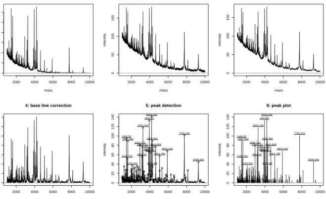
0.0e+00 5.0e+06 1.0e+07 1.5e+07 0.0e+00 5.0e+06 1.0e+07 1.5e+07 0.0e+00 5.0e+06 1.0e+07 1.5e+07 0.0e+00 5.0e+06 1.0e+07 1.5e+07 0.0e+00 5.0e+06 1.0e+07 1.5e+07 1 2 3 4 5 500 1000 1500 2000 M/Z Intensity Precursor M/Z 645.37,546.96,716.34,437.8 0.0e+00 5.0e+06 1.0e+07 1.5e+07 0.0e+00 5.0e+06 1.0e+07 1.5e+07 0.0e+00 5.0e+06 1.0e+07 1.5e+07 0.0e+00 5.0e+06 1.0e+07 1.5e+07 0.0e+00 5.0e+06 1.0e+07 1.5e+07 1 2 3 4 5 500 1000 1500 2000 M/Z Intensity Precursor M/Z 645.37,546.96,716.34,437.8 0 500000 1000000 1500000 2000000 500 1000 1500 M/Z Intensity Precursor M/Z 645.37 0 500000 1000000 1500000 2000000 114.0 114.4 114.7 115.0 115.3 115.6 115.9 116.2 116.5 116.8 117.1
Fig. 1: Plotting raw MS2data using functionality from theMSnbasepackage. On the left, the fullm/zrange
of an experiment containing 5 spectra is displayed. On the right, one spectrum of interest is illustrated,
highlighting the 4 iTRAQ reporter region. Both figures, have been created with the genericplotfunction,
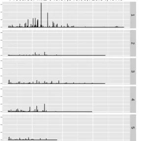
2000 4000 6000 8000 10000 0 5000 15000 25000 1: raw mass intensity 2000 4000 6000 8000 10000 0 50 100 150 2: variance stabilisation mass intensity 2000 4000 6000 8000 10000 0 50 100 150 3: smoothing mass intensity 2000 4000 6000 8000 10000 0 20 40 60 80 100 120 140
4: base line correction
mass intensity 2000 4000 6000 8000 10000 0 20 40 60 80 100 120 140 5: peak detection mass intensity ● ● ● ● ●●●●●● ● ●●● ● ●●● ● ● ● ● ● ●●● ● ● ● ● ● ● ● ● ● ● ● ● ● ●●●●● ● ●● ● ● ●● ● ● ● ● ● ● ● ● ● ● ● ● ● ● ● ●● ● ● ● ● ● ● ● ● ● ● ● ●● ● ● ● ● ● ● ● ● ●●● ●● ● ● ● ●● ● ● ● ● ● ● ● ●● ● ● ● ● ● ● ● ●● ● ● ● ● ● ● ●● ● ● ● ● ● ● ● ● ● ● ● ●●●●●● ● ●●● ●●● ● ● ●●● ● ●●● ● ● ● ● ● ● ● ● ● ● ● ● ●●● ● ● ●● ● ● ● ● 1466.05 1545.781 1617.063 2105.552 2932.711 3158.47 3192.143 3263.158 3883.32 3955.47 3972.747 4091.227 4210.261 4267.43 4282.581 4643.858 5064.799 5904.643 7765.216 9288.693 2000 4000 6000 8000 10000 0 20 40 60 80 100 120 140 6: peak plot mass intensity 1466.05 1545.781 1617.063 2105.552 2932.711 3158.47 3192.143 3263.158 3883.32 3955.47 3972.747 4091.227 4210.261 4267.43 4282.581 4643.858 5064.799 5904.643 7765.216 9288.693
Fig. 2: Label-free spectrum processing peak detection from the MALDIquant package. Figures represent
(1) raw data, (2) effect of variance stabilisation using square root transformation, (3) smoothing using a simple 5 point moving average, (4) base line correction, (5) noise reduction and peak detection and (6) final results.
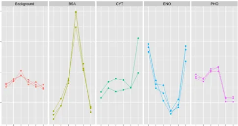
Background BSA CYT ENO PHO ● ● ● ● ● ● ● ● ● ● ● ● ● ● ● ● ● ● ● ● ● ● ● ● ● ● ● ● ● ● ● ● ● ● ● ● ● ● ● ● ● ● ● ● ● ● ● ● ● ● ● ● ● ● ● ● ● ● ● ● ● ● ● ● ● ● ● ● ● ● ● ● ● ● ● ● ● ● ● ● ● ● ● ● 0.1 0.2 0.3 0.4 126 127 128 129 130 131 126 127 128 129 130 131 126 127 128 129 130 131 126 127 128 129 130 131 126 127 128 129 130 131 Reporters Nor malised intensity
Fig. 3: Representation of peptide-level quantitation data. This plot has been generated using thePXD000001
TMT 6-plex data and converted to anMSnSetobject. Normalised background and spike (BSA, CYT, ENO
and PHO) reporter ion intensities for a subset of peptides have been plotted using theggplot2package [75].
MAVSKVYARSVYDSRGNPTVEVELTTEKGVFRSIVPSGASTGVHEALEMRDGDKSKWMGKGVLHAVKNVN 70
DVIAPAFVKANIDVKDQKAVDDFLISLDGTANKSKLGANAILGVSLAASRAAAAEKNVPLYKHLADLSKS 140
KTSPYVLPVPFLNVLNGGSHAGGALALQEFMIAPTGAKTFAEALRIGSEVYHNLKSLTKKRYGASAGNVG 210
DEGGVAPNIQTAEEALDLIVDAIKAAGHDGKIKIGLDCASSEFFKDGKYDLDFKNPNSDKSKWLTGPQLA 280
DLYHSLMKRYPIVSIEDPFAEDDWEAWSHFFKTAGIQIVADDLTVTNPKRIATAIEKKAADALLLKVNQI 350
GTLSESIKAAQDSFAAGWGVMVSHRSGETEDTFIADLVVGLRTGQIKTGAPARSERLAKLNQLLRIEEEL 420
GDNAVFAGENFHHGDKL 437
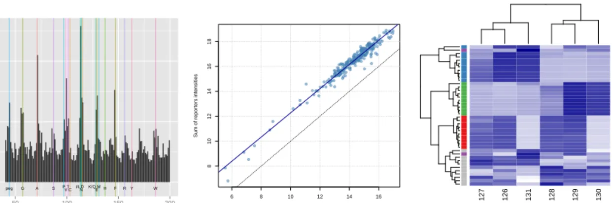
Fig. 4: Visualising observed peptides for the yeast enolase protein. Consecutive peptides are shaded in
peg G A S PVTCI/LNDK/Q MEH F RY W 0.00 0.01 0.02 50 100 150 200 m/z delta Density 6 8 10 12 14 16 8 10 12 14 16 18 Incompletedissociation S u m o f re p o rt e rs in te n s it ie s 127 126 131 128 129 130 Background Background Background Background Background Background Background Background Background CYT Background PHO PHO PHO PHO PHO PHO PHO PHO PHO PHO BSA BSA BSA BSA BSA BSA BSA BSA BSA BSA ENO ENO ENO ENO ENO ENO ENO ENO ENO CYT ENO
Fig. 5: Assessing the quality of the PXD000001 data set. On the left, the delta m/z plot illustrates the
relevance of the raw MS2 spectra for peptide identification. The middle figure compares fully dissociated
reporter signal against incompletely dissociated ions, indicating satisfactory reporter dissociation for the experiment. The last figure, a heatmap of a subset of peptides, highlights the expected lack of sample
grouping and tight peptides clustering. The first plot is produced by the plotMzDelta function from the
MSnbase package. The other figures used standard base R plotting functionality. The detailed code and
● ● ● ● ● ● ● ● ● ● ● ● ● ● ●● ● ● ● ● ● ● ● ● ● ● ● ● ● ● ●● ● ● ● ● ● ● ● ● ● ● ● ● ● ● ● ● ● ● ● ● ● ● ● ● ● ● ● ● ● ● Spectra MA plot
log10 average intensity
ratio channel 127 vs 129 4 5 6 7 0.2 0.5 1.0 2.0 5.0 ● ● ● ● BSA ENO CYT PHO ● ● ● ● −0.6 −0.4 −0.2 0.0 0.2 0.4 0.6 0 2 4 6 8 10
Protein volcano plot
log10 fold−change
− lo g10 p − v a lu e ● ● ● ●
Fig. 6: On the left, the MA plot for thePXD000001127 vs. 129 reporter ions, showing the 95% confidence
intervals of the background peptides (red), spikes (blue) and all (green) peptide noise models. The respective
peptides are colour-coded according to the proteins. The volcano plot on the right illustrates protein
significance (−log10 p-value) as a function of the log10 fold-change. The vertical coloured dashed indicate
the expected log10 ratios. The black dotted horizontal and vertical lines represent a p-value of 0.01 and
ups25a (m25a×1) asMSnSet ms25a (m25a×1) topN ups25b (m25b×1) asMSnSet ms25b (m25b×1)
topN combine (m25ms25×3) filterNA
ups25c (m25c×1) asMSnSet ms25c (m25c×1) topN ups50a (m50a×1) asMSnSet ms50a (m50a×1) topN ups50b (m50b×1) asMSnSet ms50b (m50b×1) topN combine ms50 (m50×3) filterNA ups50c (m50c×1) asMSnSet ms50c (m50c×1) topN combine final (mf inal×6)
Fig. 7: The synapter to MSnbase pipeline, illustrating how to combine and process data objects in an
design specific work flow. Data objects are represented by grey boxes, while functions, that manipulate and transform the objects are shown in white boxes. The respective dimensions of the objects (number of