System Simulation of RF Front-End Transceiver for
Frequency Modulated Continuous Wave Radar
ABSTRACT
Frequency modulated continuous wave (FMCW) radar is a solution for range and velocity measurement of a target. This paper introduces a simulation methodology for a RF front-end transceiver of a FMCW radar system including the target model. The proposed system model can incorporate realistic design conditions such as voltage controlled oscillator phase noise. The methodology has been applied to a 2.45 GHz FMCW radar with a single antenna for transmitting and receiving waves using Advanced Design System (ADS) simulation package from Agilent. Various values of target range and velocity are employed in the simulated model to verify the operation of the FMCW radar system. The proposed simulation model has been proven to be a useful tool in the design of FMCW radar systems. The system model is used to conclude some general guidelines to help the system designer.
Keywords
FMCW radar, Velocity, Doppler, Circulator, LNA.
1.
INTRODUCTION
Radar systems are being used in many applications nowadays. There are different types of radar systems; one of the well-known radar systems is FMCW. FMCW radar systems have applications in various fields ranging from civil to military applications. FMCW radars can be used for imaging purposes ([1]-[4]); automotive FMCW radar can be used to record velocity violations on roads [5,6]. They can be also used as driver assistance systems to improve driving conditions and avoid collisions [7]. They can be also employed for ship navigation and identification as proposed by Duarte et. al. [8]. FMCW radars can be used for target detection under the ground clutter environment [9]. Some authors presented FMCW radars for geosciences to measure wind speed and direction [10] or to perform surface analysis to planets [11]. On the other hand, it is frequently used for military purposes to monitor and to guide airplanes and missiles [12].
In the frequency-modulation method, the transmitter radiates radio-frequency waves. The frequency of these RF waves is continually increasing and decreasing from a fixed reference frequency. At any instant, the frequency of the returned (reflected) signal differs from the frequency of the radiated one. The amount of the difference in the frequency is determined by the time it took the signal to travel the distance from the transmitter to the target [13].
In the system design of the RF front-end transceiver, a designer uses Friis equation and IP3 cascaded system equation for noise and nonlinearity estimate. The designer employs these equations to distribute the system specifications to the individual receiver blocks. Aleksandar et. al. [14] introduced a procedure for optimal allocation of the performance parameters to the individual RF front-end circuit blocks based on these two equations. However, there should be a simulating methodology to gain exactness of the system design as these two equations have their limitations. For the first time, to the best of our knowledge, a system level simulation methodology is proposed and thoroughly explained. The model of the target is included; the VCO phase noise has been also modeled in the simulation. Other effects, although not included, can be easily incorporated in the simulation. For example, one can model the attenuation and noise carried by the channel between the antenna and the target model.
The operation principle of the FMCW radar is discussed in section 2. Section 3 presents the generation of the FM chirp waveform and the frequency deviation relationship to the target range. Section 4 describes the development of the target model while section 5 explains the whole system model supported with simulation results. Some general design guidelines are withdrawn for the system designer. The article is finally concluded in section 6.
2.
PRINCIPLE of FMCW RADAR
The carrier signal of the radar is frequency-modulated in linear ramps. The antenna of the radar transmits and receives simultaneously with a frequency deviation (ΔF) for both the transmitted and received signals, as shown in figure 1. The frequency difference (Fr) is proportional to the time difference
between the transmitted and received signals, which in turn is proportional to the distance between the transmitter and the reflecting-object (target).
In a regular FMCW radar, the frequency sweep over ΔF Hz in T second at the carrier frequency is transmitted. The receiver mixes the transmitted signal with the delayed received signal; the output of the mixer constitutes the frequency difference and sum components. The mixer is followed by a low pass filter in order to pass the frequency difference component only. This is referred to a beat note whose frequency Fr is
proportional to the range R of a stationary target or a target whose velocity produces a Doppler shift larger than ±1/2T Hz [15].
Ahmed M. Eid
Department of Electrical Engineering, Faculty of Engineering and Islamic
Architecture,
Umm Al Qura University, Makkah, Saudi Arabia
Ahmed M. Nahhas
Department of Electrical Engineering, Faculty of Engineering and Islamic
Architecture,
Assume that the transmitter frequency increases linearly with time and that there is a reflecting object at a distance r = ro, A
frequency modulated carrier signal can be written as:
Fig 1: Range determination of stationary target
) t ( cos A
us s s (1)
t T F f ) t (
fs o
for 0tT (2)
so 2 o t 0 so s s t T F 2 1 t f 2 dt ) t ( f 2 ) t (
(3)where Asis the signal amplitude, fo the carrier frequency,
φso the initial phase, and fs(t) a time varying frequency. An
echo signal will return after the transit time τ. The phase of the received signal can be expressed as:
So 2 o
s
E (t )
T F 2 1 ) t ( f 2 ) t ( ) t (
(4)
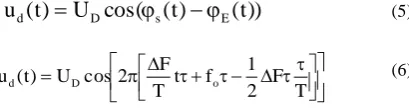
If the echo signal is heterodyned with a portion of the transmitter signal in a nonlinear element such as a diode, a beat note will be produced. The beat note component can be written as:
))
t
(
)
t
(
cos(
U
)
t
(
u
d
D
s
E (5) T F 2 1 f t T F 2 cos U ) t (
ud D o (6)
where UD is the amplitude of the beat note signal. If there is
no Doppler frequency shift (non moving target), the beat note (difference frequency) is a measure of the target's range.
o o
c
r
2
(7) F
Fr (8)
where co is the velocity of light. The resolution limit of the
measured beat note frequency is determined by the time span T:
T
1
F
r
(9)If we have two targets with ranges r1 and r2, their beat note
frequencies can be estimated as, using equations (7) and (8):
o 1 1 r
c
r
2
T
F
F
(10)o 2 2 r
c
r
2
T
F
F
(11)The resolution limit of the beat note frequency can be determined by: o 1 o 2 1 r 2 r r c r 2 c r 2 T F F F
F (12)
Equating equations (9) and (12), the resolution limit of the measured range can be calculated as:
F
2
c
r
r
r
o 1 2
(13)If a target is moving with a linear velocity vr relative to the
radar, a Doppler shift Fd is introduced which shifts the
received signal in frequency. Figure 2 illustrates the received frequency compared to that of a stationary target.
[image:2.595.60.237.131.231.2]Distance (range) r of an object moving with a relative velocity(vr) at time t can be determined as:
Fig 2: Calculation of the velocity of a Moving target using the Doppler frequency shift
t
v
r
r
o
r
(14)Round-trip travel time is written as:
o r o o
c
t
v
2
c
r
2
)
t
(
(15) [image:2.595.73.278.574.628.2]
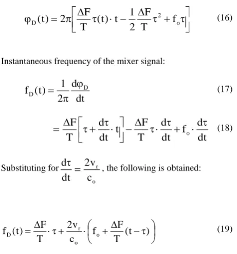
2 oD
f
T
F
2
1
t
)
t
(
T
F
2
)
t
(
(16)
Instantaneous frequency of the mixer signal:
dt
d
2
1
)
t
(
f
DD
(17)dt
d
f
dt
d
T
F
t
dt
d
T
F
o
(18)Substituting for
o r
c
v
2
dt
d
, the following is obtained:
(t )
T F f c
v 2 T
F ) t (
f o
o r
D (19)
The first term is equal to Fr defined by equation (8) where is
approximately constant during measurement. Since the maximum time shift (t-) is equal to T and F is typically much less than fo, the second term is approximately equal to
Doppler frequency Fd; where:
o r o d
c
v
2
f
F
(20)So if there is a moving target, a Doppler frequency shift will be superimposed on the FM range beat note and an erroneous range measurement results. The Doppler frequency shift causes the frequency-time plot of the echo signal to be shifted up or down, as shown in Figure 2. On one portion of the frequency-modulation cycle, the beat frequency is increased by the Doppler shift, while on the other portion, it is decreased. If for example, the target is approaching the radar, the beat frequency produced during the frequency-increasing portion of the FM cycle will be the difference between the beat frequency due to the range Fr and the Doppler frequency
shift Fd:
d r 1
D
F
F
f
(21)Similarly, on the decreasing portion, the beat frequency is the sum of the beat frequency due to the range Fr and the Doppler
frequency shift (Fd):
f
D2
F
r
F
d (22)fD1 and fD2 are measured from which the range (ro) and
velocity (vr) can be calculated simultaneously.
3. LINEAR FM CHIRP WAVEFORM
GENERATION
The VCO is used in the system level simulations in order to produce the required transmitter signal. The VCO is modulated with a triangular source to produce a FMCW, as shown in figure 3. This chirp waveform, shown in figure 4, is used in high-resolution radars for small-target detection and target recognition. The radio frequency is increased at a constant rate from the carrier frequency fo to f = fo +Δf where
Δf is the sweep bandwidth, as shown in figure 2, where T is the modulation period. This type of modulated waveform gets its bandwidth from the modulation and not the pulse width as for a waveform modulated with rectangular pulses whose spectrum has high frequencies. The chirp waveform bandwidth is given by the sweep bandwidth (Δf). With this waveform it is possible to have wide bandwidths, giving good range resolution as indicated by equation (13), and wide pulse widths, giving a higher average radiated power and thus a higher probability of detection. For example, a sweep bandwidth Δf = 500 MHz gives a range resolution of
f
2
c
R
o
= 68
10
x
500
x
2
10
x
3
=0.6 m (23)
[image:3.595.53.284.68.316.2]The linear modulation is continued for a period, (T), at least several times as long as the roundtrip transit time for the most distant target.
Fig 3: ADS schematics for linear modulations
0.5 1.0 1.5 2.0 2.5
0.0 3.0
2.42 2.44 2.46 2.48
2.40 2.50
time, usec
re
al
(O
sc
[0
])
Fig 4: VCO time domain signal
0.2 0.4 0.6 0.8 1.0 1.2 1.4 1.6 1.8 2.0 2.2 2.4 2.6 2.8
0.0 3.0
-0.2 0.0 0.2
-0.4 0.4
time, usec
r
e
a
l
(
o
sc[
1
]
)
Time (micro-Seconds)
Real
(
OSI
[1]
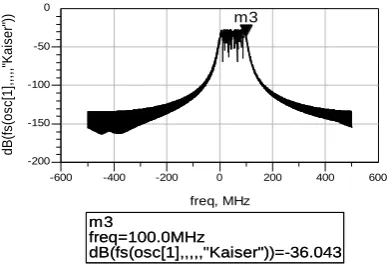
Fig 5: VCO Spectrum
[image:4.595.62.273.317.458.2]In the VCO spectrum, shown in figure 5, the X-axis is not the absolute frequency, but the offset from the nominal analysis frequency, set at the carrier frequency. The actual spectrum of the VCO is shown in figure 6 which is used in the transient analysis. In both figures, it is obvious that the bandwidth is equal to the sweep bandwidth f = 100 MHz.
Fig 6: VCO Spectrum using transient simulation
4. DOPPLER TARGET MODEL
The frequency of a signal reflected by a moving target is modeled. As explained previously, the moving target introduces Doppler frequency shift compared to a stationary target. If the transmitter’s signal at an arbitrary frequency is given by:
)
t
cos(
E
E
t
o
(24)The echo signal from a moving target will be:
KE
cos
t
E
r o d (25)where
K
: Constant determined from the radar equation.,o
E
: Amplitude of the transmitter signal.
: Angular frequency from transmitter, rad/s.
: Constant phase shift.The positive sign, in equation (25), indicates approaching target while the minus sign indicates diverging target. Equation (25) can be rewritten as:
t
t
cos
KE
E
r
o
d (26)Using the trigonometric identity
B
sin
A
sin
B
cos
A
cos
)
B
A
cos(
,equation (25) can be written as:
cos
t
cos
t
sin
t
sin
t
KE
E
r
o
d
d (27)The phase shift
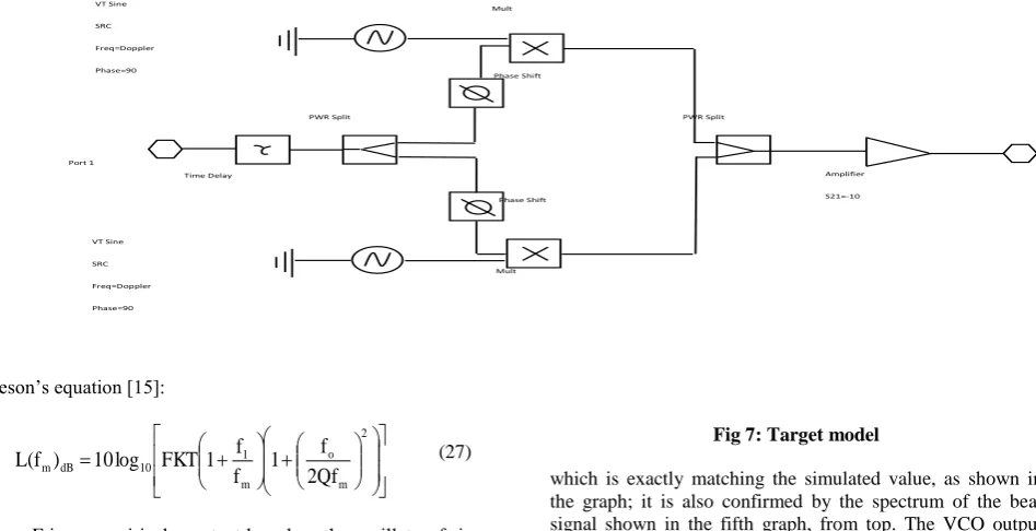
results from the transit time due to ranging.Equation (26) can be implemented in the target model, shown in figure 7, using HP-Advanced Design System (ADS). It can be also implemented in other SPICE-like circuit simulators. This model receives an incident signal and generates the corresponding reflected signal from a generally moving target. The incident is first delayed by the transit time calculated by equation 7. The signal is then divided equally by a power splitter. One of the outputs of the power divider passes through a phase-shifter with 900 phase shift while the other one goes unchanged. As a result, the outputs of the phase-shifters are quadratic to form the cos(t+) and sin(t+) terms. These signals are then multiplied by the corresponding quadratic signals cos(dt) and sin(dt),respectively. The outputs of the multipliers are added up using a power combiner. The amplitude of the reflected signal is then controlled by an amplifier block to model the radar, environment, and target properties.
5. SYSTEM MODEL AND SIMULATION
RESULTS
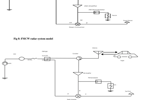
Figure 8 demonstrates the block diagram of a FMCW radar system model as implemented using ADS. It consists mainly of a transmitter and a receiver as well as a target model. The target model was described in the previous section. The transmitter path starts by a linear FM chirp waveform generator. The output of the generator goes into a power splitter in order to feed the mixer of the receiving path. The other output of the splitter is applied to a circulator from which it is directed to the antenna. The transmitted signal, by the antenna, hits the target, represented by an automobile symbol.
The reflected signal is modeled into the target, and then returned back to the antenna. The received signal, by the antenna, goes to the circulator from which it is directed to the LNA followed by a mixer. The LNA output signal is mixed with a portion of the transmitted signal to generate the beat note signal. The low frequency beat note signal is automatically filtered out in the mixer-IF block. The beat signal frequency is then analyzed to calculate the distance and velocity of the target.
Phase noise may be added to the VCO, via the phase noise
m3
freq=100.0MHz
dB(fs(osc[1],,,,,"Kaiser"))=-36.043 m3
freq=100.0MHz
dB(fs(osc[1],,,,,"Kaiser"))=-36.043
-400 -200 0 200 400
-600 600
-150 -100 -50
-200 0
freq, MHz
d
B(f
s
(o
s
c
[1
],
,,
,,
"Ka
is
e
r"
)) m3
m1
freq=2.405GHz dB(fs(osc))=-26.983
m2
freq=2.496GHz dB(fs(osc))=-28.129 m1
freq=2.405GHz dB(fs(osc))=-26.983
m2
freq=2.496GHz dB(fs(osc))=-28.129 2.1 2.2 2.3 2.4 2.5 2.6 2.7 2.8 2.9
2.0 3.0
-140 -120 -100 -80 -60 -40
-160 -20
freq, GHz
d
B
(f
s(
o
sc)
)
Leeson’s equation [15]:
2
m o m
1 10
dB m
Qf 2
f 1 f
f 1 FKT log 10 ) f (
L (27)
where F is an empirical constant based on the oscillator, f1 is
another constant, Q is the quality factor, K is Baltzmann’s constant, T is the temperature in Kelvin, and fm is the offset
frequency from the carrierfrequency fo.
5.1.1 Stationary target
In the case of a stationary target, velocity is set at 0 Km/s while range is arbitrary chosen as 40 m. The sweep frequency f is equal to 100 MHz with a sweep period T = 0.5 s. It is worthy to mention that the sweep period is typically in the range of hundreds of microseconds. The value here is short, without loss of general, in order to increase the sweep frequency; and consequently reduce the simulation time as it is governed by the lowest frequency in the system. The transit time estimated in the target model is equal to:
Figure 10 demonstrates the simulation results using our system model with the stationary target. On the top of the figure, baseband signals represent both the modulating signal of the transmitter and the demodulated signal of the receiver after the LNA. The two signals experience a time shift equal
to the transit time. The beat signal and its frequency are displayed in the third and second graphs from top, respectively. The maximum value of the beat frequency( Fr )
[image:5.595.64.538.132.375.2]can be estimated as, using equation (8):
Fig 7: Target model
which is exactly matching the simulated value, as shown in the graph; it is also confirmed by the spectrum of the beat signal shown in the fifth graph, from top. The VCO output signal and its spectrum are shown in the Fourth and sixth graphs. The bandwidth is almost equal to the sweep frequency 100 MHz.
The simulation results for the stationary target assure the sanity of the model. They also demonstrate how the received signal can be processed in order to ultimately measure the range of the target.
5.1.2 Moving target
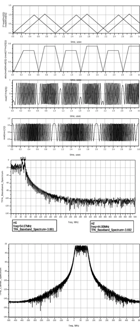
A moving target is considered with a velocity of 300 Km/s and a range of 37.5 m. The velocity is scaled up to a virtual velocity for any craft in order to be compatible with the short sweep period. Once again, the system is still general and these numbers are scaled in order to shorten out the simulation time without loss of generality. The same sweep frequency f of 100 MHz with a sweep period 0.5 s is employed.
ns
267
10
x
3
/
40
*
2
8
MHz
53
10
x
267
.
0
x
10
x
5
.
0
10
x
100
F
6 66
r
Time Delay Port 1
PWR Split PWR Split
Phase Shift
Phase Shift
Mult Mult
Amplifier S21=-10 VT Sine
SRC Freq=Doppler Phase=90
Fig 8: FMCW radar system model
Fig 9: FMCW radar system model with phase noise added to VCO
The new transit time can be evaluated to 250 ns. The simulation results are shown in figure 11. The modulating and demodulated signals are shown on the top of the figure. The demodulated signal is shifted up indicating Doppler frequency shift. The Doppler frequency shift and range frequency can be calculated, using equations (20) and (8), respectively, as:
VCO Freq=2.4 GHz
Vt pulse
50 Ohm
PWR Split
S21=0.707 S31=0.707
Circulator
Antenna
LNA Amplifier
Target
Down Converter IF RF LO
Test Point FM Demodulator
Term 50 Ohm Vt pulse
Circulator
Antenna
LNA Amplifier
Target
Down Converter IF RF LO
Test Point FM Demodulator
Term 50 Ohm Phase Noise
PWR Split S21=0.707 S31=0.707 50 Ohm
VCO Freq=2.4 GHz
MHz
50
10
x
25
.
0
x
10
x
5
.
0
10
x
100
F
6 66
r
MHz
8
.
4
10
x
3
10
x
300
x
2
x
10
x
4
.
2
F
83 9
[image:6.595.55.531.137.471.2]Fig 10: Stationary target with range 40 m
The second graph from top demonstrates the frequency of the beat signal with two distinct levels at the difference fD1 = 45.2
MHz and sum fD2 = 54.8 MHz. These results are in good
conformity with the theoretical analysis. The spectrum of the beat signal, in the fifth graph, obviously has two peaks at almost same frequencies. In typical radars, these two frequencies can be used to estimate Fr and Fd from which
velocity and range can be calculated. The VCO output signal and its spectrum are shown in the fourth and sixth graphs. The bandwidth is almost equal to the sweep frequency 100 MHz.
Fig 11: Moving target with a virtual velocity of 300 Km/s and a range of 37.5 m
5.2 Practical Considerations
Some practical considerations can be inferred from simulations of our system model. These considerations impact the system level performance and should be taken into account during the distribution of the block level specifications. Some general guidelines for the system level designer can be used. Typical numbers of block level parameters differ from system to another. They depend on the whole system design, which is based on the technology and required specifications of the system.
0.2 0.4 0.6 0.8 1.0 1.2 1.4 1.6 1.8 2.0 2.2 2.4 2.6 2.8
0.0 3.0
0
-1 1
time, usec
real(T
PA[
0]
)
0.2 0.4 0.6 0.8 1.0 1.2 1.4 1.6 1.8 2.0 2.2 2.4 2.6 2.8
0.0 3.0
0.0
-0.5 0.5
time, usec
real(os
c
[1]
)
0.2 0.4 0.6 0.8 1.0 1.2 1.4 1.6 1.8 2.0 2.2 2.4 2.6 2.8
0.0 3.0
0.0 0.5
-0.5 1.0
time, usec
real(M
od[
0]
)
2*
real(f
m
[0]
)
m1 freq=53.00MHz
TPA_Baseband_Spectrum=-470.1m m1
freq=53.00MHz
TPA_Baseband_Spectrum=-470.1m
20 40 60 80100120140160180200220240260280300320340360380400420440460480
0 500
-140 -120 -100 -80 -60 -40 -20
-160 0
f req, MHz
T
PA_Bas
eband_Sp
ec
trum
m1
-450 -400 -350 -300 -250 -200 -150 -100 -50 0 50 100 150 200 250 300 350 400 450
-500 500
-120 -100 -80 -60 -40
-140 -20
f req, MHz
T
PB_C
arrier_Spec
trum
0.2 0.4 0.6 0.8 1.0 1.2 1.4 1.6 1.8 2.0 2.2 2.4 2.6 2.8
0.0 3.0
0.2 0.4
0.0 0.6
time, usec
beat
_f
requenc
y
0.2 0.4 0.6 0.8 1.0 1.2 1.4 1.6 1.8 2.0 2.2 2.4 2.6 2.8
0.0 3.0
0
-1 1
time, usec
real(T
PA[
0]
)
0.2 0.4 0.6 0.8 1.0 1.2 1.4 1.6 1.8 2.0 2.2 2.4 2.6 2.8
0.0 3.0
-0.5 0.0 0.5
-1.0 1.0
time, usec
real(os
c
[1]
)
0.2 0.4 0.6 0.8 1.0 1.2 1.4 1.6 1.8 2.0 2.2 2.4 2.6 2.8
0.0 3.0
0.5 1.0
0.0 1.5
time, usec
real(M
od[
0]
)
2*
real(f
m
[0]
)
m1 freq=54.67MHz
TPA_Baseband_Spectrum=-3.861
m2 freq=44.00MHz
TPA_Baseband_Spectrum=-3.692 m1
freq=54.67MHz
TPA_Baseband_Spectrum=-3.861
m2 freq=44.00MHz
TPA_Baseband_Spectrum=-3.692
20 40 60 80100120140160180 200220240260280300320340360380400420440460480
0 500
-120 -100 -80 -60 -40 -20
-140 0
f req, MHz
T
PA_Bas
eband_Sp
ec
trum
m1 m2
-450 -400 -350 -300 -250 -200 -150 -100 -50 0 50 100 150 200 250 300 350 400 450
-500 500
-160 -140 -120 -100 -80 -60 -40
-180 -20
f req, MHz
T
PB_C
arrier_Spec
trum
0.2 0.4 0.6 0.8 1.0 1.2 1.4 1.6 1.8 2.0 2.2 2.4 2.6 2.8
0.0 3.0
0.2 0.4
0.0 0.6
time, usec
abs
(real(M
od[
0]
)-(real(2*
fm
[0]
[image:7.595.324.549.76.599.2]5.2.1 Effect of rejection parameters of the mixer
System level simulations explain that rejection parameters of the mixer LO_rej1 and LO_rej2 should be large. LO_rej1 and LO_rej2 parameters are the local oscillator signal to input port rejection and output port rejection in dB, respectively. The reason is that low values of these rejection parameters result in higher values of DC component in the output spectrum. Such DC component can saturate subsequent block. On the other hand, the RF signal to output port rejection RF_rej has no effect. This is can be justified by the low power of the reflected signal.
5.2.2 Effect of isolation parameters of the
circulator
Circulator isolation from the transmitter port to the receiver port should be high. If the isolation is not large enough, some transmitted power can leak into the receiving path resulting in saturation of the LNA and subsequent blocks.
5.2.3 Effect of gain and noise-factor of LNA
The gain of the low-noise-amplifier LNA, indicated by S21,
should be large while its noise factor (NF) should be low. These are basic requirements for the LNA to get a low value for the overall NF of the receiving path. Specifically, a high gain for the LNA before the mixer is important to make it easy to resolve the weaker target echo.
The noise factor (NF) of the LNA has been swept from 3 dB to 21 with S21 fixed at 5 dB. Simulations demonstrated an
evident change in the output for different values of NF.
6. CONCLUSIONS
A full RF front-end transceiver of a FMCW radar system model has been proposed and simulated. The simulation methodology has been implemented in ADS; however it is applicable to other SPICE-like circuit simulators. The model includes typical receiving and transmitting paths along with target model. The development of the target model has been provided. VCO phase noise has been also incorporated into the system model. The system model is flexible to adapt other realistic effects such as channel model. The channel model can be inserted between the antenna and the target model to accommodate for the attenuation and noise of the channel. The system has been simulated for stationary as well as moving targets. The simulation results showed good agreement with theoretical ones. Finally, some practical considerations were concluded for RF front-end system designers.
7. REFERENCES
[1] J. Schellenberg, R. Chedester, and McCoy, J. 2007, Multi-Channel Receiver for an E-band FMCW Imaging Radar, IEEE/MTT-S International Microwave Symposium, 1359-1362.
[2] Zhang, Y. Yin, Z. Chen, W. and Wang, D. 2007, Two-dimensional radar imaging based on instant range profile, 1st Asian and Pacific Conference on Synthetic Aperture Radar, APSAR 2007, 236-239.
[3] Asensio-Lopez, Blanco-del-Campo, A. Gismero-Menoyo, J. Ramirez-Moran, Torregrosa-Penalva, D. Dorta-Naranjo, B. and Carmona-Duarte, C. 2004, High range-resolution radar scheme for imaging with tunable distance limits, Electronics Letters , Vol. 40, 17, 1085-1086.
[4] Cooper, K. Dengler, R. Chattopadhyay, G. Schlecht, Gill, E. Skalare, A. Mehdi, I. and Siegel, P. 2008, A High-Resolution Imaging Radar at 580 GHz, IEEE Microwave and Wireless Components Letters, Vol. 18, 1, 64-66.
[5] Winkler, V. 2007, Range Doppler detection for automotive FMCW radars, European Microwave Conference, 1445-1448, 9-12.
[6] Ali, F., Vossiek, M. 2010, Detection of weak moving targets based on 2-D range-Doppler FMCW radar Fourier processing, German Microwave Conference, 214,217, 15-17.
[7] Steinhauer, M. Ruo, H. Irion, H. and Menzel, W. 2008, Millimeter-Wave-Radar Sensor Based on a Transceiver Array for Automotive Applications, IEEE Transactions on Microwave Theory and Techniques, Vol. 56, 2, 261-269.
[8] Park, S. and Kim, Y. 2011, Designing of a low resolution FMCW radar for small target detection underground clutter, Synthetic Aperture Radar (APSAR), 3rd International Asia-Pacific Conference 1,1, 26-30.
[9] Duarte, C., Naranjo, P., Dorta, A., Lopez, A. and del Campo, A. 2007, CWLFM Radar for Ship Detection and Identification, IEEE Aerospace and Electronic Systems Magazine, Vol. 22, 2, 22-26.
[10]Nekrasov, A. and Hoogeboom, P. 2005, A Ka-band backscatter model function and an algorithm for measurement of the wind vector over the sea surface, IEEE Geoscience and Remote Sensing Letters, Vol. 2,1, 23-27.
[11]Leuschen, C., Kanagaratnam, Yoshikawa, K., Arcone, S. and Gogineni, P. 2002, Field experiments of a surface-penetrating radar for Mars, IEEE International Geoscience and Remote Sensing Symposium, IGARSS '02, Vol. 6, 3579-3581, 24-28.
[12] Jahagirdar, R. 2012, A high dynamic range miniature DDS-based FMCW radar, Radar Conference (RADAR), IEEE, 0870,0873, 7-11.
[13]Skolink, M. 1980, Introduction to Radar Systems, McGraw Hill, New York, NY.
[14]Aleksandar, T., Wouter, S., and John L. 2004, Optimal Distribution of the Front-End System Specifications to the RF Front-End Circuit Blocks, IEEE Conference Proceedings ISCAS, Vol. I, 889-892.