The effects of exports, aid and remittances on output: The case of Kiribati

Munich Personal RePEc Archive

The effects of exports, aid and

remittances on output: The case of

Kiribati

Rao, B. Bhaskara and Takirua, Toani

University of the South Pacific

1 July 2006

The Effects of Exports, Aid and Remittances on Output: The Case of Kiribati

B. Bhaskara Rao and Toani B Takirua1

University of the South Pacific Suva (Fiji Islands)

Abstract

Country specific time series models of the determinants of output for the small developing

island countries in the Pacific region are relatively few. This paper explores the applicability of

the framework underlying Solow (1956) to analyze the determinants output in Kiribati for the

period 1970-2005. It is found that technical progress in Kiribati has been negative virtually

offsetting the positive effects of factor accumulation. Aid and remittances have negative effects

and exports have only a small positive effect in the short run.

Keywords: Kiribati, Growth, Aid, Exports and Remittances

1 The authors are respectively Professor of Economics (contact author) and graduate student. Email for the contact

1. Introduction

The purpose of this paper is to explore the use of the Solow (1956) model and its extended

versions. This is a relatively unexplored area for the Pacific Island countries (PICs) except for

Fiji by some University of the South Pacific (USP) economists like Rao, Singh and Fozia (2006)

and Rao and Rao (2006). In doing so, we analyze the significance of the exports, remittances

and aid, besides the two basic conditioning variables viz., capital (K) and labour (L), for the

determination of output in Kiribati.2 Our approach differs from many ad hoc applications where

the growth rate of output is simply regressed on any variable (e.g., defense expenditure) or a set

of variables without incorporating the conditioning variables into the specification. At the least

this amounts to gross misspecification and the effects of the selected variables may be

overestimated. Such ad hoc studies are too many to cite. We shall later use one or two examples

to illustrate some weaknesses of such ad hoc specifications.

The aforesaid USP methodology of Rao et al which is used in this paper is similar to the

Mankiew, Romer and Weil (1992), MRW hereafter, extension to the Solow model in which the

basic neoclassical Cobb-Douglas production function is augmenting with shift variables like

human capital. MRW found that the Solow residual, which actually is a measure of our ignorance of the determinants of growth rate, could be considerably reduced without the need

for changing the basic simplifying assumptions of the Solow model.Acemoglu (2004) considers

the work of MRW as an attempt to revive the usefulness of the basic Solow growth model; see

also Rao and Singh and Nisha (2006) and Asteriou and Price (2004). Our attempt in this paper

with time series data modifies the MRW extension to the Solow model with cross section data.

At the outset, it may be stated that although it is desirable to use a few alternative methods of

estimating cointegrating equations, only the general to specific approach (GETS) of Hendry and

2 Kiribati consists of 33 atoll islands with a total land area of 811 square kilometers, lying astride the equator

situated in a 3.6 million square kilometers of its Exclusive Economic Zone. Its population in 2005 was about

the systems based Johansen Maximum Likelihood techniques (JMLVECM) yielded meaningful

results for our data. Furthermore, we have used the instrumental variable approach in the single

equation GETS approach to minimize any endogenous variable bias. Needless to say these two

techniques are second to one.Nevertheless, given the exploratory nature of our attempt,

whatever policy implications are derived from our empirical estimates need further

investigations. Therefore, our findings should be interpreted cautiously.

This paper is organized as follows. Unit root test results are in Section 2. Section 3 contains the

specification and cointegration issues. Various empirical results with the basic and extended

Solow model are in Sections 4 and 5 respectively. Section 5 also contains results with ad hoc

specifications. Section 6 concludes.

2. Unit Roots

The purpose of unit root tests is to test for the stationarity of a time series. Stationary series are

said to be integrated of order zero I(0). There are alternative unit root test procedures, each

claiming that it has more power against the null of unit root in a variable. Therefore, we shall

use some popular alternative tests to test for unit roots in the logs of our variables viz., output

per worker (ln )y , capital per worker (ln )k , export ratio which is export divided by output

(lnEX), aid as ratio to output (lnAID)and remittance ratio which is measured as real

remittances divided by employment (lnREM). In doing so, the following tests are used viz.,

the augmented Dickey Fuller (ADF), the ADF with generalized least squares (ADFGLS) of

Pantula (xxxx) which is more powerful than OLS based ADF, the Phillips-Perron

non-parametric test (PP), KPSS and the Elliot-Rothenberg-Stock test (ERS).3 These tests did not

yield uniform results, but it is generally believed that ADFGLS and ERS are more powerful and

these two tests indicate that all our variables are unit root variables. To conserve space we only

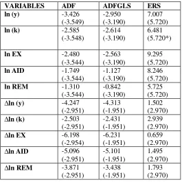
report ADF, ADFGLS and ERS test results in Table 1.

Our unit root test results are as follows. The null hypothesis of unit root is rejected in first

difference in all of the variables except for ∆lnk under the ADF, PP and KPSS where we did

not report the results based on PP and KPSS. However, the two powerful tests viz., GLSADF

and ERS show that ∆lnk is a stationary variable. Therefore, we may conclude that we can proceed and utilize cointegration techniques to estimate the long run relationships between

output and the other variables shown in Table 1.

Table 1. Unit Root Tests Results

VARIABLES ADF ADFGLS ERS ln (y) -3.426

(-3.549)

-2.950 (-3.190)

7.007 (5.720)

ln (k) -2.585 (-3.548)

-2.614 (-3.190)

6.481 (5.720*)

ln EX -2.480 (-3.544)

-2.563 (-3.190)

9.295 (5.720)

ln AID -1.749 (-3.544)

-1.127 (-3.190)

8.246 (5.720)

ln REM -1.310 (-3.544)

-0.842 (-3.190)

5.725 (5.720) ∆ln (y) -4.247

(-2.951)

-4.313 (-1.951)

1.502 (2.970) ∆ln (k) -2.503

(-2.951)

-2.431 (-1.951)

2.939 (2.970) ∆ln EX -6.198

(-2.954)

-6.231 (-1.951)

0.659 (2.970) ∆ln AID -5.096

(-2.951)

-5.101 (-1.951)

1.495 (2.970) ∆ln REM -3.871

(-2.951)

-3.438 (-1.951)

1.793 (2.970)

Notes: Figures in brackets are the 5% level critical values. While in tests for the levels of the variables intercept and trend are included, trend is not present in the tests for their first

differences. The null hypothesis in ADF and GLSADF is that the variable contains a unit root. In ERS the null is that the variable is stationary.

3.1 Cointegration

Where variables are in their levels I(1) and therefore I(0) in their first differences, means that

such variables with a long run equilibrium relationship cannot drift very far apart because

economic forces will act to correct any disequilibrium. In other words errors have a tendency to

become small and will become I(0). Therefore, we now employ some popular techniques of

cointegration to estimate a baseline long run output equation and then estimate the short run

Engle-Granger, Fully Modified Ordinary Least Squares (FMOLS) and JMLVECM are used. However,

only GETS and JMLVECM have given plausible results. These techniques will be used in the

rest of this paper to examine whether or not variables like aid ratio, export ratio and remittance

ratio have any effects besides the basic inputs of labour and capital. To conserve space we shall

not report results with FMOLS and Engle-Granger methods.

3.2 The Model

In this empirical work, the basic Solow (1956) model and its extension by MRW is used.

Therefore, some assumptions should be noted. Firstly, unlike in the cross section work with the

Solow model where the steady state growth equation is estimated, in the time series what is

estimated is the basic Cobb-Douglas production function and not the growth rate of output.

Because of the transformations necessary to use time series methods (to overcome unit root

problem), the dependent variable is the rate of growth of output. This does not mean that the

estimated equation is the steady state growth equation and many applied workers mistake this to

be so. This is not correct. What is estimated in time series models is the steady state production

function. To derive steady state growth equation, this production function should be combined

with other equations in the Solow (1956) growth model. Second, we also assume that there are

constant returns and unlike in Solow (1956) technology is Hicks neutral. Third, additional

variables, such as the export ratio etc., are introduced into the model as shift variables into the

production function. We feel that this is adequate for our purpose although these additional

variables can be introduced into the production function in other different ways. Essentially we

follow Rao and Rao (2006) and our basic production function with constant returns and Hicks

neutral technical progress is:

Y

= A

K

L

= A

e

K

L

where A0 represents the initial stock of knowledge, t is time, K is capital and L is labour. An

important assumption for illustrative purpose is that the stock of knowledge not only changes

ratio of exports or the ratio of aid to output etc. Now Z may have a permanent and/or a

temporary effect on output. To distinguish between the temporary and permanent effects of Z,

these following procedures are used. The first procedure is to include Z in the cointegrating

equation with capital and labour inputs. The latter two variables may be treated as the

conditioning variables. Omitting these conditioning could cause serious misspecification and the

estimates are unreliable. If there is no cointegrating equation between Y, Z, K and L but there is

a cointegrating equation with only Y, K and L, then Z has no permanent effects on Y.

The second procedure is that to test if Z has only a temporary effect, its rate of change and their

lags may be included into the short run dynamic equation based on the lagged residuals of the

cointegrating equation i.e., the error correction mechanism (ECM) adjustment process. If Z has

no temporary effects, then changes in Z and its lagged values will have insignificant

coefficients.

This specification (intercept and trend are ignored for convenience) based on the GETS

approach where the long and/or short run effects of Z on Y can be captured and tested is as

follows:

∆

lnY = -

λ

(lnY

– (

β

ln K

+

β

lnL

+

β

lnZ

)) +

∑γ

∆

lnK

+

∑γ

∆

lnL

+

∑γ

∆

lnZ

+

∑γ

∆

lnY

If Z has both permanent and short run effects then β₃and some γmwould be significant. If Z has

only permanent effects onlyβ₃would be significant and if Z has only short run effects then β₃ would be insignificant while someγmwould be significant.

4. Empirical Results

4.1. The Solow Model with GETS

The London School of Economics-Hendry’s general to specific approach (GETS) is widely used

adjustment.4 We shall estimate the GETS based specifications with the non-linear instrumental

variable method to minimize endogeneity bias.

First, we estimate a baseline equation with only the two inp uts viz., capital and labour. We

include an intercept and trend and retrain the constant returns constraint, but without any Z shift

variable. This yields the baseline estimate for subsequent comparisons. However, a shift dummy

is included for a break in the intercept term because since 1990 there seems to be a break in the

trends of many of our variables.4 The specification for the baseline equation, with the well

known transformation based on the constant returns assumption, is as follows.

∆

lny

=

α

+

α

T -

λ

(lny

–(

β

lnk

)) +

∑γ

∆

lnk

+

∑γ

∆

lnY

+

γ

DUM90

(3)

where DUM90 is one since 1990 and zero before and T is time trend. The lower case letters are

in per worker values. Thus y=( / ) andY L k =( / )K L etc. The estimate of this baseline

equation for the period 1973-2005 is as follows:

4 In our view in some respects GETS has been a better approach than the bounds test of Pesaran, Shin and Smith (1996) because there is no indeterminate range for the critical values of the cointegration test. Although originally

there were no cointegration tests for GETS, recently Ericsson and MacKinnon (2003) have developed cointegration

tests and these are similar to the well known cointegration test of MacKinnon (1991) for the Engle-Granger

procedure. However, when our paper is almost completed, Professor Michael Sumner brought to our attention Turner (2006) in which a test similar to the MacKinnon (1991) was developed for cointegration in the bounds test.

Unlike in the original Pesaran et.al asymptotic critical values, Turner has estimated critical values with adjustment

for the sample size. This is a welcome addition because in the past some authors have made unsubstantiated claims

that they have computed critical values for the bounds test with small samples.

4 Cointegration with unknown structural breaks is both hard and often misused. As far as we are aware, such tests

were developed by Gregory and Hansen (1996) for only the Engle-Granger equations and there are no such tests

∆

lny

= 4.291 - 0.030T -0.721(lny

- .337lnk

) + .467Dlny

-3.213Dlnk

- 0.271dum90

(-4.7)*

R bar2 =0.53; GR bar2=0.50, Sargan's ; ?2 (8)=8.850 [p=0.355]

SER=0.117; ?2sc=4.42 [0.035]; ? 2

ff = 3.14 [0.076]; ? 2

n = 0.38 [0.83], ? 2

h = 19.933 [0.00].

Notes: t-ratios are in the parentheses below the coefficients and * indicates significance at 5% level. The Chi-square (with p-values in square brackets are respectively: for the Sargan test for the choice of instruments, serial correlation, functional form misspecification, normality of residuals and heteroscedasticity.

The above estimate indicates that this baseline equation is satisfactory.All the coefficients are

significant at the conventional 5% level. The R bar square and the GR bar square are close,

indicating that the specification and the selected instrumental variables are appropriate. This is

further confirmed by the Sargan Chi-square test, which is insignificant. The summary chi-square

tests show that there is some serial correlation at the 5% but not at the 1% level. Because there

is heteroscedasticity in the residuals, the t-ratios are White adjustment based. The standard error

of the regression (SER), although high, is plausible for a small island country where output

growth rate is highly volatile. In addition, the estimate of the adjustment coefficient lambda is

highly significant with a t-ratio of 7.5, which exceeds the Ericsson-MacKinnon critical value at

the 5% level. Thus per worker output and capital variables are cointegrated. The error

correction coefficient is –0.721, which is less than one signifies that convergence to equilibrium

will be smooth. Also, the dummy variable has a negative and significant coefficient implying

that output has declined by 0.27 per cent since 1990 perhaps due to the following reasons. The

government major commercial fishing company (Te Mautari Ltd) was closed down in late

1980s coupled with the cessation of phosphate mining for exports. Low world copra price

prevailed affecting the copra industry (which is the main export of Kiribati after the closing

down of phosphate mining) and an escalating trade deficit caused by the increasing imports of

consumable items etc. Another noteworthy, although disappointing, finding is that the rate of

total factor productivity (TFP) captured by the coefficient of trend (T) is negative implying that

to a lack of good management skills, closed down and unproductive investments and due to the

immigration of skilled workers elsewhere. The implied profit share of 0.337 is plausible and

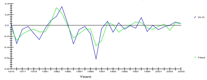
very close to the stylized value of one-third in the growth accounting exercises. The actual and

predicted values of output growth are shown below in Figure 1, which seems to be satisfactory.

Figure 1

Actual and Fitted Values of Dln y

DLYL

Fitted

Years

-0.2

-0.4

-0.6

-0.8 0.0 0.2 0.4

1975 1977 1979 1981 1983 1985 1987 1989 1991 1993 1995 1997 1999 2001 2003 2005

4.2. The Solow Model with JMLVECM

Although the endogenous variable bias is minimized by the instrumental variables method in

GETS, the Johansen systems method is more efficient compared to the single equations method

of GETS. However, GETS estimates are very useful for selecting the options in the

JMLVECM.5 Our earlier GETS estimates imply that the order of VAR could be two and that

both the intercept and trend may be retained in the selected VAR. One would get similar results

with the order selection routines for the VAR. The only uncertainty is whether the intercept and

trend should be constrained i.e., part of ECM or unconstrained i.e., outside ECM. Although this

choice does not matter for GETS estimates, they do in JMLECM. However, according to what

is known as the Pantula principle one should start with the unrestricted option first and if there is

no cointegration then the restricted option should be tried; see Harris and Sollis (2005).

5 Recently Sumner (2004) systematically outlined some difficulties in selecting the options in JMLVECM. However, Rao (2006) explains how GETS estimates can be used to select these options. This is not to say that

JMLECM is the best technique. In practice it is better to use alternative cointegration techniques to prepare

summaries of data for interpretation of the data. If alternative techniques yield similar summaries then our

Therefore, we have first used the unrestricted option and found one plausible cointegrating

equation between ln andlny kand the estimated cointegration equation is as follows:6

ln y = 0.535 ln k (4)

Equation 4 implies that the share of profit is 0.535, which is higher than 0.337 of GETS, but this

higher estimate is also plausible and the lower value in GETS may be partly due to some

residual endogenous variable bias. The JMLVECM parsimonious dynamic adjustment equation

for this version with the trend is as follows:

? lny = 2.24 - 0.02T - 0.525ECMt-1 -2.39? lnk t-1 -0.23DUM90

(4.96)* (-3.48)* (-4.91)* (-2.67)* (-1.94)** (5)

R bar2= 0.439; SER=0.137;

?2sc= 1.2359[.266]; ? 2

n=1.9869[.370] ? 2

ff=11.4778[.001]; ? 2

h=4.2993[.038]

* and ** indicate significance at the 5% and 10% level respectively.

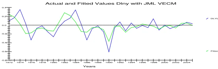
The result from the above JMLVECM baseline equation is satisfactory. Although the R bar

square is slightly less than the GETS equation, the actual and fitted values are reasonably good.

As in the GETS equation, the dummy variable recorded a negative coefficient of -0.253 and the

coefficient of trend is negative at -0.023 and are slightly differ from their GETS estimates. Thus

this equation also implies that technical progress in Kiribati has been negative. Moreover, the

coefficient of the error correction term in the JMLVECM is -0.53, which is similar to the ECM

in GETS of -0.72, meaning that convergence to equilibrium will also be smooth but slower. The

plot of actual and fitted values is in Figure 2.

6 In the eigenvalue and trace tests the null of no cointegration is rejected. The computed test statistics, with the

95% critical values in the brackets are respectively, 20.325 (18.33) and 28.235 (23.80). The null that there is at

least one cointegrating vector could not be rejected. The computed test statistics for these two tests are 7.91 (11.54)

and 7.91 (11.54).

5. Extension to the Solow Model

The next task here is to extend to the Solow model to capture the effects of the aforesaid three

shift variables viz., exports, aid and remittances. Using the GETS approach, the test is executed

on variables like export ratio, ratio of aid to GDP and remittance ratio (ratio of remittance to

employment) to examine whether they have any permanent and/or temporary effects on output.

To conserve space we shall not report all the details, as none of these variables are found to have

any meaningful positive permanent effects on output. These findings hold whether the GETS or

JMLVECM method is used, although often JMLVECM yielded implausible estimates for the

coefficient of ln k.7 To conserve space, we shall only report results with GETS using the

NLSQIV option in Mfit.

Figure 2

Actual and Fitted Values Dlny with JML VECM

DLYL

Fitted

Years

-0.2

-0.4

-0.6

-0.8 0.0 0.2 0.4

1972 1974 1976 1978 1980 1982 1984 1986 1988 1990 1992 1994 1996 1998 2000 2002 2004

5.1. GETS Result with the Export Ratio

The estimated parsimonious equation where the export ratio has only temporary effects on

output is as follows.

?l

ny

= 3.5 – 0.027T –0.66(lny

) + 0.41lnk

) + 0.44

? ln

y

+ -2.70

? ln

k

+

-0.27Dum90

(6.2)* (1.95)**

R bar2 =0.55, GR bar2 =0.493, Sargan's ?2 (4)=8.8668 [p=0.277];

?2ff = 2.8[0.094]; ? 2

n = 0.42[0.809].=4.42 [0.035]; ? 2

ff = 3.14 [0.076]; ? 2

n = 0.38 [0.83], ? 2

h =20.362[0.00].

* and ** indicate significance at 5% and 10% levels respectively. T-ratios are White adjusted.

Compared to the baseline equation, without the export ratio, this equation is very close in all

respects and only with minor changes to the estimated coefficients. The t-ratio of the adjustment

coefficient implies cointegration at the 5% level. The share of profits increased marginally to

0.41 from 0.337. It is noteworthy that the coefficient of ?lnEX is significant at only the 10%

level. This equation implies that a 10% increase in export ratio will increase growth in output

temporarily by about half a percent. Such low increase in output may be due to the fact that an

increase in exports does not significant backward and forward linkage effects in Kiribati.

When the JMLVECM approach is used, the null hypothesis of no cointegration is rejected at the

5% and 10% levels but the null of one cointegrating vector is not rejected. However, the

cointegrating vector showed that the coefficient of the export ratio is negative and the share of

profit is 5.4 which is meaningless. Therefore, there is no meaningful long run relationship

between the export ratio and output with this technique.

5.2. GETS Result with Aid

It is worth considering a GETS specification with aid, with linear and then a non-linear aid term

because non-linear terms are often found in some ad hoc specifications in which there are no

conditioning variables. However, only results with a linear aid term have been found to be

significant and the estimate is given below.

∆lny =2.93 – 0.04T – 0.73(lnyt -1

+

(1.28) (-4.31)* (5.56)* (1.96) (-2.46)*

+ 0.44∆lnyt-1 -3.69∆lnkt-2 -0.338Dum90 -0.31∆lnAID (7)

(3.36)* (-4.49)* (-3.53)* (-1.81)

R bar2 = .23981; GR-bar2 = .45515;SER = .14983; Sargan's ?2 (4) = 2.7161[.606]

?2sc = 4.6579[.031]; X 2

ff =3.1585[.076];? 2

n =.40260[.818]; ? 2

It can be seen that all the coefficients are significant although the share of profits are somewhat

high at 0.65. The t-ratio of the adjustment coefficient implies that there is cointegration only at

the 10% level. However, the effects of aid, in both long and short runs, are negative. It is

pointless to think about how large are these negative effects and our results partly support

Hughes (2003) concerns that aid has been unproductive in the Pacific Island Countries.

Estimation on the effects of aid was also executed with JMLVECM but none of the options

yielded any sensible results.

5.3. GETS Result with Remittances

GETS specifications with linear and non-linear remittance terms are estimated but the linear

specification gave better results although the coefficient of capital became insignificant.

Therefore, we re-estimated by constraining that the coefficient of capital is 0.337, which is the

estimate in the baseline equation. The following is the result.

?lnyt = 5.39 - 0.033T -0.83(lnyt -1 -0.337lnkt -1 -0.097lnREMt-1) + 0.41?lnyt-1

(5.97)* (-5.59)* (7.3)* (constrained) (4.6)* (-5.9)*

-0.38Dum90 -0.335?lnREMt (8)

(-5.99)* (-1.4)

R bar2=.48010;GR-Bar2 =.53615; SER =.12391; Sargan’s ?2 (4)= 6.918[.733]

?2sc=3.0260[.082]; X 2

ff=4.8827[.027]; ? 2

n=.50889[.775]; ? 2

h = 12.2192[.000].

The t-ratio of the adjustment coefficient implies cointegration at the 5% level. As can be noted

the long run effect of remittance is negative and significant. Although its short run effect is

negative it is insignificant. Therefore, we removed the short term effect and estimated the

equation. However, the coefficient of remittance in the ECM has become insignificant. We also

tried to estimate an equation in which remittance has only short run effect, but this equation was

unsatisfactory and although the coefficients of the changes in remittances were negative they

permanent effects. It is difficult to explain why remittances have permanent negative effects

unless, as the late Professor Kaldor once observed, in some countries people seem to prefer

leisure to work. In other words what is implied is that the labour supply curve in Kiribati is

perhaps backward bending.

5.4. Ad hoc Specifications

In order to get an idea of the nature of some ad hoc specifications without the two conditioning

variables, we have used JMLVECM to test the effects of aid with a few typical and simple ad

hoc specifications ignoring multiplicative terms.5

The assumed ad hoc specifications are: lny = a+b ln AID and lny = a+b ln AID +c ln AID2 .

Application of the JMLECM technique showed that w hile there was no cointegrating vector in

the linear specification, the trace and eigenvalue tests showed that there is one cointegrating

vector in the non-linear specification. Normalized on output, this cointegrating equation is:

ln y =21.918 ln AID -1.583 (ln AID)

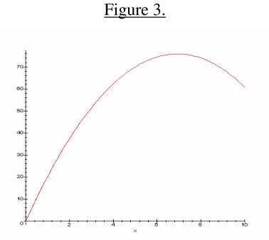
This implies that the maximum effect of aid per worker reaches when log of aid per worker is

about 7. The plot of this effect is given in Figure 3 below where x = log of aid per worker on the

horizontal axis and on the vertical axis its effect on output worker is shown.

Although this result looks impressive it should be noted that the implied elasticity of output per

worker with respect to aid per worker is implausibly high. In 2005 the value of log aid per

5 There are several other ad hoc specifications in which growth of output is simply regressed on aid etc and the

equation is estimated with OLS. We shall not examine all such ad hoc specifications. An elaborate specification to determine the effects of aid in a time series model is Fenny (2005)for the PNG in which it was found that aid has

no significant effect on growth. Although at times Fenny used 9 variables in the cointegrating vector, the two basic

worker is 5.5765 and the elasticity at this value is 4.27, implying that a 10% increase in aid will

cause about 43% increase in per worker output and such large effects of aid on output are

difficult to believe.

Figure 3.

Finally, we have included exports, aid and remittances along with capital per worker and used

JMLVECM to estimate a cointegration equation. Although we found one cointegrating

equation, the coefficient capital became negative. Therefore, we have tried to estimate an

equation with all these potential determinants of output with the NLLSQIV option and a GETS

specification. Due to severe multi-collinearity between the variables the estimation failed. When

the GETS specification is reestimated, without the instrumental variables method, the

coefficient of capital was negative. When this coefficient was constrained to its value in the

baseline GETS equation, the coefficients of exports, aid and remittances in the ECM term were

all insignificant. Furthermore, the residuals of this equation are found to be serially correlated

and therefore it is inappropriate to place any confidence in its summary statistics.

6. Conclusions

This paper explored the application of the Solow model and its extensions to Kiribati. In the

empirical results, the Solow model baseline equation from GETS and JMLVECM are found to

negative and significant coefficient of 0.27, a kind of downward intercept shift in the production

function due to increased inefficiency. Some possible reasons include: the failure of some

Government enterprises such as Te Mautari Ltd and low world copra price on copra production

and therefore low export earnings. Moreover, given the narrow export base, the trade deficit

escalated, meaning that Kiribati depends heavily on overseas countries for aid in food and other

consumer goods etc. Another noteworthy finding is that (based on the baseline results from the

GETS and the JMLVECM), the rate of TFP captured by the coefficient of trend is negative,

implying that Kiribati’s efficiency has declined at the rate of 2 to 3 per cent per year. The

implied profit share by the baseline GETS equation is plausible and very close to the stylized

value of one-third in many growth accounting exercises. The lack of managerial skills, closed

down businesses and unproductive investments, including the effect of brain drain are all

plausible reasons for the decline in efficiency in Kiribati.

In terms of the extensions to the Solow model, aid ratio and export ratio did not have any

permanent positive effects on output. In fact these two variables seem to have only permanent

negative effects, lending support to Hughes’ observation that aid has been counter productive in

PICs. The effects of aid from our estimates are thus contrary to the result with some ad hoc

specifications. However, the export ratio has a small temporary effect on output growth. aid

ratio has a negative short run effect on growth, A 10% increase in the export ratio will

temporarily increase per capita output by about 0.5. In conclusion, we may say that in Kiribati

output in the long run and its growth in the short run are essentially determined by capital

formation and therefore on investment.

There are a number of limitations in our study. For instance the available data on Kiribati cannot

be claimed to be reliable and our specifications and estimation technique are with a small

sample size. Therefore our study by and large is only exploratory. It is difficult to expect that

more reliable data on Kiribati and many other PICs will become available in the near future, our

Definitions and Data Sources

Y = Real GDP in 1991 prices

K = Capital stock estimated with the perpetual inventory method from data on total real

investment. Depreciation rate is assumed to be 5% and the initial capital stock is

assumed to be 1.2 times real GDP in 1970.

L = Employment in the formal sector

EX = Total exports divided by GDP

AID = Total foreign aid divided by employment

REM = Remittances made by Kiribati’s labour employed overseas including merchant ships

plus fishing license fees paid to Kiribati by overseas fishing trailers. It is measured in per

employed worker.

Sources:

All GDP data are from the UN database at http://unstats.un.org/unsd/snaama/selectionbasicFast.asp

Data on employment, aid and remittances are estimated by Toani Takirua from various

REFERENCES

Acemoglu, D., (ed.) (2004) Recent Developments in Growth Theory, London: Edward Elgar

Publishing.

Asteriou, D. and Price, S., (2004) Financial development and economic growth: Time series

evidence for the case of U.K., Discussion Paper No. 80, Department of Economics, City

University, London.

Ericsson, N. R. and MacKinnon, J. G., (2002) Distributions of error correction tests for

cointegration, Econometrics Journal, Vol. 5, pp. 285-318.

Fenny, S. (2005) The impact of foreign aid on economic growth in Papua New Guinea, Journal

of Development Studies, Vol.41, 1092 .1117

Gregory, A.W. and Hansen, B.E. (1996) “Residual-based tests for cointegration in models with

regime shifts,” Journal of Econometrics, Vol.70, .99-126.

Harris, R. and Sollis, R. (2005) Applied Time Series Modelling and Forecasting, Chichester:

John Wiley & Sons.

Hughes,H.,(2003) Aid Has Failed the Pacific? Issue Analysis No.33,Centre for Independent

Studies, Sydney.

Juselius, K. (1996) An empirical analysis of the changing role of the German Bundes Bank after

1983, Oxford Bulletin of Economic and Statistics, Vol. 58, 791-819.

Joyeux, J., (2007) “How to deal with structural breaks in practical cointegration analysis,” in

Rao, B. B. (ed.) Cointegration for the Applied Economist, Second Edition, Basingstoke:

MacKinnon, J. G. (1991) Critical values for cointegration tests,” in Engle, R. F. and Granger,

C.W.J. (eds), Long run Economic Relationships: Readings in Cointegration, Oxford: Oxford

University Press, pp.267-276.

Mankiw, N.G. Romer, D. and Weil, D., (1992) A contribution to the empirics of economic

growth,” Quarterly Journal of Economics, Vol. 107, 407-437.

Pesaran, M. H, Shin, Y. and Smith, R. (1996) Testing for the existence of a long run

relationship, DAE Working Paper No. 9622, Department of Applied Economics, University of

Cambridge.

Rao, B. B., (2006) Estimating short and long run relationships: A guide to applied economists’,

forthcoming, Applied Economics.

Rao, B. B and Rao, M. (2006) Exports and Determinants of Growth Rate: Some Evidence with

Time Series Data from Fiji, forthcoming, Applied Economics.

Rao, B. B., Singh, R and Fozia, N. (2006) An extension to the neoclassical growth model to

estiomate growth and level effects, Working Paper No. wp2006/4, School of Economics, the

University of the South Pacific.

Solow, R. M., (1956) A contribution to the theory of economic growth, Quarterly Journal of

Economics, Vol. 71, 65-94.

Sumner, M. (2004) A cautionary note on cointegration testing, Applied Economics Letters,

Vol.11, 275 .278

Turner, P. (2006) Response surfaces for an F-test for cointegration, Applied Economics Letters,