Multimoment Hydrodynamics in Problem on Flow around a Sphere: Entropy Interpretation of the Appearance and Development of Instability

http://dx.doi.org/10.4236/ojfd.2014.42015

Multimoment Hydrodynamics in Problem on

Flow around a Sphere: Entropy

Interpretation of the Appearance and

Development of Instability

Igor V. Lebed

Zhukovsky Central Institute of Aerohydrodynamics, Moscow, Russia Email: [email protected]

Received 31 March 2014; revised 30 April 2014; accepted 8 May 2014

Copyright © 2014 by author and Scientific Research Publishing Inc.

This work is licensed under the Creative Commons Attribution International License (CC BY).

http://creativecommons.org/licenses/by/4.0/

Abstract

Multimoment hydrodynamics equations are applied to investigate the phenomena of appearance and development of instability in problem on a flow around a solid sphere at rest. The simplest solution to the multimoment hydrodynamics equations coincides with the Stokes solution to the classic hydrodynamics equations in the limit of small Reynolds number values,

Re



1

. Solution

0

Sol to the multimoment hydrodynamics equations reproduces recirculating zone in the wake

behind the sphere having the form of an axisymmetric toroidal vortex ring. The Sol0 solution remains stable while the entropy production in the system exceeds the entropy outflow through the surface confining the system. The passage of the first critical value Re0

∗ _{is accompanied by the}

0

Sol solution stability loss. The Sol0 solution, when loses its stability, reproduces periodic pul-sations of the periphery of the recirculating zone in the wake behind the sphere. The Sol1 and

2

Sol solutions to the multimoment hydrodynamics equations interpret a vortex shedding. After

the second critical value Re0

∗∗ _{is reached, the}

0

Sol solution at the periphery of the recirculating

zone and in the far wake is replaced by the Sol2 solution. In accordance with the Sol2 solution, the periphery of the recirculating zone periodically detached from the core and moves down-stream in the form of a vortex ring. After the attainment of the third critical value Re0

∗∗∗_{, the}

2

Sol

path to depart from the state of statistical equilibrium. Having lost the stability, the system does not reach a new stable position. Such a scenario differs from the ideas of classic hydrodynamics, which interprets the development of instability in terms of bifurcations from one stable state to another stable state. Solutions to the multimoment hydrodynamics equations indicate the direc-tion of instability development, which qualitatively reproduces the experimental data in a wide range of Re values. The problems encountered by classic hydrodynamics when interpreting the observed instability development process are solved on the way toward an increase in the number of principle hydrodynamic values.

Keywords

Multimoment Hydrodynamics, Instability, Entropy, Vortex Shedding

1. Introduction

Detailed evaluating the results of the direct numerical integration of the Navier-Stokes equations against expe-riment in problem on flow past a hard sphere at rest is carried out in [1]. Experiment records three stable me-dium states. Each of these three stable flows begins to develop in its own direction, qualitatively different from other flows when it loses stability. Calculation satisfactory reproduces all three stable medium states observed experimentally. However, the calculation is incapable of producing anything that corresponds to seven unstable regimes observed along the three directions of instability development. The analysis of numerous divergences between the results of numerical integration of the Navier-Stokes equations and the experiment [1]-[3] led to the following conclusion. Solutions to the classic hydrodynamics equations successfully reach the border of the in-stability field represented by the dashed slanting line in Figure 1 from [3]. As Reynolds number grows, these solutions move along the border of the field. However, the solutions to the classic hydrodynamics equations are unable to cross this border and to pass into the instability field.

The Navier-Stokes equations themselves are called as the most probable reason for discrepancies between calculation and experiment [1]-[4]. It may be likely that the Navier-Stokes equations become inapplicable to un-stable phenomena. The responsibility for the failure of the classic hydrodynamics was laid on the approximation made in deriving the Boltzmann equation, namely, the hypothesis of molecular chaos “Stosszahlansatz”. The Boltzmann hypothesis closes the kinetic equation, allowing classic hydrodynamics to be constructed for only three lower principle hydrodynamic values. It turns out that the neglect of higher principle hydrodynamic values does not introduce visually observable changes into the picture of stable flows. This error, however, grows very rapidly after the loss of stability.

In present paper the multimoment hydrodynamics equations [5] are applied to solve a problem on flow past a hard sphere at rest at a wide range of Re values. The direction of evolution of the ground axisymmetric flow

( )

0

exp

U x [1] after losing its stability is studied. In Section 2, the problem is formulated. In Section 3, the prob-lem is solved for the Stokes flow around a sphere, i.e., at Re1. The Section 4 is devoted to construction of the Sol₀ solution to the multimoment hydrodynamics equations suitable of interpreting the stationary axisym-metric flow at a moderately high Re values. The Section 5 examines the behavior of the Sol0 solution that loses its stability after the passage of the first critical Reynolds number value Re∗₀. In Section 6, the characteris-tic features of the appearance of instability are interpreted in terms of entropy. The principle of retention and loss of the open system stability is formulated. In Section 7, the characteristic features of the development of in-stability are interpreted in terms of entropy. The evolution criterion is formulated. The Section 8 is devoted to finding the solutions to the multimoment hydrodynamics equations capable of reproducing a vortex shedding. The Section 9 provides an algorithm to select one unstable solution of many found unstable solutions. The se-lected solution indicates the direction of system evolution. In Section 10, the results are compared with the ex-perimental data.

2. Problem Statement

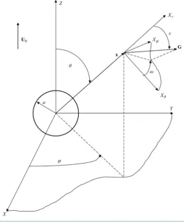
moves in gas at constant velocity U₀ along the Z₀ axis of the immobile Cartesian frame of reference 0 0 0

X Y Z . Let us now pass from X Y Z_{0 0 0} to the Cartesian frame of reference XYZ with the axes parallel to

those of X Y Z_{0 0 0} and the origin made coincident with the center of the moving sphere. In the XYZ frame of reference, the sphere is at rest, the inflowing-gas velocity at an infinite distance from the sphere, U₀, is aligned with the positive direction of the Z axis, and the flow problem is stationary.

The pair distribution function f_p( )0

(

G v₀, ₀

)

corresponding to the equilibrium state is

( )0

₍

₎

0 3 2 3 2 20 20

0 0

0 0 0 0

, exp

2 2π 2π 2 2

p

n M M

f

kT kT kT kT

µ

µ  

   

= _{    }− − _

     

G v

G v (2.1)

where n₀ and T₀ are the local density of the number of particles and the temperature of unperturbed gas,

2

M = m, µ =m 2, m is the mass of a gas particle, and G₀ and v₀ are the velocity of the center of mass and relative velocity of the pair of particles. In XYZ, the pair distribution function f_p

(

x G, ,v

)

can be written as

(

)

( )0

₍

₎

₍

₎

, , , , ,

p p p

f x G v = f G v + ∆f x G v

( )0

₍

₎

3 2 3 2

(

0

)

2 2

0

0 0 0 0

, 2π exp

2π 2π 2 2

p

M

M v

f v n

kT kT kT kT

µ

 −

µ



    _{ }

=     − −

 

    _{ }

G U

G (2.2)

0 0 0 v

= + = =

G G U v v v

[image:3.595.166.431.377.697.2]

Let x y, , and

z

be the Cartesian coordinates of point

x

in the space; ,rθ, and

ϕ

are its spherical coor- dinates, x=rsin cos ,θ ϕ y=rsin sin ,θ ϕ and z=rcos

θ

, Figure 1. Bring the origin of the Cartesian frame of

Figure 1. The XYZ frame with its origin at the center of the sphere. The

r

reference X Y Z_r θ ϕ into coincidence with point

x

so that the Xr axis is directed along

x

vector. Mark the projections of vector G onto the XYZ axes by G G_x, _y, and G_z, its projections onto the axes of X Y Z_r θ ϕ, by G Gr, θ, and Gϕ, and its spherical coordinates, by G,ε, and ω, Figure 1.

The basic property of pair distribution functions (17) from [3] is that fp

(

t, , ,x G v

)

is conserved with time

along the trajectory of the center of mass of a pair of particles. In the stationary case, the fp

(

x G, ,v

)

function

remains unchanged along a straight line parallel to vector G

(

, ,

)

0

p

f v

∂

= ∂

x G G

x (2.3)

The Fxy=G yx −G xy , Fzx =G x G zz − x , and Fzy =G yz −G zy functions are the first integrals of Equation

(2.3). These functions were termed in [6] trajectory invariants. In this study, consideration is restricted to gas flows around a sphere, which are invariant under rotation through an arbitrary angle

ϕ

about the Z axis. Let us compose combinations of trajectory invariants Fxy, Fzx, and Fzy, invariant with respect to this rotation

F_xy = −G_rsin sin sinθ ε ω

(

)

2

(

2

)

Ф_z = − G_xF_zx+G_yF_zy =G r cos sinθ ε+sin cos sin cosθ ε ε ω (2.4)

(

)

1 2

2 2 2

Фr = Fxy+Fzx+Fzy =Grsin

ε

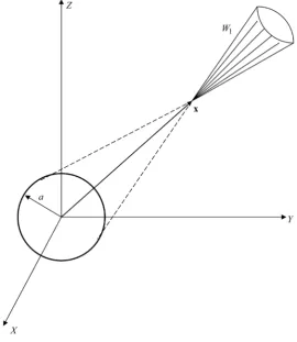
[image:4.595.163.434.398.710.2]

By virtue of the flow geometry, there are two independent regions of integration with respect to G at each point

x

in the gas. The first region, denote it by W₁, is a spherical cone, Figure 2. This region incorporates the trajectories of centers of mass of pairs of particles that originate and terminate at the surface of the sphere. The integration limits for this group of trajectories are 0≤ ≤ ∞ ≤ ≤G , 0

ω

2π, 0≤ ≤

ε

arcsin

( )

a r . The second region, W₂, embraces all possible trajectories of centers of mass of particle pairs converging to point

x

. The integration limits for the second group of trajectories are unbounded.

According to the general approach to solving the multimoment hydrodynamic equations in terms of pair func-tions, outlined in [6], solution ∆fp

(

x G, ,v

)

is sought for in the form of an infinite series of the products of

tra-jectory invariants (2.4)

(

)

(

)

3 2 3 2

2 2

0 0 0

0 0 0 0

, , 4π exp , Ф Ф F

2π 2π 2 2

k l m n

p klmn z r z xy

k l m n

M M v

f v c v G

kT kT kT kT

µ µ +∞ +∞ +∞ +∞

= =−∞ = =

     

∆ = _{    }− − _

     

∑ ∑ ∑ ∑

G

x G G (2.5)

The spatial dependence of ∆fp

(

x G, ,v

)

(2.5) is controlled by trajectory invariants (2.4), and coefficients

klmn

c are independent of

x

. In keeping with definitions given in [5], the expressions for the principal hydrody-namic values—the moments of fp

(

x G, ,v

)

(2.2)—can be written as

0

1 1

d 2n=2n + ∆

∫

fp g,

0 0

1 1

d 2nUi= 2n U i+

∫

G fi∆ p g,

2

0 0

3 3

d

4 4 2

v

p v

p = n kT +

∫

µ ∆f g (2.6)

2

2 2

0 0 0 0

3 3 1 1 3 3

, d

4 4 4 4 4 4 2

G G G

p MG

p = s + Mn U − MnU s = n kT +

∫

∆f g, v v

p =nkT , pG =nkTG,

0 0 0 0 0

1 1 1 1

, d

2 2 2 2 2 2

G G G

ij ij i j i j ij ij i j p

P =1S +1Mn U U − MnU U S = n kTδ +

∫

MG G∆f g, ,

G G G G G G

ij ij ij ij ij ij

p =P −p δ s =S −s δ ,

2

0 0 0

1 3 1 3 1

, d

2 4 2 4 2 2

v v v v i

i i i i i p

G v

q = n kT U + Q − p U Q =

∫

µ ∆f g,

2

2 2

0 0 0 0 0 0

1 5 1 1 5 1

, d

2 4 4 2 4 2 2

G G G G G i

i i i i i ki k i i p

MG G q = n kT U + Mn U U + Q − p U −1p U −1MnU U Q = ∆f

2 4

∫

g

Here, n is the local density of the number of particles; U is the hydrodynamic velocity; G

p ,

T

G, G

ij

P , and G

q are the pressure, temperature, stress tensor, and heat flux corresponding to motion of the centers of mass of pairs of particles; v

p ,

T

v, and v

q correspond to relative motion of particles within pairs; 2

d =g v vd dG. Nonprincipal hydrodynamic values v

ij

p and Gv

q are given by Equation (21) from [3] with the Navier- Stokes accuracy. In terms of spherical coordinates, these values for cylindrically symmetric flows considered in this study (i.e., for flows invariant with respect to rotation through an arbitrary angle

ϕ

about the Z axis) assume the form

4 4

2

3 3

v v

v r r v r

rr v v

U q Q

p

r p r p r

η η

η∂ ∂ π ∂

= − − + = − ∂ ∂ ∂    4 4 2 3 3 v v v v

v r r v r

v v

U q Q

U q Q

p

r r p r r p r r

θ θ θ

θθ η _θ η _θ π η _θ

    ∂ ∂ ∂   = −  + _∂ −  + _∂ + = −  + _∂          

ctg 4 ctg 4 ctg

2

3 3

v v

v v

v r r v r

v v

U q Q

U q Q

p

r r p r r p r r

θ θ θ

ϕϕ

θ η θ η θ

η    π  

= − _ + _−  + + = −  +         2 2 3 3

v v v v

v r r r

r v v

U U q q Q Q

p r r r

r r r p r r r p r r r

θ θ θ

ϕ η _θ η _θ η _θ

         ∂   ∂  ∂ ∂ ∂ ∂ = −  _∂  + _∂ −  _∂  + _∂ = −  _∂  + _∂                     2 4 div div 3 9 v v v p η η

(

)

2 2

5

sin sin

4 4 sin

ctg

3 2

4 3

v G v G

Gv rr r

r v

v

G G v r v v r v v r v v

r r r r

v v

kT p kT p

kT

q r r

r m p r r m m

U U U U

U U U

kT

p p q q q q q q q

m r r r r r r r

p r p

θ

θ θ θ θ

θθ ϕϕ θ θ θ

η η _{θ θ}

θ θ θ η η θ θ      ∂   ∂ ∂ = − _∂ _ _− _∂  +_∂          ∂ ∂ ∂ ∂   + + − _ + + + + + − _ ∂ ∂ ∂ ∂      

(

)

2 2 5 sin sin

4 4 sin

ctg

3 4

4 3

v G v G

Gv r

v

v

G G v v r v v r v v r v

r r r r

v v

kT p kT p

kT

q r r

r m p r r m m

U U U U U U U

kT

p ctg p q q q q q q q

m r r r r r r r

p r p

θ θθ

θ

θ θ θ θ

ϕϕ θ θ θ θ θ

η η _{θ θ}

θ θ θ

θ

η _θ η

θ θ      ∂   ∂ ∂ = − _∂ _ _− _∂  +_∂          ∂ ∂ ∂ ∂   + − − _ + + + + + − _ ∂ ∂ ∂ ∂      

Here,

η



is the coefficient of the dynamic viscosity. From the definitions of gas pressure p, temperature T, viscous stress tensor p_ij, and heat flux q [5] itfollows that they are linear combinations of moments (2.6) and (2.7)

5

2 2 2 2 6

G v G v G v G v

ij ij i i Gv

ij i i

p p q q

p p T T

p= + T = + p=nkT p = + q = + +q (2.8) According to [5], the overall equations of conservation of the number of particles, momentum, and energy assume the form

0 i i nU n t x ∂ ∂ _{+ =}

∂ ∂ (2.9)

1 0 2 G ij v i i j S nU

t m x

∂ 

∂

+ _ + ∏ =_

∂ _∂ _ (2.10)

5

3 3

0

4 4 2 6 2

G v

G v Gv

i i i Q Q s p t x    

∂ _{+ +} ∂ _{+ +}Λ ₌

 

 

∂ _{ } ∂ _{ } (2.11)

The basic property of pair distribution functions (17) from [3] subdivides Equations (2.10) and (2.11). As re-cast in terms of the spherical coordinates, the ∏v_i and

Λ

Gv components assume the following form for the cy-lindrically symmetric flow in question

1

2 ctg 0

v v v

v rr r v v v v

r rr r

p p p

p p p p

r r r r

θ

θθ ϕϕ θ

θ

θ

∂ ∂

∂ _{ }

Π = + + + _ − − + _=

∂ ∂ ∂

(

)

1

ctg 3 0

v v v

v r v v v

r

p p

p

p p p

r r r r

θθ θ

θ

_θ

_θ

θθ ϕϕ

θ

θ

∂ ∂

∂ _{ }

Π = + + + _ − + _=

∂ ∂ ∂ (2.12)

(

)

(

)

2 2

1

sin 2 sin 2 0

sin

Gv Gv v v Gv v v

r r rr r r r

r q U p U p r q U p U p

r

r

θ

θ

θ θ

θ

θ

θ θ θ θθ

∂ ∂

 _{   }

Λ = _{ } + + _+ _ + + _=

∂ ∂

  (2.13)

The boundary conditions must allow for the fact that the contribution of the ∆fp

(

x G, ,v

)

function given by

Equation (2.5) to the hydrodynamic values vanishes at an infinite distance from sphere

(

, ,

)

0

p _r

f v

→∞

∆ x G → (2.14) At the surface of the sphere, i.e., at r=a, one has to impose the no-leak and no-slip conditions

0 0

r r a r a

nU ₌ = nU_{θ =} = (2.15) Heat flux q_r traversing each element of the sphere surface must be counterbalanced by the heat flux within the sphere q_rcond and the thermal radiation ∆E

(

cond

)

r r a r _{r a}

q ₌ q E

=

(

0

)

cond r

T

q E T T

r

γ ∂ σ

= − ∆ = −

∂

Here,

γ

is the coefficient of the thermal conductivity of the sphere, and σ is the coefficient of the sphere emissivity.

3. Flow around a Sphere at Small Re

Let us formulate dimensionless parameters Ma2=mU02 kT0, where Ma denotes the Mach number, and the Reynolds number Re=2mn U a_{0 0} η₀,

η

0=

η



( )

T0 . Multimoment hydrodynamics Equations (2.9)-(2.13) will be brought to a dimensionless form in a conventional manner [7]. It turns out that the dimensionless equations contain Ma2 and Re. Hydrodynamic values can be represented as parametric series

( )

2

( )

( ), ( ),

0 0

0 1 0 1

ˆ

Ma k Rel k l k l

k l k l

F F F F F

∞ ∞ ∞ ∞

= =− = =−

=

∑ ∑

=

∑ ∑

 (3.1)

Here, F=F

( )

x sequentially assumes values n x

( )

; n x U x

( ) ( )

; _pv

( )

_{x , s}G

( )

_{x , and} G

( )

ij

s x ; _QG

( )

_x

and _Qv

( )

_{x , and}

0

F sequentially assumes values n₀; n U_{0 0}; n kT_{0 0}; n kT U_{0 0 0}. Symbols  and



appear over dimensionless quantities. Multimoment hydrodynamics Equations (2.12), (2.13) are written with the Navi-er-Stokes accuracy, by which token expansion (3.1) contains no terms with l≤ −2.

Consider the flow regime at small Reynolds number Re1. At the hydrodynamic stage of description cha-racterized by small values of the Knudsen number Kn1, Ma∼Kn Re⋅ 1. Terms of the order of

2 0 0Ma Re

n kT dominate expansion (3.1) of the second-order moments pv and G

( )

ij

S x in the flow regime in question. In expansions (3.1) of hydrodynamic values n, pv, and G

ij

S , it will suffice to retain only (1, 1) (1, 1)

, v

n − p − , and S_ijG(1, 1−), respectively. Expansion (3.1) of the particle density flux nU is reasonably be re- stricted to

( )

 ( )

0,0

nU , which provides for the n kT_{0 0}Ma2 Re desired order of the terms in Equation (2.7) for

v ij

p . As noted in [6], the Navier-Stokes approximation is not accurate enough to calculate temperature compo-nents TG(1, 1−) and Tv(1, 1−). Thus, at Re1, the spatial dependence of temperature is neglected.

Let us truncate expansion (2.5) to the three lowest-order terms

( )0

₍

₎

3 2 3 2 2 2

{

1 2

}

1 2 3

0 0 0 0

, , 4π exp Ф Ф Ф

2π 2π 2 2

p z r z z r

M M v

f v c G c c G

kT kT kT kT

µ µ −

     

∆ = _{    }− − _ + +

     

G

x G (3.2)

1 1 100 2 0010 3 1200

c =c₋ c =c c =c

Each of three terms of series (3.2) can contribute to each principal hydrodynamic value (n, nU, pv, sG,

G ij

s , qv, and qG). Considering that the principal hydrodynamic values are linearly independent, coefficients

, 1, 2, 3

i

c i= , of expansion (3.2) can be written as linear combinations of six arbitrarily chosen components ( )

₍

₎

( ) ( )

2 2

, ,

,

, 0 0

,

2 2

r s

k l k l

i i i r s

r s

MG v

c c v c

kT kT

µ

   

= = _{   }

   

∑

G (3.3)

To calculate the hydrodynamic values (2.6), the first component of series (3.2) has to be integrated with re-spect to G with the appropriate weight function of velocities G and v within region W₂, and the second and third components, within region W₁. Why ∆f_p( )0 is approximated by Equation (3.2), and its components are integrated in such a way is explained below. The integration yields

3

0 0cos 2 1cos 2 2cos 3 r

a a

nU n U A A

r r

θ

θ

θ

= + + ( )0,0

1 0 0ˆ1 A =n U A

3

0 0sin 1sin 2sin 3

a a

nU n U A A

r r

θ = −

θ

−

θ

+

θ

A2 =n U A0 0ˆ2( )0,0 (3.4) 2

0 2 3cos 2

a

n n A

r

θ

= + 2 (1, 1)

3 0 3

Ma _ˆ Re A =n _ _A −

2

0 0 2 3 0cos 2

v a

p n kT D kT

r

θ

= + 2 (1, 1)

3 0 0 0 3

Ma _ˆ Re D kT =n kT _ _D −

 

2

0 0 4 3 0cos 2

G a

s n kT B kT

r

θ

= + 2 (1, 1)

3 0 0 0 3

Ma _ˆ Re B kT =n kT _ _B −

 

2 4

3 0 2 4

8 cos

G rr

a a s B kT

r r

θ 

=  − 

 

2 4

3 0 2 4

4 cos

G G a a

s s B kT

r r

θθ ϕϕ θ

 

= = −  − 

 

4

3 0 4

4 sin

G r

a

s B kT

r

θ = −

θ

Here, ( ) ( ) ( ) ( ) ( ) ( ) 1 2

0,0 0,0 0,0

0

1 1 0,0 1 1,0 1 0,1

2

π 3

2

2 π 2

kT

A c c c

a M     = _{  } + + _    ( ) ( ) ( ) ( ) ( ) ( ) ( ) ( ) ( ) ( ) ( ) ( ) 3 2

0,0 0,0 0,0 0,0 0,0 0,0

0

2 2 0,0 2 1,0 2 0,1 2 2,0 2 3,0 2 1,1

2

π 3 9

3 12 60

2 π 2 2

kT a

A c c c c c c

M     = _{  } + + + + + _    ( ) ( ) ( ) ( ) ( ) ( ) ( ) ( ) ( ) ( ) ( ) ( ) 3 2 2

1, 1 1, 1 1, 1 1, 1 1, 1 1, 1

0

3 3 0,0 3 1,0 3 0,1 3 2,0 3 3,0 3 1,1

2

π 3 9

3 12 60

2 π 2 2

kT a

A c c c c c c

M

− − − − − −

   

= _{  } + + + + + _



  (3.5)

( ) ( ) ( ) ( ) ( ) ( ) ( ) ( ) ( ) ( ) ( ) ( ) 3 2 2

1, 1 1, 1 1, 1 1, 1 1, 1 1, 1

0

3 3 0.0 3 1,0 3 0,1 3 2,0 3 3.0 3 1,1

2

π 3

4 20 120 6

2 π 2

kT a

B c c c c c c

M − − − − − −     = _{  } + + + + + _    ( ) ( ) ( ) ( ) ( ) ( ) ( ) ( ) ( ) ( ) ( ) ( ) 3 2 2

1, 1 1, 1 1, 1 1, 1 1, 1 1, 1

0

3 3 0,0 3 1,0 3 0,1 3 2,0 3 3,0 3 1,1

2

π 5 15

3 12 60

2 π 2 2

kT a

D c c c c c c

M − − − − − −     = _{  } + + + + + _    ( ) ( ) ( ) ( ) ( ) ( ) ( ) ( ) ( ) ( ) ( ) ( )

1 2 3 2 3 2

2

0,0 0,0 0,0 0,0 1, 1 1, 1

0 0 0 0 0

1 , 1 , 2 , 2 , 3 , 2 3 ,

0 0 0

1 2 Ma

ˆ ˆ ˆ

Re

r s r s r s r s r s r s

M M M

c a n U c c n U c c n c

kT a kT a kT

− −

       

= _{ } = _{ } = _{   }

 

     

The order of coefficients A₁ and A₂ appearing in Equations (3.4, 3.5) depends on the only density flux component,

( )

 ( )

0,0

nU , retained in expansion (3.1) at Re1. The order of coefficients A₃, B₃, and D₃ de- pends on components (1, 1) (1, 1)

, v ,

n − p − and S_ijG(1, 1−) of expansion (3.1). Using one of six linear combinations of coefficients

c

( )_{2 ,}0,0_{( )r s} , we eliminate the contribution to the particle density n, proportional to n₀Ma, which is missed in expansion (3.1). Using two linear combinations of coefficients

c

_{2 ,}( )_{( )}0,0_{r s} , we eliminate the contribution to pv and sG that is proportional to n kT_{0 0}Ma and is missed in expansion (3.1). Two other linear combina- tions of

c

_{2 ,}( )_{( )}0,0_{r s} enable us to eliminate the contribution to qv and qG that is proportional to n kT U_{0 0 0}. The reason why qv and qG contain no terms proportional to n kT U_{0 0 0} will be elucidated in Section 4. The last, sixth linear combination of

c

₂( )0,0_{( )r s,} yields A₂ in Equation (3.5). Three linear combinations of

c

_{3 ,}(1, 1_{( )r s}−) enable us to eliminate the contribution to nU being proportional to n U_{0 0}Ma Re and the contribution to qv and qG

being proportional to n U kT_{0 0 0}Ma Re, which are missed in Equation (3.1). The first term of series (3.2) con- tributes only to the first and thethird moments of the fp

(

x G, ,v

)

function. Two linear combinations of ( )

( )0,0 1 ,r s

c

offer means of eliminating the contribution to qv and qG being proportional to n kT U_{0 0 0}.

Using boundary conditions (2.15) we obtainAˆ₁( )0,0 = −3 4, Aˆ₂( )0,0 =1 4. The components of tensor v

( )

ij

p x (2.7) can be determined from Equation (3.4). Substituting v

( )

ij

p x and _pv

( )

_{x from (3.4) into any of the}

( )1 1 ( )1 1 ( )1 1

ˆG ˆv ˆ

s − = p − = p − , hence, Bˆ₃(1, 1−) = −3 4, Aˆ₃(1, 1−)= −3 2. Substituting the foregoing expressions for the coefficients Aˆ₁( )0,0 , Aˆ₂( )0,0 , Aˆ₃(1, 1−), Bˆ₃(1, 1−), Dˆ₃(1, 1−) into Equation (3.4) and using definitions (2.8), we obtain



( )

( )0,0 3

0 0 0 0 3

3 cos 1

2 2

r

a a n U nU n U

r r

θ 

= _ − + _

 



( )

( )0,0 3

0 0 0 0 3

3 sin 1

4 4

a a n U nU n U

r r

θ θ

 

= _− + + _

  (3.6)

(1, 1) 0 0 2

(

(1, 1)

)

0 2 0

0

3

cos 1

2

U a

n n n n n

akT r

η _θ

− _{= −}  _{= +} −

 

(1, 1) 0 0 2

(

(1, 1)

)

0 0 2 0 0

3

cos 1

2

U a

n kT p p n kT p

a r

η

_θ

− _{= −}  _{= +} −

  _(3.7)

(1, 1) 0 0 2 4

0 0 2 4

3

cos

rr

U a a

n kT p

a r r

η _θ

− _{= −}  ₋ 

 

 



 (1, 1) 0 0 4

0 0 4

3 sin 2

r

U a

n kT p

a r θ

η

θ

− ₌  

(1, 1) (1, 1) 0 0 2 4

0 0 0 0 2 4

3

cos 2

U a a

n kT p n kT p

a r r

θθ ϕϕ η _θ − ₌ − ₌  ₋      

  ( )1 1

0 0

ij ij

p =n kT p −

Distributions (3.6), (3.7) follow from the classic hydrodynamics equations [7] for the Stokes flow, which are identical to the multimoment hydrodynamics equations in the limit Re1 [6].

The hydrodynamic values (3.6), (3.7) assume the form of a linear combination of the products of

( )

a r k by trigonometric functions. To calculate (3.6), (3.7), the first component of Equation (3.2) was integrated with re-spect to G within the W₂ region, and the second and third components, within the W₁ region. If, on the contrary, the first component is integrated within W₁, and the others, within W₂, Equation (3.4) contain the products of irrational

(

1−a2 r2

)

k+1 2 and trigonometric functions. However, with such products in Equation (3.4), it is impossible to satisfy boundary conditions (2.15) and equations of momentum conservation (2.12) si-multaneously. When the higher-order terms are being retained in expansion (2.5), the functions will appear in Equation (3.4) which are nonlinear in cosθ and sinθ and the Equations (2.15) and (2.12) cannot, as previously, be satisfied simultaneously.

4. Stationary Flow around a Sphere at Moderately High Re

Consider a flow at a moderately high Re and Ma21. In this case,

( )

 ( ) 0,0

nU will be retained together with two othercomponents of expansion (3.1) of the flow density nU:

( )

 ( )

0,l1

n

+

U and

( )

 ( )

1,l

nU ,

l

=

0,1,



.

In ad- dition to already obtained components of expansions (3.1) of the zero- and second-order moments of the fp

(

x G, ,v

)

pair distribution function, ( )k l,

n , v k l( ),

p , and S_ijG k l( ), with

k

=

0,1

и

l

=

0,1,



, will be taken into account. Expansions (3.1) of the energy fluxes _QG _{and Q}v _{will be limited to} G k l( ),

Q and Qv k,l( ) with

k

=

0,1

и

1, 0,

.

l

= −



Expressions for hydrodynamic values (2.6) will be constructed by the same principle as in Section 3—as li-near combinations of the products of

( )

a r k and trigonometric functions. This principle governs both the structure of the retained terms of expansion (2.5) and the region of integration with respect to G for each term of expansion (2.5). In addition to three terms given by Equation (3.2), the following components of expansion (2.5) will be included

( )1

₍

₎

( )1,0

₍

₎

( )1,1

₍

₎

, , , , , ,

p p p

f v f v f v

∆ x G = ∆ x G + ∆ x G

( )

₍

₎

{

}

3 2 3 2

2 2

1,0

0 0 0 0

1 2 1 3 2 1 1

4 5 6 7 8 9 10

, , 4π exp

2π 2π 2 2

Ф Ф Ф F Ф Ф Ф Ф

p

r z r r xy z z r z z z r z

M M v

f v

kT kT kT kT

c c G c c G c G c G c G

µ µ − − − − −       ∆ = _{    }− − _       × + + + + + + G x G (4.1)

4 0 100 5 2 100 6 0 302 7 1000 8 1 100 9 1010 10 1 110

( )

₍

₎

{

}

3 2 3 2 _{2 2}

1,1

0 0 0 0

1 3 1 2 2 1

11 12 13 14 15

2 2 1 4 4 1 4

16 17 18 19 20 21

, , 4π exp

2π 2π 2 2

Ф Ф Ф Ф Ф Ф

Ф Ф Ф

p

z r z r z z z z r z z z r z z r z r

M M v

f v

kT kT kT kT

c G c G c c G c G

c c G c G c G c G c G

µ µ

− − −

− −

     

∆ = _{    }− − _

     

× + + + +

+ + + + + +

G x G

(4.2)

11 1 100 12 3 100 13 0010 14 2010 15 2 110 16 0000

c =c− c =c− c =c c =c c =c− c =c

17 2000 18 2 100 19 4000 20 4 100 21 4100

c =c c =c− c =c c =c− c =c

Generally, each component of expansions (4.1, 4.2) contributes to each principle hydrodynamic value, irres-pective of the order of terms retained in expansion (3.1). Considering that the principle hydrodynamic values are linearly independent, each coefficient c ii, =4,, 21, should be represented as series (3.3) of six terms for any

considered order of expansion (3.1). Function ∆f_p( )1,0 given by (4.1) is used to calculate the zero- and the second-order moments. The contribution of ∆f_p( )1,0 is eliminated from the first- and third-order moments through the use of Equation (3.3), as in Section 3. Function ∆f_p( )1,1 (4.2) is used exclusively to calculate the first- and the third-order moments. The terms of Equation (4.1) proportional to c₄, c₅, c₆ and the terms of Equation (4.2) proportional to c₁₁, c₁₂ are integrated with respect to G within region W₂. The terms of Equation (4.1) proportional to c₇,,c₁₀ and the terms of Equation (4.2) proportional to c₁₃,,c₂₁ are inte-grated with respect to G within region W₁.

Distributions of the principle hydrodynamics values (2.6) are given in [8] by Equations (A.1)-(A.7). The ex-pressions (A.1)-(A.7) are written in terms of coefficients C ii, =1,, 50. Coefficients Ci are expressed in terms of c ii, =4,, 21 which appear in Equations (4.1), (4.2). Each coefficient ci is expanded into series (3.3) of six r s, −terms for each considered

k l

,

−

order of expansion (3.1). In what follows, the relationships between C_i and c_i required to derive explicit expressions for ∆f_p( )1,0 and ∆f_p( )1,1 , will be omitted. Each coefficient C ii, =1,, 50, contains dimensionless multiplier Cˆi.

In order to calculate C iˆ ,_i =1,, 50, one needs, as in Section 3, to satisfy boundary conditions (2.14)-(2.16) and equations of conservation (2.12), (2.13). Imposing boundary conditions (2.15) upon the particle density flux

nU (A.5) from [8], we express 16 coefficients Cˆ_i, i=34,, 44, 46,, 50 in terms of 34 remained coeffi-cients [8]. As revealed in [6], the _{0 0 0}Ma Re2 l 1

n kT U − -order approximation to the total energy-flux vector Q

(

l=0,1,

)

is

2 *

0 * 0 0 0 0

1

5 2 2

G _{G v}

ij i

i i i

i j

s mn U U

T s p

Q Q T Q

x nk x n

λ∂ ∂  +

= −  + + = =

∂ ∂

 

 

 (4.3)

Here

λ

=15k

η

 4m is the coefficient of the thermal conductivity. Substituting the expressions for hydrody-namic values (A.1)-(A.4) from [8] into Equation (4.3), it is possible to express 8 coefficients Cˆ_i, i=26,, 33, in terms of 26 remained coefficients. Substitute Equations (A.2), (A.5), and (A.6) from [8] into equation of mo- mentum conservation (2.12) and equate the coefficients of the

( )

a r kcosnθsinmθ products for either of the orders, n kT_{0 0}Ma2 a and n kT_{0 0}Ma4 aRe. Then 6 coefficients Cˆ_i, i=21,, 25, 45, can be expressed in terms of 20 remained coefficients Cˆ_i, i=1,, 20, [8]. Eventually, the expressions for the principle hydrody-namic values (2.6) can be written as

( ) ( )

(

1, 1 1

)

( )1 ( )1, 0

0

1 l

l

n n n n n n

∞ −

=

= + +  =

∑

 (4.4)

( )1 2

_{( )}

(

2

)

_{( )}

(

2

)

_{( )}

3

_{( )}

_{( )}

2

1 2 3 4

ˆ ˆ ˆ ˆ

Ma 1 2 cos 1 3cos 1 2 cos

n = _− C θ+ a r −C θ− a r − C a r −C θ a r _

(1, 1) (1) (1) (1, )

0 0

0

(1

)

v v v v v l

l

p

n kT

p

p

p

p

∞ −

=

=

+



+





=

∑



(4.5)

( )1 2

(

2

)

_{( )}

3

20

ˆ

Ma 40 3cos 1

v

p = _− C

θ

− a r _

( ) ( )

(

1, 1 1

)

( )1 ( )1, 0 0

0

1 G G G G l

G

l

s n kT s s s s

∞ −

=

= + +  =

∑

 (4.6)

( )

(

_{( )}

_{( )}

)

(

)

_{( ) ( ) ( )}

(

)

(

)

( ) ( )

( )

1 2 2

1 19 6

3 2

2

5 20 7

ˆ ˆ ˆ

Ma 5 3 2 3 cos 1 8 3

ˆ ˆ ˆ

2 40 3cos 1 4 3 cos

G

s C C a r C a r

C C a r C a r

θ

θ

θ

 = _ − + + +  + + − + _  ( ) ( )

(

1, 1 1

)

( )1 ( )1, 0 0

0

G G G G l

G

ij ij ij ij ij l

s n kT s s s s

∞ −

=

=  +  =

∑

 (4.7)

( )

(

₍

₎

_{( )}

)

(

)

_{( ) ( ) ( )}

(

)

(

)

( )

(

)

( )

(

)

( ) ( )

( )

( )

1 2 2

1 19 6

3 5

2 2

5 20 8

2 4

2

18 7 9

ˆ ˆ ˆ

Ma 5 12 1 6 11cos 1 4 3

ˆ ˆ ˆ

4 80 3cos 1 4 3cos 1

ˆ ˆ ˆ

3 3cos 1 8 3 cos 2 cos

G rr

s C C a r C a r

C C a r C a r

C a r C a r C a r

θ

θ θ

θ θ θ

 = _ − + − + + + − − −  + − + − _  ( )

(

₍

₎

₍

₎

)

(

)

_{( ) ( ) ( )}

(

)

(

)

( )

(

)

( )

( )

(

)

( ) ( )

( )

( )

1 2 2

1 19 6

3 5

2 2

5 20 8

2 4

2

18 7 9

ˆ ˆ ˆ

Ma 5 48 1 24 31cos 11 2 3

ˆ ˆ ˆ

2 40 3cos 1 7 cos 3

ˆ ˆ ˆ

3 4 7 cos 3 4 3 cos cos

G

s C C a r C a r

C C a r C a r

C a r C a r C a r

θθ θ

θ θ

θ θ θ

 = _ − + − + − − + − + −  + − + − + _  ( )

(

₍

₎

₍

₎

)

(

)

_{( ) ( ) ( )}

(

)

(

)

_{( )}

(

)

( ) ( )

(

)

( ) ( )

( )

( )

3

1 2 2 2

1 19 6 5 20

5 2 4

2 2

8 18 7 9

ˆ ˆ ˆ ˆ ˆ

Ma 5 48 1 24 13cos 7 2 3 2 40 3cos 1

ˆ _{5 cos 1 3 4} ˆ _{5 cos 1 4 3} ˆ _cos ˆ _cos

G

s C C a r C a r C C a r

C a r C a r C a r C a r

ϕϕ

θ

θ

θ

θ

θ

θ

 = _ − + − − − − + −  + − + − + − + _  ( )

(

_{( )}

)

_{( )}

(

)

_{( )}

( )

( )

( )

3 1 2

1 19 5 20

5 4

8 18 9

ˆ ˆ ˆ ˆ

Ma 5 2 cos sin 6 120 cos sin

ˆ ˆ ˆ

8 cos sin 6 cos sin sin

G r

s C C a r C C a r

C a r C a r C a r

ϕ

θ

θ

θ

θ

θ

θ

θ

θ

θ

 = _ − + +  − − − _  

( )

( )  

( )

 ( )

( )

 ( )

0,0 1, 0, 1

0 0

0

l l

i i i i i i

l

nU n U nU nU nU nU nU

∞ +

=

   

= _ + _ = _ + _

 

∑

  (4.8)



₍

₎

(

)

_{( )}

(

_{( )}

)

(

)

( )

(

( )

)

2 2 2 3 14 2 2 2 2 4 20 ˆ

Ma 1 15 3cos 5 cos 1

ˆ

Re 3 30 cos 35 cos 1

r

nU C a r a r

C a r a r

θ θ θ θ   = _ − − _     + _ − + − _   

₍

₎

(

)

_{( )}

(

_{( )}

_{( )}

)

(

)

( )

(

( )

)

2 4 2 2 14 4 2 3 20 ˆ

Ma 1 60 3sin 5sin cos 1 2 3

ˆ

Re 12 sin cos 28sin cos 1

nU C a r a r a r

C a r a r

θ θ θ θ

θ θ θ θ

  = _ − − − + _     + _ − − _  

 ( )0,0  ( )0  ( )1  ( )0  (0, 1)  ( )1  (1, 1) 0 0 0

0 0

v v v v v l v v l v

i i i i i i i i

l l

Q n kT U Q Q Q Q Q Q Q

∞ ₊ ∞ ₋

= =

 

= _ + + _ = =

 

∑

∑

(4.9)

 ( )

₍

₎

_{( ) ( )}

₍

₎

_{( )}

_{( )}

( )

( )

( ) ( )

(

)

( )

1 2 3 3 3 5

10 11 12

3 2 2 2 2 4

13 15 16 17

ˆ ˆ ˆ

Ma cos 2 cos 1 3 3cos 5 cos 2 cos

ˆ ˆ ˆ ˆ

2 cos 2 2 cos 1 2 1 3cos

v r

Q C a r C a r C a r

C a r C a r C a r C a r

θ θ θ θ θ

θ θ θ

 = _− − + − +  + + + + − _  ( )

_{( )}

_{( ) ( )}

₍

₎

_{( )}

( )

( )

( )

1 2 2 3 2 5

10 11

3 4

12 13 17

ˆ ˆ

Ma 1 2 sin cos 1 4 sin 5sin cos

ˆ _sin ˆ _sin ˆ _{sin cos}

v

Q C a r C a r

C a r C a r C a r

θ θ θ θ θ θ

θ θ θ



= _ + −



 ( )

( )

( )

 ( )0,0

( )

  ( )

( )

_ (0, 1)

0,0 0, 1

0

3 2 3 2 0,1,

l

v v l

i i i

i i

Q nU nU Q nU l

+ +

 

= _ − _ = =

  

 ( )0,0  ( )0  ( )1  ( )0  (0, 1)  ( )1  (1, 1) 0 0 0

0 0

G G G G G l G G l

G

i i i i i i i i

l l

Q n kT U Q Q Q Q Q Q Q

∞ ₊ ∞ ₋

= =

 

= _ + + _ = =

 

∑

∑

(4.10)

 ( )

( )

(

)

( ) ( )

(

)

( )

(

)

( ) (

)

( ) (

) ( )

(

)

( ) ( )

(

)

( )

(

)

( )

(

)

( )

( )

1 2 3 3 3 5

10 11

3 2

12 13 15

2 4

2 2

16 17

3 2

2

7 4 19 6 3

2 2

19 5

ˆ ˆ

Ma 5 3 cos 2 cos 5 9 3cos 5 cos

ˆ ˆ ˆ

10 3 cos 10 3 cos 10 3

ˆ ˆ

10 3 cos 5 6 1 3cos

ˆ ˆ ˆ ˆ ˆ

Ma Re 8 20 cos 2 8 20

ˆ ˆ ˆ

2 cos 18 240

G r

Q C a r C a r

C a r C a r C a r

C a r C a r

C C a r C C C a r

C a r C C

θ θ θ θ

θ θ θ θ θ θ  = _ − − − − − −  − − − _  + _ + + + +

+ + −

(

+

)

(

2

)

( )

4

20−30Cˆ2 1 3cos− θ a r 

 ( )

_{( )}

_{( ) (}

₎

₍

₎

_{( )}

( )

( ) ( )

( ) ( )

( )

(

)

( )

(

)

( )

1 2 2 3 2 5

10 11

3 4

12 13 17

3 4

2

7 4 5 20 2

ˆ ˆ

Ma 5 6 sin cos 5 12 sin 1 5 cos

ˆ ˆ ˆ

5 3 sin 5 3 sin 5 3 sin cos

ˆ ˆ ˆ ˆ ˆ

Ma Re 4 10 sin 36 480 60 sin cos

G

Q C a r C a r

C a r C a r C a r

C C a r C C C a r

θ θ θ θ

θ θ θ

θ θ θ

 = _− − −  + − + _   + _ + − − + − _

 ( )_0,0

_{( )}

( )

_ ( )0,0

( )

_  (_{0, 1})

( )

_ (0, 1) 0

5 2 5 2 0,1,

l

G G l

i i i

i i

Q nU nU Q nU l

+ +

 

= _ − _ = =

  

In (4.4)-(4.10)

( )

( ), 0

ˆ ˆ _{Re Re}lˆk l

i i i

l

C C C

∞

=

= =

∑

, k=1 for i=1,,19, k=0 for i=20. The terms proportional to ₀Rel

n and _{0 0}Re ,l 1, 2,

n kT l= , were dropped from Equations (4.4)-(4.7) for the zero-and the second-order moments, respectively, because for Equation (2.13) to be satisfied in the order of

0 0 0

n kT U a, all the coefficients of these terms must be zero. For Equation (2.13) to be good in the order of

2

0 0 0Ma Re

n kT U a , one has to put expression (4.9) for Q_iv( )0,l ,l=0,1, From the conditions for no heat flux

q at the surface of the sphere (at r=a) and at infinite distance from the sphere the expression follows (4.10) for QG_i( )0,l ,l=0,1, Let us next substitute Equations (4.4)-(4.10), and (3.6), (3.7) into Equation (2.13) and equate the coefficients of

( )

a r kcosmθ products of the order of n kT U_{0 0 0}Ma2 aRe. It turns out that all but the

( )

3

a r and

( )

_{a r} 3_cos2θ _{products satisfy the law of energy conservation. These two products satisfy Equation}

(2.13) at

19

ˆ ₀

C = (4.11) As previously, Equation (2.13) must be satisfied for each

( )

a r kcosmθ product of the order of

4

0 0 0Ma Re

n kT U a individually. Eventually we obtained a nonlinear set of eighteen algebraic equations

(A.8-A.10) from [8]. In [8], of eighteen equations we retained sixteen ones. The total energy flux equals the heat flux at the surface of the sphere,

r a= = r a=

Q q . Using the solutions of the internal boundary problem for the Laplace equation, the temperature distribution inside the sphere can be expanded in terms of Legendre polynomials [9]. The coefficients of this expansion can be calculated by match-ing the temperature distribution kT= p n (4.4)-(4.7) at the surface of the sphere with the distribution derived from the solution of the internal boundary problem. The resulting balance of heat fluxes at the surface of the sphere (2.16) in order of n kT U_{0 0 0}Ma2 Re becomes

( )

(

)

( )

( )

( )

3 6 19 3 6 1 19

ˆ

ˆ

ˆ

_ˆ

ˆ

ˆ

ˆ

ˆ

2

C

+

4 5

C

+

4 15

C

=

4

σ 

_

2

C

+

4 3

C

−

4 9

C

+

4 9

C

+

1 3



_

( )

(

)

1

(

)

( )

4 7 4 7

ˆ

ˆ

_ˆ

_ˆ

ˆ

ˆ

(

)

(

)

(

)

( )

( )

2 5 20 19 2 5 1 19

ˆ

ˆ

ˆ

ˆ

_ˆ

_ˆ

ˆ

ˆ

ˆ

ˆ

6

C

+

18 5

C

−

48

С

+

2 15

C

=

4

σ

−

2

γ 

_

2

C

+

2

C

−

2 9

C

+

2 9

C



_

Here,

( )

(

)

0 0

3

ˆ , ˆ

T T a T γ = γ λ  σ = σ λ .

Sixteen equations (П.8, П.9, П.13) from [8] supplemented with three Equation (4.12), and Equation (4.11) form closed nonlinear set of twenty algebraic equations for twenty coefficients Cˆ_i, i=1,, 20. Four coeffi-cients, namely Cˆ₁, Cˆ₂, Cˆ₃, and Cˆ₄, appear in the distribution of particle density (4.4). Seven coefficients Cˆ₅,

6

ˆ

C , Cˆ₇, Cˆ₈, Cˆ₉, Cˆ₁₈, and Cˆ₁₉, are responsible for the distributions of pressure and stress (4.6), (4.7). Seven coefficients, Cˆ₁₀, Cˆ₁₁, Cˆ₁₂, Cˆ₁₃, Cˆ₁₅, Cˆ₁₆, and Cˆ₁₇, appear in the distributions of energy flux (4.9), (4.10), two coefficients, Cˆ₁₄ and Cˆ₂₀ , govern the distribution of particle-density flux (4.8).

When constructing the distributions of hydrodynamic values in Section 3, the series (2.5) was truncated to the terms that contribute linearly in cos

θ

and sinθ to these distributions. Going beyond the limits of the

Re1 case, we retained seven terms in Equation (4.1) and eleven terms in Equation (4.2). The expansion (4.1) is used to calculate the zero- and the second-order moments and makes the contributions to Equations (4.4)-(4.7) that are proportional to 1, cos

θ

, and cos2θ . The expansion (4.2) is used to calculate the first- and the third- order moments and gives rise to the

r

-components of Equations (4.8)-(4.10) proportional to cos

θ

and cos3θ. With higher-order terms of expansions (4.1), (4.2) taken into account, the contributions to Equations (4.4)-(4.10) are proportional to more high powers of cos

θ

. We were compelled to make one exception associated with re-tention of the trajectory invariants proportional to c₁₉, c₂₀, and c₂₁ in Equation (4.2). Owing to these inva-riants, the nU_r distribution (4.8) involves the component proportional to cos4θ , lacking in the expansions of the other hydrodynamic values (2.6). The terms of expansion (4.2) proportional to c₁₉, c₂₀, and c₂₁ enabled us to allow for the terms of the order of n U_{0 0}Rel,

l

=

1, 2,



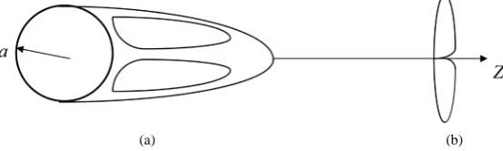
, in the distribution of particle-density flux (4.8). The terms of this order dominate nU at Re1.

Numerical integration of the nonlinear set of 20 algebraic equations was carried out at γ =ˆ 100, and ˆσ =0.5. Calculations have revealed a great many roots. However, at 10<Re≤129.1, the set has only one invariably stable root Сˆi =Сi( )0, i=1,, 20, displayed in Figure 4 in [8]. According to the

(0)

i

С

, i=1,, 20, solution, an axisymmetric recirculating zone is formed in the wake behind the sphere at Re~20. This recirculating zone has the shape of an axisymmetric toroidal ring. It expands as Re grows but its shape remains unchanged (Figure 3(а)). At Re=Re₀*=129.1, the system becomes unstable. At Re1, the Barnett corrections [7] are known to be commensurate with the Navier-Stokes terms. For this reason the calculations [8] were interrupted at

Re 10= .

5. First Unstable Flow Regime

As the flow around sphere becomes unstable, the problem becomes nonstationary. As in the stationary case, the pair distribution function fp

(

t, , ,x G v

)

is represented as

(

)

( )0

₍

₎

₍

₎

, , , , , , ,

p p p

f t x G v = f G v + ∆f t x G v (5.1) Here, f_p( )0

(

G,v

)

is given by Equation (2.2), and ∆f_p

(

t, , ,x G v

)

is given by Equation (2.5) with time-de- pendent coefficients c_klmn. In going to a stationary flow, pair distribution functions lose their main property (17) from [3]. Retaining, as previously, 21 trajectory invariants in expansion (2.5), we arrive at distributions (A.1)-(A.7) from [8] of hydrodynamic values with time-dependent coefficients Cˆ_i=C tˆ_i

( )

, i=1,, 50. Coefficients

( )

ˆ ˆ

i i

C =C t are derived from the condition that hydrodynamic values satisfy boundary conditions (2.14)-(2.16)

(a) (b)

[image:13.595.160.437.614.697.2]