A Hermite Gauss method for the approximation of eigenvalues of regular Sturm Liouville problems

(1)

R E S E A R C H

Open Access

A Hermite-Gauss method for the

approximation of eigenvalues of regular

Sturm-Liouville problems

Rashad M Asharabi

*

*_{Correspondence:}

[email protected] Department of Mathematics, College of Arts and Sciences, Najran University, Najran, Saudi Arabia

Abstract

Recently, some authors have used the sinc-Gaussian sampling technique to approximate eigenvalues of boundary value problems rather than the classical sinc technique because the sinc-Gaussian technique has a convergence rate of the exponential order,O(e–(π–hσ)N/2_/√_N_{), where}

_σ

_,_h_{are positive numbers and}_N_{is the} number of terms in sinc-Gaussian technique. As is well known, the other sampling techniques (classical sinc, generalized sinc, Hermite) have a convergence rate of a polynomial order. In this paper, we use the Hermite-Gauss operator, which is established by Asharabi and Prestin (Numer. Funct. Anal. Optim. 36:419-437, 2015), to construct a new sampling technique to approximate eigenvalues of regular

Sturm-Liouville problems. This technique will be new and its accuracy is higher than the sinc-Gaussian because Hermite-Gauss has a convergence rate of order

O(e–(2π–hσ)N/2_/√_N_{). Numerical examples are given with comparisons with the best} sampling technique up to now,i.e.sinc-Gaussian.

MSC: 34L16; 65L15; 94A20

Keywords: sinc methods; Sturm-Liouville problem; error bounds; convergence rate

1 Introduction

LetEσ(ϕ),σ> , be the class of entire functions satisfying the following condition: _f₍ζ)≤ϕ|ζ|eσ|ζ|, ζ∈C, (.)

where ϕ is a non-decreasing, non-negative function on [,∞). On the class Eσ(ϕ),

Schmeisser and Stenger [] have introduced the so-called sinc-Gaussian operator

Gh,N[f](ζ) :=

n∈ZN(h–ζ)

f(nh)sinch–ζ–ne–Nα(h–ζ–n)_, _(.)

where h∈(,π/σ],α:= (π– hσ)/,N∈N, and

ZN(ζ) :=

n∈Z:[ζ+ /] –n≤N.

(2)

Note that the summation in (.) depends on the real part ofζ. Here, the sinc function is deﬁned as

sinc(t) :=

sin(πt)

πt , t= ,

, t= . (.)

The authors of [] investigated a bound of the approximating function from the classEσ(ϕ)

by the sinc-Gaussian operator. They proved that [], iff∈Eσ(ϕ), then we have forζ∈C, |ζ|<N

f(ζ) –Gh,N[f](ζ)≤sin

h–π ζϕ|ζ|+ h(N+ )EN

h–ζ e –αN

√

π αN, (.)

where

EN(t) :=cosh(αt) +O

N–/, asN→ ∞.

Annaby and Asharabi [] have constructed a new sampling technique to approximate eigenvalues of second order Birkhoﬀ-regular eigenvalue problems using sinc-Gaussian op-erator. Then some authors have used this technique, which is called the sinc-Gaussian technique, to approximate eigenvalues of boundary value problems rather than the clas-sical sinc technique; see, for example, [–]. The convergence rate of sinc-Gaussian tech-nique is of orderO(e–(π–hσ)N/_/√_N_{), where}_σ_,_h_{is deﬁned above, which is highly better}

than the speed of the classical sinc method. The classical sinc method was investigated by Boumenir and Chanane []. Then several studies appeared; seee.g.[, –], with diﬀerent classes of boundary value problems.

For the classEσ(ϕ), Asharabi and Prestin [] deﬁned another localization operatorHh,N,

which is called a Hermite-Gauss operator, as follows:

Hh,N[f](ζ) :=

n∈ZN(h–ζ)

 +β(ζ–nh)



h_N

f(nh) + (ζ–nh)f(nh)

×sinch–ζ–ne–Nβ(h–ζ–n)_, _(.)

whereh∈(, π/σ] andβ:= (π–hσ)/. Forf∈Eσ(ϕ) andζ∈C,|ζ|<Nwe have [] f(ζ) –Hh,N[f](ζ)≤sin

h–π ζϕ|ζ|+h(N+ )EN

h–ζ e –βN

√

πβN, (.)

where

EN(t) :=

eβt/N

√

πβN( – (t/N)₎+

e–βt

( – e–π(N+t)₎+

eβt

( – e–π(N–t)₎

= cosh(βt) +ON–/, asN→ ∞. (.) The bound of (.) shows that the Hermite-Gauss operator has a higher accuracy than the sinc-Gaussian operator because it has a convergence rate of orderO(e–(π–hσ)N/_/√_N_).

(3)

This paper is concerned with constructing a new sampling technique to approximate eigenvalues of Sturm-Liouville problems with separate-type boundary conditions using Hermite-Gauss operatorHh,N. This sampling technique, which is called a Hermite-Gauss

technique, is new and it is expected to give us higher accuracy results. Since alternative samples will be used in our sampling operator, the amplitude error appears in our scheme. For this reason, we will derive estimates for the amplitude error associated with Hermite-Gauss operator,Hh,N. This will be done in the next section. Section  contains the

tech-nique adopted and the associated error analysis. The last section involves numerical ex-amples and comparisons.

2 Amplitude error

In this section, we will investigate the amplitude error associated with the Hermite-Gauss operator (.). The amplitude error arises when the exact valuesf(i)₍_nh_),_i_{= , , of (.)}

are replaced by closer approximate ones. We assume thatf(i)₍_nh_{) are close to}_f(i)₍_nh_),_i.e.

there isε> , suﬃciently small such that

sup

n∈ZN(h–ζ)

f(i)(nh) –f(i)(nh)<ε, (.)

for alli= , . Now, we deﬁne the amplitude error as follows:

AN(ζ) :=Hh,N[f](ζ) –Hh,N[f](ζ)

=

n∈ZN(h–ζ)

f(nh) –f(nh) +β(ζ–nh)



h_N

sinch–ζ–ne–Nβ(h–ζ–n)

+

n∈ZN(h–ζ)

f(nh) –f(nh)(ζ–nh)sinch–ζ–ne–βN(h–ζ–n)_. _(.)

In the following theorem, we will estimate a bound for the amplitude errorAN(z) on

com-plex domainC. Unreservedly, in this paper we need the bound of amplitude error only on a real domain because the eigenvalues of Sturm-Liouville problem (.)-(.) are real numbers but in the general cases the eigenvalues are not necessarily real and this tech-nique will be used for approximating eigenvalues of diﬀerent classes of boundary value problems.

Theorem . Letσ> ,h∈(, π/σ],andβ:= (π–hσ)/.Assume that(.)holds.Then we have forζ∈C,|ζ|<N

AN(ζ)≤ε

 + β

π_N+ h π

( +N/βπ)e(π+βh–)h–|ζ|e–β/N. (.)

Proof From the deﬁnition of the amplitude error (.) and in view of (.), we get

AN(ζ)≤ε

n∈ZN(h–ζ)

_sinc_

h–ζ–n+β|sin

₍_h–_ζ_–_n₎_| π_N

e–Nβ(h–ζ–n)

+εh

π

n∈ZN(h–ζ)

sin

(4)

Sincesincandsinare entire functions of exponential type, we have

sinch–ζ–n≤eh–π|ζ|, sinh–ζ–n≤eh–π|ζ|.

Therefore

AN(ζ)≤ε

 + β

π_N + h π

eh–π|ζ|

n∈ZN(h–ζ)

e–Nβ(h–ζ–n)_. _(.)

Using the inequality

e–ζ_≤_e–(ζ)

e(ζ)

in (.) with the hypothesis|ζ|<Nimplies

_A_N₍ζ)≤ε

 + β

π_N + h π

e(π+βh–)h–|ζ|

n∈ZN(h–ζ)

e–Nβ(h–ζ–n)_. _(.)

The summation in (.) is estimated [], Eq (), as follows:

n∈ZN(h–ζ)

e–Nβ(h–ζ–n)≤_{( +}_N_/_βπ_)e–β/N_. _(.)

Combining (.) and (.) yields (.). In the real domain the bound of the amplitude error will be

A(ε,N) := ε

 + β

π_N + h π

( +N/βπ)e–β/N_, _(.)

which is of the uniform type. This bound will be used when we investigate the error anal-ysis of this technique.

3 The technique and its error analysis

In this section, we discuss the technique and study its error analysis. The error analysis is derived with two types of errors. Now consider the regular Sturm-Liouville problem

–y(t) +q(t)y(t) =μy(t), t∈[,b],μ∈C, (.)

with separate-type boundary conditions

αy(,μ) +αy(,μ) = , (.) αy(b,μ) +αy(b,μ) = , (.)

whereαij∈R, ≤i,j≤ such that|αk|+|αk| = ,k= , , andq(·)∈L[,b] is a real

(5)

conditions:

y(,μ) :=α, y(,μ) := –α. (.)

From the theory of Sturm-Liouville problems,cf. e.g.[, ], the solutiony(x,μ) and its derivativey(x,μ) are entire functions inμfort∈[,b] and problem (.)-(.) has a count-able set of real and simple eigenvalues{μ

j}∞j=owhich can be ordered as an increasing

se-quence tending to inﬁnity,

μ_<μ_<μ_<· · · → ∞.

Moreover, the eigenvalues are the zeros of the characteristic function, which is deﬁned by

D(μ) :=αy(b,μ) +αy(b,μ). (.)

The authors of [] used the successive iterations to prove thatD(·) can be written as

D(μ) = –ααμsin(μb) –ααcos(μb) +αα

∞

n=

Tncos(μb)

–αα

∞

n=

Tnsin(μb)

μ +αα

∞

n=

TTncos(μb)

–αα

∞

n=

TTnsin(μb)

μ , (.)

where the operatorsT andT are Volterra operators acting in the space of continuous functions,C[,b], which are deﬁned, respectively, by

(Ty)(x,μ) :=

x



sinμ(x–t)

μ q(t)y(t,μ)dt, (.)

(Ty)(x,μ) :=

x



cosμ(x–t)q(t)y(t,μ)dt, (.)

andTis the identity operator. All series in (.) converge uniformly on [,b] for any

μ∈C. As i in [] we splitD(·) into parts via

D(μ) =Kk(μ) +Uk(μ), k∈N, (.)

whereKkis known,

Kk(μ) := –ααμsin(bμ) –ααcos(bμ) +αα

k

n=

Tncos(bμ)

–αα

k–

n=

Tnsin(bμ)

μ +αα

k

n=

TTncos(bμ)

–αα

k–

n=

TTnsin(bμ)

(6)

andUk(μ) involves the inﬁnite sum of integral operators

Uk(μ) =αα

∞

n=k+

Tncos(bμ) –αα

∞

n=k

Tnsin(bμ) μ

+αα

∞

n=k+

TTncos(bμ) –αα

∞

n=k

TTnsin(bμ)

μ . (.)

Lemma . Assume that q(·)∈L[,b],then we haveUk(·)∈Eb(ϕ)for all k∈N.

Proof Sinceq(·)∈L_[,_b_{], the solution}_y₍_b_,_μ_{) and its derivative}_y₍_b_,_μ_{) are entire}

func-tions in μ and then D(μ) is an entire function. Therefore, Uk is also an entire

func-tion and then we will prove thatUksatisﬁes the condition (.) of the classEb(ϕ). Since

q(·)∈L[,b], we have,cf. e.g.[], Eq (.)-(.), for allk∈Nandμ∈C

∞

n=k

Tncos(tμ)(b)

≤ρkeb|μ|,

∞

n=k

TTncos(tμ)(b)

≤τρkeb|μ|,

(.) and ∞

n=k

Tn

sin(tμ)

μ

(b)

≤cbρkeb|μ|,

∞

n=k

TTn

_sin

(tμ)

μ

(b)

≤cbτρkeb|μ|,

(.)

whereρk:=∞n=k(cb

τ)n

n! ,τ:= b

|q(t)|dt, andc:= .. Combining (.), (.), and (.),

we obtain for allk∈N

_U_k(μ)≤Mkeb|μ|, (.)

and thusUk(·)∈Eb(ϕ) whereϕ:=Mkis a constant function which is given by

Mk:=|αα|ρk++|αα|cbρk+τ|αα|ρk++cbτ|αα|ρk. (.)

SinceUk(·)∈Eb(ϕ), we approximate the functionUkusing the Hermite-Gauss operator,

(.), whereh∈(, π/b] andβ:= (π–bh)/ and then, from (.), we obtain

_U_k(μ) –Hh,N[Uk](μ)≤TN,h,k(μ), μ∈R, (.)

where the functionTk,h,N is deﬁned as

TN,h,k(μ) := Mksin

h–π μ

 +√ 

πβN

e–βN

√

(7)

In (.), we letμ∈Rbecause all eigenvalues of problem (.)-(.) are real. The samples

Uk(nh) =D(nh) –Kk(nh) andU

k(nh) =D

(nh) –K_k(nh),n∈ZN(h–μ) cannot be computed

explicitly in the general case, so we compute them numerically and this is the reason for the appearance of the amplitude error. According to (.), we have

D(nh) =αy(,nh) +α∂ty(,nh),

D₍_nh_{) =}_α

∂μy(,nh) +α∂μty(,nh).

The solution y(,nh) and its derivative with respect to t, ∂ty(,nh), can be computed

directly by solving the initial value problem deﬁned by (.) and (.) at the nodes

{nh}n∈ZN(h–μ). Also, we can solve the initial value problem (.) and (.) approximately to

ﬁnd the solutiony(,μ) and its derivative,∂ty(,μ), as a function of the parameterμand

consequently, we can easily calculate the derivatives of solution,∂μy(,nh) and∂μty(,nh)

at the nodes{nh}n∈ZN(h–μ). In all examples of Section , we use the code

‘ParametricND-Solve’ ofMathematicato compute these values numerically. Now letUk(nh) andUk(nh)

be the approximations of the samplesUk(nh) andUk(nh),n∈ZN(h–μ), respectively. Let

sup

n∈ZN(h–μ)

_U(i)

k (nh) –U

(i)

k (nh)<ε, i= , .

Therefore we get,cf.Theorem .,

_H_h_,_N[Uk](μ) –Hh,N[Uk](μ)≤A(ε,N), μ∈R, (.)

where A(ε,N) is deﬁned in (.). Now letDN,k(μ) :=Kk(μ) +Hh,N[Uk](μ). Combining

(.), (.), and (.) implies

_D(μ) –DN,k(μ)≤TN,h,k(μ) +A(ε,N), μ∈R. (.)

Now we determine enclosure intervals for the eigenvalues. Let (μ∗)be an eigenvalue, that is, letD(μ∗) = , and (μN,k)be its approximation,i.e.DN.k(μN,k) = . In view of (.), we

obtain

_D_N_,_k

μ∗≤TN,h,k

μ∗+A(ε,N), μ∈R.

SinceDN,k(μ∗) is given andTN,h,k(μ∗) +A(ε,N) is computable, we can deﬁne an enclosure

forμ∗, by solving the following system of inequalities: –TN,h,k

μ∗–A(ε,N)≤DN,k

μ∗≤TN,h,k

μ∗+A(ε,N).

Its solution in an interval will be denoted byIN,k,ε. In the following theorem, we ﬁnd a

bound for the error|μ∗–μN,k|.

Theorem . Let(μ∗)_{be an eigenvalue of problem}_(.)_-_(.)._{For suﬃciently large N}_,_we have the following estimate:

μ∗–μN,k<TN,h,k

(μN,k) +A(ε,N)

infζ∈IN,k,ε|D(ζ)|

, (.)

(8)

Proof SinceD(μN,k) –DN.k(μN,k) =D(μN,k) –D(μ∗), then from (.) and after replacing

μbyμN,kwe get

_D(μN,k) –D

μ∗≤TN,h,k(μN,k) +A(ε,N).

Using the mean value theorem yields

μ∗–μN,k

D₍_ζ₎_≤_T

N,h,k(μN,k) +A(ε,N), ζ∈JN,k⊂IN,k,ε, (.)

for someζ∈JN,k:= (min{μ∗,μN,k},max{μ∗,μN,k}). Since the zeros ofD(μ) are simple, for

suﬃciently largeNwe haveinfζ∈IN,k,ε|D

₍_ζ₎_|_{>  and then we get (.). In view of (.)}

and (.), the right hand-side of (.) goes to zero uniformly whenN→ ∞andε→, and therefore|μ∗–μN,k| → for allk∈N.

4 Examples and comparisons

This section includes three examples to illustrate our technique. All examples are com-puted in [] with the Hermite sampling technique and the authors compare their results with the results of the classical sinc technique. In our approximations,Kk of (.) has

fewer terms than is used in []. Note that the accuracy of any sampling technique increases whenN is ﬁxed butkincreases. As is well known, the sinc-Gaussian is better than the other sampling techniques (classical sinc, generalized sinc, Hermite) because of the con-vergence rate of all these techniques being of polynomial order; seee.g.[, , , –]. As we mentioned before, the sinc-Gaussian has convergence rate of an exponential order. Therefore, we compare our results only with the results of the sinc-Gaussian technique. As predicted by the error estimates, the Hermite-Gauss technique gives us a higher accuracy result than the results of sinc-Gaussian technique and the accuracy increases whenNis ﬁxed, buthdecreases without any additional cost except that the function is approximated on a smaller domain. Denote byEGandEHthe absolute errors associated with the results

of the sinc-Gaussian and Hermite-Gauss technique, respectively. We useMathematicato derive the following examples.

Example . Consider the Sturm-Liouville problem

–y(t) –y(t) =μy(t), t∈[, ], (.) with the separate boundary condition of the form

y(,μ) =y(,μ) = . (.) In this case, the characteristic function is

D(μ) :=cos +μ_, _(.)

and the exact eigenvalues are μ_l := (l+ )π/ – ,l∈Z. Takingk=  in (.) and making some computations gives

K(μ) =cos(μ) – sin(μ)

μ +

(9)

[image:9.595.158.437.97.165.2]

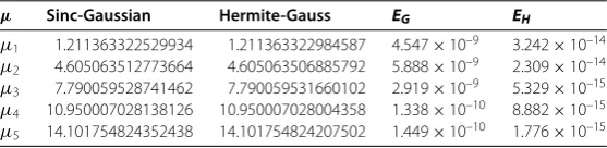
Table 1 Comparison of Hermite-Gauss and sinc-Gaussian,N= 7 andh= 1

μ Sinc-Gaussian Hermite-Gauss EG EH

[image:9.595.159.438.199.265.2]

μ1 1.211363322529934 1.211363322984587 4.547×10–9 3.242×10–14 μ2 4.605063512773664 4.605063506885792 5.888×10–9 2.309×10–14 μ3 7.790059528741462 7.790059531660102 2.919×10–9 5.329×10–15 μ4 10.950007028138126 10.950007028004358 1.338×10–10 8.882×10–15 μ5 14.101754824352438 14.101754824207502 1.449×10–10 1.776×10–15

μ1 2.978188104491012 2.978188107069353 2.578×10–9 3.553×10–14 μ2 6.203097476060051 6.203097420189766 5.587×10–8 6.048×10–13 μ3 9.371576077716716 9.371576153977529 7.626×10–8 2.114×10–13 μ4 12.526518591941482 12.526518687065739 9.513×10–8 9.006×10–13 μ5 15.676099922268510 15.676099962274689 4.001×10–8 1.741×10–13

and thenU∈B∞ . Table  shows the ﬁrst ﬁve approximate eigenvalues of problem

(.)-(.) using our techniques withN=  andh=  comparing with the results of the sinc-Gaussian technique.

Example . The boundary value problem

–y(t) –y(t) =μy(t), t∈[, ], (.)

y(,μ) =y(,μ) = , (.) is a special case of problem (.)-(.) whenα=α=  andα=α= . The

character-istic function of this problem is

D(μ) := –sin(

 +μ₎

 +μ , (.)

and the exact eigenvalues areμ

l := (πl)– ,l∈Z. Takingk=  in (.), we have after

some calculations

K(μ) = – sinμ

μ +

sin(μ) –μcos(μ) μ .

Table  lists the ﬁrst ﬁve approximate eigenvalues using our technique withN=  and

h=  in comparison with the results of the sinc-Gaussian technique.

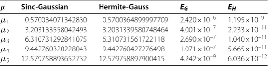
Example . In this example, we introduce the Sturm-Liouville problem

–y(t) +ty(t) =μy(t), t∈[, ], (.)

y(,μ) =y(,μ) = . (.) The characteristic function is

D(μ) := –F

 

 –μ, ; 

+ –μF

 + 

 –μ, ; 

(10)

[image:10.595.160.435.97.165.2]

μ1 0.570034071342830 0.5700364899997709 2.420×10–6 1.195×10–9 μ2 3.203133558042493 3.2031339580748464 4.001×10–7 2.233×10–11 μ3 6.310731292841075 6.310731561722118 2.690×10–7 1.040×10–11 μ4 9.442760320228043 9.442760427276498 1.071×10–7 5.665×10–11 μ5 12.579758893652732 12.579758897900415 4.242×10–9 6.036×10–12

whereFis the hypergeometric function. In this case, puttingk=  in (.) implies after some calculations

K(μ) := –μsin(μ) +

μ( + μ₎_cos_μ_{+ (}_μ_{– )}_sin_μ

μ .

As in the last examples, we summarize our results of this example in Table . To compute the absolute error, the exact eigenvalues are computed approximately byMathematica.

Competing interests

The author declares that he has no competing interests.

Acknowledgements

The author would like to thank the anonymous referees for their constructive comments.

Received: 26 February 2016 Accepted: 1 June 2016 References

1. Asharabi, RM, Prestin, J: A modiﬁcation of Hermite sampling with a Gaussian multiplier. Numer. Funct. Anal. Optim. 36, 419-437 (2015)

2. Schmeisser, G, Stenger, F: Sinc approximation with a Gaussian multiplier. Sampl. Theory Signal Image Process., Int. J. 6, 199-221 (2007)

3. Annaby, MH, Asharabi, RM: Computing eigenvalues of boundary-value problems using sinc-Gaussian method. Sampl. Theory Signal Image Process., Int. J.7, 293-311 (2008)

4. Annaby, MH, Tharwat, MM: A sinc-Gaussian technique for computing eigenvalues of second-order linear pencils. Appl. Numer. Math.63, 129-137 (2013)

5. Tharwat, MM, Al-Harbi, SM: Approximation of eigenvalues of boundary value problems. Bound. Value Probl. (2014). doi:10.1186/1687-2770-2014-51

6. Tharwat, MM, Bhrawy, AH, Aloﬁ, AS: Approximation of eigenvalues of discontinuous Sturm-Liouville problems with eigenparameter in all boundary conditions. Bound. Value Probl. (2013). doi:10.1186/1687-2770-2013-132 7. Boumenir, A, Chanane, B: Eigenvalues of Sturm-Liouville systems using sampling theory. Appl. Anal.62, 323-334

(1996)

8. Annaby, MH, Asharabi, RM: On sinc-based method in computing eigenvalues of boundary-value problems. SIAM J. Numer. Anal.46(2), 671-690 (2008)

9. Annaby, MH, Asharabi, RM: Approximating eigenvalues of discontinuous problems by sampling theorems. J. Numer. Math.3, 163-183 (2008)

10. Annaby, MH, Tharwat, MM: On computing eigenvalues of second-order linear pencils. IMA J. Numer. Anal.27, 366-380 (2007)

11. Asharabi, RM: Generalized sinc-Gaussian sampling involving derivatives. Numer. Algorithms (2016). doi:10.1007/s11075-016-0129-4

12. Asharabi, RM, Prestin, J: On two-dimensional classical and Hermite sampling. IMA J. Numer. Anal.36, 851-871 (2016) 13. Levitan, BM, Sargsjan, IS: Introduction to Spectral Theory: Selfadjoint Ordinary Diﬀerential Operators. Translation of

Mathematical Monographs, vol. 39. Am. Math. Soc., Providence (1975)

14. Titchmarch, EC: Eigenfunction Expansions Associated with Second-Order Diﬀerential Equations, 2nd edn. Clarendon Press, Oxford (1962)

15. Annaby, MH, Asharabi, RM: Computing eigenvalues of Sturm-Liouville problems by Hermite interpolations. Numer. Algorithms60, 355-367 (2012)

16. Boumenir, A: The sampling method for Sturm-Liouville problems with the eigenvalue parameter in the boundary condition. Numer. Funct. Anal. Optim.21, 67-75 (2000)