Approximation of eigenvalues of discontinuous Sturm-Liouville problems with eigenparameter in all boundary conditions

R E S E A R C H

Open Access

Approximation of eigenvalues of

discontinuous Sturm-Liouville problems with

eigenparameter in all boundary conditions

Mohammed M Tharwat

_{, Ali H Bhrawy}

_{and Abdulaziz S Alofi}

*_{Correspondence:}

[email protected]

1_{Department of Mathematics,}

Faculty of Science, King Abdulaziz University, Jeddah, Saudi Arabia

2_{Permanent address: Department of}

Mathematics, Faculty of Science, Beni-Suef University, Beni-Suef, Egypt

Abstract

In this paper, we apply a sinc-Gaussian technique to compute approximate values of the eigenvalues of Sturm-Liouville problems which contain an eigenparameter appearing linearly in two boundary conditions, in addition to an internal point of discontinuity. The error of this method decays exponentially in terms of the number of involved samples. Therefore the accuracy of the new technique is higher than that of the classical sinc method. Numerical worked examples with tables and illustrative figures are given at the end of the paper.

MSC: 34L16; 94A20; 65L15

Keywords: sampling theory; Sturm-Liouville problems; transmission conditions; sinc-Gaussian; sinc method; truncation and amplitude errors

1 Introduction

By a sampling theorem we mean a representation of a certain function in terms of its values at a discrete set of points. In communication theory, it means a reconstruction of a signal (information) in terms of a discrete set of data. This has several applications, especially in the transmission of information. If the signal is band-limited, the sampling process can be done via the celebrated Whittaker-Kotel’nikov-Shannon (WKS) sampling theorem [–]. By a band-limited signal with band widthτ,τ> , we mean a function in the Paley-Wiener space

Bτ :=

f entire,f(λ)≤Ceτ|λ|,

R

_f(λ)dλ

. (.)

The WKS sampling theorem is a fundamental result in information theory. It states that anyf∈Bτ can be reconstructed from its sampled valuesf(xk), wherexk=kπ/τandk∈Z,

by the formula

f(x) =

k∈Z

f(xk)sinc(τx/π–k), x∈R, (.)

where

sinc(x) :=

⎧ ⎨ ⎩

sinπx

πx , x∈R\ {},

, x= , (.)

and the series converges absolutely and uniformly on any finite interval ofR. Expansion (.) is used in several approximation problems which are known as sinc methods; see,e.g., [–]. In particular the sinc-method is used to approximate eigenvalues of boundary value problems; see, for example, [–]. The sinc-method has a slow rate of decay at infinity, which is as slow asO(|x–_{|). There are several attempts to improve the rate of decay. One} of the interesting ways is to multiply the sinc-function in (.) by a kernel function; see, e.g., [–]. Leth∈(,π/τ] andγ ∈(,π–hτ). Assume that∈Bγ such that() = ,

then forf∈Bτ we have the expansion, []

f(x) = ∞

n=–∞

f(nh)sinch–πx–nπh–x–n. (.)

The speed of convergence of the series in (.) is determined by the decay of|(x)|. But the decay of an entire function of exponential type cannot be as fast ase–c|x|_{as|x| −→ ∞,}

for some positivec[]. In [], Qian has introduced the following regularized sampling formula. Forh∈(,π/τ],N∈Nandr> , Qian defined the operator []

(Gh,Nf)(x) =

n∈ZN(x)

f(nh)Sn

h–πxG

x–nh √

rh

, x∈R, (.)

whereG(t) :=exp(–t_{), which is called the Gaussian function,S}

n(h–πx) :=sinc(h–πx–

nπ),ZN(x) :={n∈Z:|[h–x] –n| ≤N}and [x] denotes the integer part ofx∈R; see also

[, ]. Qian also derived the following error bound. If f ∈Bτ,h∈(,π/τ] anda:=

min{r(π–hτ), (N– )/r} ≥, then [, ]

f(x) – (Gh,Nf)(x)≤

√τ π f 

π_a

√

πa+e/re–a/, x∈R. (.)

In [] Schmeisser and Stenger extended the operator (.) to the complex domainC. For

τ > ,h∈(,π/τ] andω:= (π–hτ)/, they defined the operator []

(Gh,Nf)(z) :=

n∈ZN(z)

f(nh)Sn

πz h

G

√

ω(z–nh) √

Nh

, (.)

where ZN(z) :={n∈Z:|[h–_{z+ /] –n| ≤N} andN∈N. Note that the summation} limits in (.) depend on the real part ofz. Schmeisser and Stenger [] proved that iff is an entire function such that

f(ξ+iη)≤φ|ξ|eτ|η|_{, ξ,η∈R, (.)}

where φ is a non-decreasing, non-negative function on [,∞) andτ ≥, then forh∈ (,π/τ),ω:= (π–hτ)/,N∈N,|z|<N, we have

_{f(z) – (Gh,Nf)(z)}

≤sinh–πzφ|z|+h(N+ ) e –ωN

√

π ωNβN

where

βN(t) :=cosh(ωt) +

eωt/N

√

π ωN[ – (t/N)_]+  

eωt

eπ(N–t)_{– }+ e–ωt

eπ(N+t)_{– }

. (.)

The amplitude error arises when the exact valuesf(nh) of (.) are replaced by the ap-proximationsf(nh). We assume thatf(nh) are close tof(nh),i.e., there isε>  sufficiently small such that

sup n∈Zn(z)

f(nh) –f(nh)<ε. (.)

Leth∈(,π/τ),ω:= (π–hτ)/ andN∈Nbe fixed numbers. The authors in [] proved that if (.) holds, then for|z|<N, we have

(Gh,Nf)(z) – (Gh,Nf)(z)≤Aε,N(z), (.)

where

Aε,N(z) = εe–ω/N( +

√

N/ωπ)exp(ω+π)h–|z|. (.) It is well known that many topics in mathematical physics require the investigation of the eigenvalues and eigenfunctions of Sturm-Liouville type boundary value problems. There-fore, the Sturmian theory is one of the most actual and extensively developing fields of theoretical and applied mathematics. Particularly, in recent years, highly important re-sults in this field have been obtained for the case when the eigenparameter appears not only in the differential equation but also in the boundary conditions. The literature on such results is voluminous, and we refer to [–] and corresponding bibliography cited therein. In particular, [, , , ] contain many references to problems in physics and mechanics. Our task is to use formula (.) to compute the eigenvalues numerically of the differential equation

–y(x,μ) +q(x)y(x,μ) =μy(x,μ), x∈–, )∪(, , (.)

with boundary conditions

L(y) :=

α_μ–α

y(–,μ) –α_μ–α

y(–,μ) = , (.)

L(y) :=

β_μ+β

y(,μ) –β_μ+β

y(,μ) = , (.)

and transmission conditions

L(y) :=γy

–,μ–δy

+,μ= , (.)

L(y) :=γy

–,μ–δy

+,μ= , (.)

β_i(i= , ) are real numbers;γi= ,δi=  (i = , );γγ=δδand

det

α_ α

α_ α

> , det

β_ β

β_ β

> . (.)

The eigenvalue problem (.)-(.) when (α_,α_)= (, ) = (β_,β_) is a Sturm-Liouville problem which contains an eigenparameterμin two boundary conditions, in addition to an internal point of discontinuity. In [], Tharwat proved that the eigenvalue prob-lem (.)-(.) has a denumerable set of real and simple eigenvalues using techniques similar to those established in [, , ], where also sampling theorems have been es-tablished. Tharwatet al., in [], computed the eigenvalues of the problem (.)-(.) by using the sinc method. In the sinc method, the basic idea is as follows: The eigenvalues are characterized as the zeros of an analytic functionF(μ) which can be written in the formF(μ) =K(μ) +U(μ), whereK(μ) (known part) is the function for the caseq≡. The ingenuity of the approach is in trying to choose the functionF(μ) so thatU(μ)∈Bτ

(unknown part) and can be approximated by the WKS sampling theorem if its values at some equally spaced points are known; see [–].

Our goal in this paper is to improve the results presented in Tharwatet al.[] with the least conditions. In this paper we use the sinc-Gaussian sampling formula (.) to compute eigenvalues of (.)-(.) numerically. As is expected, the new method reduced the error bounds remarkably; see the examples at the end of this paper. Also here, we use the same idea but the unknown partU(μ) is an entire function of exponential type and satisfies (.), that is,U(μ) is not necessaryL-function. Then we approximate theU(μ) using (.) and obtain better results. We would like to mention that the papers in computing eigenvalues by the Gaussian method are few; see [, , ]. In Section  we derive the sinc-Gaussian technique to compute the eigenvalues of (.)-(.) with error estimates. The last section involves some illustrative examples.

2 Treatment of the eigenvalue problem (1.14)-(1.18)

In this section we derive approximate values of the eigenvalues of the eigenvalue problem (.)-(.). Recall that the problem (.)-(.) has a denumerable set of real and simple eigenvalues,cf.[]. Let

y(x,μ) =

⎧ ⎨ ⎩

y(x,μ), x∈[–, ),

y(x,μ), x∈(, ]

denote the solution of (.) satisfying the following initial conditions:

y(–,μ) y(+,μ)

y_(–,μ) y_(+,μ)

=

μα_–α γδy( –_,μ)

μα_–α γδy

(–,μ)

. (.)

Sincey(·,μ) satisfies (.), (.) and (.), then the eigenvalues of problem (.)-(.) are the zeros of the characteristic determinant,cf.[],

(μ) :=β_μ+β

y(,μ) –

β_μ+β

According to [], see also [–], the function(μ) is an entire function ofμwhere zeros are real and simple. We aim to approximate(μ) and hence its zeros,i.e., the eigen-values, by using (.). The idea is to split(μ) into two parts, one is known and the other is unknown, but is an entire function of exponential type and satisfies (.). Then we ap-proximate the unknown part using (.) to get the apap-proximate(μ) and then compute the approximate zeros. By using the method of variation of constants, we can see that the solutiony(·,μ) satisfies the Volterra integral equations,cf.[],

y(x,μ) =

–α+μα

cosμ(x+ )––α+μα



μsin

μ(x+ )

+ (Ty)(x,μ), (.)

y(x,μ) =

γ

δ

y

–,μcos[μx] +γ

δ

y_–,μsin[μx]

μ + (Ty)(x,μ), (.)

whereTandTare the Volterra operators

(Ty)(x,μ) :=

x

–

sin[μ(x–t)]

μ q(t)y(t,μ)dt, (.)

(Ty)(x,μ) :=

x



sin[μ(x–t)]

μ q(t)y(t,μ)dt. (.)

Differentiating (.) and (.), we obtain

y_(x,μ) = ––α+μα

μsinμ(x+ )––α+μα

cosμ(x+ )

+ (Ty)(x,μ), (.)

y_(x,μ) = –γ

δ

μy

–,μsin[μx] +γ

δ

y_–,μcos[μx] + (Ty)(x,μ), (.)

whereTandTare the Volterra-type integral operators

(Ty)(x,μ) :=

x

–

cosμ(x–t)q(t)y(t,μ)dt, (.)

(Ty)(x,μ) :=

x



cosμ(x–t)q(t)y(t,μ)dt. (.)

Defineϑi(·,μ) andϑi(·,μ),i= , , to be

ϑi(x,μ) :=Tiyi(x,μ), ϑ˜i(x,μ) :=Tiyi(x,μ). (.)

In the following, we make use of the known estimates []

|cosz| ≤e|z|, sinz z

≤ c

 +|z|e

wherecis some constant (we may takec.cf.[]). For convenience, we define the constants

q:=

 –

q(t)dt, q:=

 

q(t)dt, c:=max

|α|,|α|,|α|,|α|

,

c:=exp(cq), c:=  +ccq,

c:= ( +c)

_|

γ| |δ|

c+|

γ| |δ|

c( +cq)

,

c:=exp(cq), c:=  +cqc.

(.)

As in [], we split(μ) into two parts via

(μ) :=K(μ) +U(μ), (.)

whereK(μ) is the known part

K(μ) :=β_μ+β

μα_–α

γ

δ

cosμ–γ

δ sinμ

–μα_–α

γ

δ +γ

δ

cosμsinμ μ

+β_μ+β

μα_–α

γ

δ +γ

δ

μcosμsinμ

+μα_–α

γ

δ

cosμ–γ

δ sinμ

(.)

andU(μ) is the unknown one

U(μ) := γ

δ

β_μ+β

cosμ+β_μ+β

μsinμϑ

–,μ+β_μ+β

ϑ(,μ)

+γ

δ

β_μ+β

sinμ

μ –

β_μ+β

cosμ

ϑ

–,μ

–β_μ+βϑ(,μ). (.)

Then the functionU(μ) is entire inμfor eachx∈[, ] for which,cf.[],

_U(μ)≤φ|μ|e|μ|_{, μ∈C, (.)}

where

φ|μ|:=M +|μ|, (.)

and

M:=cc( +c)q

cc|

γ| |δ|

+c|

γ| |δ|

+cccq(c+cc),

c:=max|β|,|β|,β,β.

(.)

since all eigenvalues are real. Now we approximate the functionU(μ) using the operator (.) whereh∈(,π/) andω:= (π– h)/ and then, from (.), we obtain

_U(μ) – (Gh,NU)(μ)≤Th,N(μ), (.)

where

Th,N(μ) := sin

h–π μφ|μ|+h(N+ ) e –ωN

√

π ωNβN(), μ∈R. (.)

The samplesU(nh) =(nh) –K(nh),n∈ZN(μ) cannot be computed explicitly in the gen-eral case. We approximate these samples numerically by solving the initial-value prob-lems defined by (.) and (.) to obtain the approximate valuesU(nh),n∈ZN(μ),i.e.,

U(nh) =(nh) –K(nh). Here we use a computer algebra system, Mathematica, to ob-tain the approximate solutions with the required accuracy. However, a separate study for the effect of different numerical schemes and the computational costs would be interest-ing. Accordingly, we have the explicit expansion

(Gh,NU)(μ) :=

n∈ZN(μ)

U(nh)Sn

π μ

h

G

√

ω(μ–nh) √

Nh

. (.)

Therefore we get,cf.(.),

(Gh,NU)(μ) – (Gh,NU)(μ)≤Aε,N(), μ∈R. (.)

Now letN(μ) :=K(μ) + (Gh,NU)(μ). From (.) and (.) we obtain

(μ) –N(μ)≤Th,N(μ) +Aε,N(), μ∈R. (.)

Let μ∗ be an eigenvalue and μN be its desired approximation, i.e., (μ∗) =  and

N(μN) = . From (.) we have|N(μ∗)| ≤Th,N(μ∗) +Aε,N(). Define the curves

a±(μ) =N(μ)±Th,N(μ) +Aε,N(). (.)

The curvesa+(μ),a–(μ) trap the curve of(μ) for suitably largeN. Hence the closure interval is determined by solvinga±(μ) = , which gives an interval

Iε,N := [a–,a+].

It is worthwhile to mention that the simplicity of the eigenvalues guarantees the existence of approximate eigenvalues, i.e., theμN’s for which N(μN) = . Next we estimate the

error|μ∗–μN|for the eigenvalueμ∗.

Theorem . Letμ∗be an eigenvalue of(.)-(.)andμN be its approximation.Then,

forμ∈R,we have the following estimate:

μ∗–μN<

Th,N(μN) +Aε,N() inf

ζ∈Iε,N|

(ζ)| , (.)

Proof ReplacingμbyμN in (.), we obtain

(μN) –

μ∗<Th,N(μN) +Aε,N(), (.)

where we have usedN(μN) =(μ∗) = . Using the mean value theorem yields that for someζ ∈Jε,N:= [min(μ∗,μN),max(μ∗,μN)],

μ∗–μN

(ζ)≤Th,N(μN) +Aε,N(), ζ∈Jε,N⊂Iε,N. (.)

Sinceμ∗is simple andNis sufficiently large, theninfζ∈Iε,N|(ζ)|> , and we get (.).

3 Examples

This section includes two examples illustrating the sinc-Gaussian method. All exam-ples are computed in [] with the classical method. It is clearly seen that the sinc-Gaussian method gives remarkably better results. We indicate in these two examples the effect of the amplitude error in the method by determining enclosure intervals for differ-ent values ofε. We also indicate the effect ofNandhby several choices. We would like to mention that Mathematica has been used to obtain the exact values for these examples where eigenvalues cannot computed concretely. Mathematica is also used in rounding the exact eigenvalues, which are square roots. Each example is exhibited via figures that accurately illustrate the procedure near to some of the approximated eigenvalues. More explanations are given below.

Example  Consider the boundary value problem

–y(x,μ) +q(x)y(x,μ) =μy(x,μ), x∈[–, )∪(, ], (.)

μy(–,μ) +y(–,μ) = , μy(,μ) –y(,μ) = , (.)

y–,μ–y+,μ= , y–,μ–y+,μ= . (.) Hereβ_=β=α=α= ,β=β=α=α= ,γ=δ= ,γ=δ=_ and

q(x) =

⎧ ⎨ ⎩

–, x∈[–, ),

–, x∈(, ]. (.)

The characteristic function is

(μ) = 

 +μ_{ +μ}

sin +μ_{– +μ}_μ_–μ_{– cos +μ} –μ + μsin +μ

– +μ_{cos +μ}_–μ_{ +μ}_{cos +μ}

+μ–μ– sin +μ_{. (.)} The functionK(μ) will be

Table 1 The approximationμk,Nand the exact solutionμkfor different choices ofhandN

μk

μ1 μ2 μ3 μ4

Exactμk 0.579603114810978 1.7849838948888357 3.238647349751419 4.770562335590527

μk,N h= 0.5,

ω= 1.0708

N= 10 0.5795964187714981 1.7849867099956038 3.2386476744424746 4.770562422264749

N= 20 0.5796031144857375 1.7849838950724857 3.2386473497857042 4.770562335603019

h= 0.1, ω= 1.4708

N= 10 0.5796031130499404 1.7849838962430518 3.2386473440949666 4.770562334447039

N= 20 0.579603114810984 1.7849838948888386 3.2386473497514174 4.770562335590528

Table 2 Absolute error|μ_k–μ_k,N|

μk

μ1 μ2 μ3 μ4

h= 0.5 N= 10 6.69604×10–6 2.81511×10–6 3.24691×10–7 8.66742×10–8

N= 20 3.25241_×10–10 _1.8365×10–10 _3.4285×10–11 _1.24922×10–11 h= 0.1 N= 10 1.76104_×10–9 _1.35422×10–9 _5.65645×10–9 _1.14349×10–9

N= 20 5.9952×10–15 _2.88658×10–15 _1.77636×10–15 _8.88178×10–16

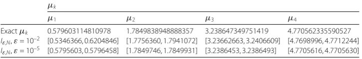
Table 3 ForN= 20 andh= 0.1, the exact solutionsμkare all inside the interval [a–,a+] for

different values ofε

μk

μ1 μ2 μ3 μ4

Exactμk 0.579603114810978 1.7849838948888357 3.238647349751419 4.770562335590527 Iε,N,ε= 10–2 [0.5346366, 0.6204846] [1.7756360, 1.7941072] [3.23662663, 3.2406609] [4.7698996, 4.7712244] Iε,N,ε= 10–5 [0.5795603, 0.5796458] [1.7849746, 1.7849931] [3.2386453, 3.2386493] [4.7705616, 4.7705630]

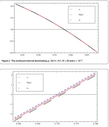
Figure 2 The enclosure interval dominatingμ1forh= 0.1,N= 20 andε= 10–5.

Figure 3 The enclosure interval dominatingμ4forh= 0.1,N= 20 andε= 10–2.

As is clearly seen, eigenvalues cannot be computed explicitly. Tables , ,  indicate the application of our technique to this problem and the effect ofε. By exact we mean the zeros of(μ) computed by Mathematica.

Figures  and  illustrate the enclosure intervals dominatingμforN= ,h= . and

ε= –_{,ε= }–_{, respectively. The middle curve represents(μ), while the upper and} lower curves represent the curves ofa+(μ),a–(μ), respectively. We notice that whenε= –, all two curves are almost identical. Similarly, Figures  and  illustrate the enclosure intervals dominatingμforh= .,N=  andε= –,ε= –, respectively.

Example  Consider the boundary value problem

–y(x,μ) +q(x)y(x,μ) =μy(x,μ), x∈[–, )∪(, ], (.)

y(–,μ) +μy(–,μ) = , y(,μ) +μy(,μ) = , (.)

Figure 4 The enclosure interval dominatingμ4forh= 0.1,N= 20 andε= 10–5.

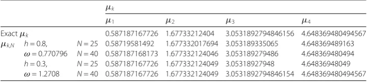
Table 4 The approximationμ_k,Nand the exact solutionμ_kfor different choices ofhandN

μk

μ1 μ2 μ3 μ4

Exactμk 0.587187167726 1.67733212404 3.0531892794846156 4.648369480494567

μk,N h= 0.8,

ω= 0.770796

N= 25 0.58719581492 1.677332017694 3.053189335065 4.648369489163

N= 40 0.587187168173 1.677332124046 3.053189279486 4.648369480494

h= 0.3, ω= 1.2708

N= 25 0.587187167726 1.677332124049 3.05318927948 4.64836948049

N= 40 0.587187167726 1.677332124049 3.0531892794846154 4.648369480494567

Table 5 Absolute error|μk–μk,N|

μk

μ1 μ2 μ3 μ4

h= 0.8 N= 25 8.6472×10–6 _1.06355×10–7 _5.55809×10–8 _8.66884×10–9 N= 40 4.47627×10–10 _2.99827×10–12 _2.33413×10–12 _3.41061×10–13 h= 0.3 N= 25 1.12133×10–13 _6.83897×10–14 _3.55271×10–15 _4.440895×10–15

N= 40 5.55112×10–16 _2.22045×10–16 _1.965×10–16 _5.56×10–16

Table 6 ForN= 40 andh= 0.3, the exact solutionsμ_kare all inside the interval [a–,a+] for

different values ofε

μk

μ1 μ2 μ3 μ4

Exactμk 0.5871871677260395 1.677332124049779 3.05318927948461569256 4.6483694804945678959

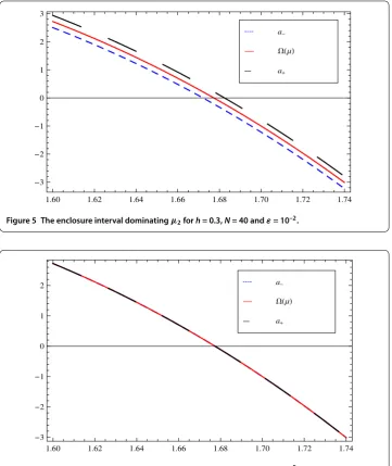
Figure 5 The enclosure interval dominatingμ2forh= 0.3,N= 40 andε= 10–2.

Figure 6 The enclosure interval dominatingμ2forh= 0.3,N= 40 andε= 10–5.

whereα=β= ,α=β= –,β=β=α=α= ,γ=δ= ,γ=δ=_ and

q(x) =

⎧ ⎨ ⎩

–, x∈[–, ),

x, x∈(, ]. (.)

The function K(μ) will be

K(μ) =( +μ _)sinμ

μ . (.)

The characteristic determinant of the problem is

(μ) = – π  +μ

–Bi –μ+μBi –μ

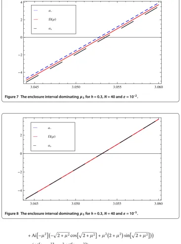
Figure 7 The enclosure interval dominatingμ3forh= 0.3,N= 40 andε= 10–2.

Figure 8 The enclosure interval dominatingμ3forh= 0.3,N= 40 andε= 10–5.

+Ai–μ– +μ_{cos +μ}_+μ_{ +μ}_{sin +μ} +Ai –μ+μAi –μ

×Bi–μμ +μ_{cos +μ}_{+sin +μ}

+Bi–μ– +μ_{cos +μ}_+μ_{ +μ}_{sin +μ}_{, (.)}

whereAi[z] andBi[z] are Airy functions, andAi[z] andBi[z] are derivatives of Airy func-tions. As in the above example, the three tables (Tables , , ) indicate the application of our technique to this problem and the effect ofε.

4 Conclusion

With a simple analysis, and with values of solutions of initial value problems computed at a few values of the eigenparameter, we have computed the eigenvalues of discontinu-ous Sturm-Liouville problems which contain an eigenparameter appearing linearly in two boundary conditions, with a certain estimated error. The method proposed is a shooting procedure,i.e., the problem is reformulated as two initial value ones, due to the interior discontinuity, of size two and a miss-distance is defined at the right end of the interval of integration whose roots are the eigenvalues to be computed. The unknown partU(μ) of the miss-distance can be written in terms of a function which is an entire function of ex-ponential type. Therefore, we propose to approximate such term by means of a truncated cardinal series with sampling values approximated by solving numerically corresponding suitable initial value problems. Finally, in Section  we introduced two instructive exam-ples. The computations show that, as compared to the classical sampling expansion in [], the variant with the Gaussian multiplier provides a strikingly high improvement of the accuracy.

Competing interests

The authors declare that they have no competing interests.

Authors’ contributions

The authors have equal contributions to each part of this article. All the authors read and approved the final manuscript.

Acknowledgements

This work was funded by the Deanship of Scientific Research (DSR), King Abdulaziz University, Jeddah, under grant No. (130-065-D1433). The authors, therefore, acknowledge with thanks DSR technical and financial support.

Received: 12 March 2013 Accepted: 4 May 2013 Published: 20 May 2013

References

1. Kotel’nikov, V: On the carrying capacity of the ‘ether’ and wire in telecommunications. In: Material for the First All-Union Conference on Questions of Communications, vol. 55, pp. 55-64. Izd. Red. Upr. Svyazi RKKA, Moscow (1933) 2. Shannon, CE: Communications in the presence of noise. Proc. IRE37, 10-21 (1949)

3. Whittaker, ET: On the functions which are represented by the expansion of the interpolation theory. Proc. R. Soc. Edinb., Sect. A35, 181-194 (1915)

4. Stenger, F: Numerical methods based on Whittaker cardinal, or sinc functions. SIAM Rev.23, 156-224 (1981) 5. Lund, J, Bowers, K: Sinc Methods for Quadrature and Differential Equations. SIAM, Philadelphia (1992) 6. Stenger, F: Numerical Methods Based on Sinc and Analytic Functions. Springer, New York (1993)

7. Kowalski, M, Sikorski, K, Stenger, F: Selected Topics in Approximation and Computation. Oxford University Press, New York (1995)

8. Boumenir, A: Higher approximation of eigenvalues by sampling. BIT Numer. Math.40, 215-225 (2000) 9. Boumenir, A: Sampling and eigenvalues of non-self-adjoint Sturm-Liouville problems. SIAM J. Sci. Comput.23,

219-229 (2001)

10. Annaby, MH, Tharwat, MM: On computing eigenvalues of second-order linear pencils. IMA J. Numer. Anal.27, 366-380 (2007)

11. Annaby, MH, Tharwat, MM: Sinc-based computations of eigenvalues of Dirac systems. BIT Numer. Math.47, 699-713 (2007)

12. Annaby, MH, Tharwat, MM: On the computation of the eigenvalues of Dirac systems. Calcolo49, 221-240 (2012) 13. Tharwat, MM, Bhrawy, AH, Yildirim, A: Numerical computation of eigenvalues of discontinuous Dirac system using

Sinc method with error analysis. Int. J. Comput. Math.89, 2061-2080 (2012)

14. Tharwat, MM, Bhrawy, AH, Yildirim, A: Numerical computation of eigenvalues of discontinuous Sturm-Liouville problems with parameter dependent boundary conditions using Sinc method. Numer. Algorithms63, 27-48 (2013) 15. Gervais, R, Rahman, QI, Schmeisser, G: A bandlimited function simulating a duration-limited one. In: Butzer, PL, Stens,

RL (eds.) Approximation Theory and Functional Analysis, pp. 355-362. Birkhäuser, Basel (1984)

16. Butzer, PL, Stens, RL: A modification of the Whittaker-Kotel’nikov-Shannon sampling series. Aequ. Math.28, 305-311 (1985)

17. Stens, RL: Sampling by generalized kernels. In: Higgins, JR, Stens, RL (eds.) Sampling Theory in Fourier and Signal Analysis: Advanced Topics, pp. 130-157. Oxford University Press, Oxford (1999)

18. Schmeisser, G, Stenger, F: Sinc approximation with a Gaussian multiplier. Sampl. Theory Signal. Image Process, Int. J. 6, 199-221 (2007)

19. Qian, L: On the regularized Whittaker-Kotel’nikov-Shannon sampling formula. Proc. Am. Math. Soc.131, 1169-1176 (2002)

21. Qian, L, Creamer, DB: Localized sampling in the presence of noise. Appl. Math. Lett.19, 351-355 (2006) 22. Annaby, MH, Asharabi, RM: Computing eigenvalues of boundary value problems using sinc-Gaussian method.

Sampl. Theory Signal. Image Process, Int. J.7, 293-312 (2008)

23. Walter, J: Regular eigenvalue problems with eigenvalue parameter in the boundary condition. Math. Z.133, 301-312 (1973)

24. Fulton, CT: Two-point boundary value problems with eigenvalue parameter contained in the boundary conditions. Proc. R. Soc. Edinb., Sect. A77, 293-308 (1977)

25. Hinton, DB: An expansion theorem for an eigenvalue problem with eigenvalue parameter in the boundary condition. Q. J. Math.30, 33-42 (1979)

26. Shkalikov, AA: Boundary value problems for ordinary differential equations with a parameter in boundary conditions. Tr. Semin. Im. I.G. Petrovskogo9, 190-229 (1983) (in Russian)

27. Binding, PA, Browne, PJ, Watson, BA: Strum-Liouville problems with boundary conditions rationally dependent on the eigenparameter II. J. Comput. Appl. Math.148, 147-169 (2002)

28. Likov, AV, Mikhailov, YA: The Theory of Heat and Mass Transfer. Qosenergaizdat, Moscow-Leningrad (1963) (in Russian)

29. Tikhonov, AN, Samarskii, AA: Equations of Mathematical Physics. Macmillan Co., New York (1963)

30. Tharwat, MM: Discontinuous Sturm-Liouville problems and associated sampling theories. Abstr. Appl. Anal. (2011). doi:10.1155/2011/610232

31. Titchmarsh, EC: Eigenfunction Expansions Associated with Second Order Differential Equations. Part I. Clarendon, Oxford (1962)

32. Bhrawy, AH, Tharwat, MM, Al-Fhaid, A: Numerical algorithms for computing eigenvalues of discontinuous Dirac system using sinc-Gaussian method. Abstr. Appl. Anal. (2012). doi:10.1155/2012/925134

33. Annaby, MH, Tharwat, MM: A sinc-Gaussian technique for computing eigenvalues of second-order linear pencils. Appl. Numer. Math.63, 129-137 (2013)

34. Annaby, MH, Tharwat, MM: On sampling theory and eigenvalue problems with an eigenparameter in the boundary conditions. SUT J. Math.42, 157-176 (2006)

35. Annaby, MH, Tharwat, MM: On sampling and Dirac systems with eigenparameter in the boundary conditions. J. Appl. Math. Comput.36, 291-317 (2011)

36. Kandemir, M, Mukhtarov, OS: Discontinuous Sturm Liouville problems containing eigenparameter in the boundary conditions. Acta Math. Sin.34, 1519-1528 (2006)

37. Mukhtarov, OS, Kadakal, M, Altinisik, N: Eigenvalues and eigenfunctions of discontinuous Sturm-Liouville problems with eigenparameter in the boundary conditions. Indian J. Pure Appl. Math.34, 501-516 (2003)

38. Tharwat, MM, Bhrawy, AH: Computation of eigenvalues of discontinuous Dirac system using Hermite interpolation technique. Adv. Differ. Equ. (2012). doi:10.1186/1687-1847-2012-59

39. Tharwat, MM, Yildirim, A, Bhrawy, AH: Sampling of discontinuous Dirac systems. Numer. Funct. Anal. Optim.34, 323-348 (2013)

40. Tharwat, MM: On sampling theories and discontinuous Dirac systems with eigenparameter in the boundary conditions. Bound. Value Probl. (2013). doi:10.1186/1687-2770-2013-65

41. Chadan, K, Sabatier, PC: Inverse Problems in Quantum Scattering Theory, 2nd edn. Springer, Berlin (1989)

doi:10.1186/1687-2770-2013-132