Prediction & Optimization of End Milling Process Parameters Using Artificial Neural Networks

(1)

International Journal of Emerging Technology and Advanced Engineering

Website: www.ijetae.com (ISSN 2250-2459,ISO 9001:2008 Certified Journal, Volume 3, Issue 9, September 2013)

117

Prediction & Optimization of End Milling Process Parameters

Using Artificial Neural Networks

K. Divya Theja

1

, Dr. G. Harinath Gowd

2

, S. Kareemulla

3 1

PG Student, 3Assistant Professor, Madanapalle Institute of Technology & Science, Madanapalle. Andhra Pradesh., INDIA

2_{Professor, Department of Mechanical Engineering, Madanapalle Institute of Technology & Science, Madanapalle.}

Andhra Pradesh., INDIA

Abstract— Nowadays numerical and Artificial Neural Networks (ANN) methods are widely used for both modeling and optimizing the performance of the manufacturing technologies. Optimum machining parameters are of great concern in manufacturing environments, where economy of machining operation plays a key role in competitiveness in the market. Therefore the present research is aimed at finding the optimal process parameters for End milling process. The End milling process is a widely used machining process in aerospace industries and many other industries ranging from large manufacturers to a small tool and die shops, because of its versatility and efficiency. The reason for being widely used is that it may be used for the rough and finish machining of such features as slots, pockets, peripheries and faces of components. The present work involves the estimation of optimal values of the process variables like, speed, feed and depth of cut, whereas the metal removal rate (MRR) and tool wear resistance were taken as the output .Full factorial design was used to carry out the experimental design. Optimum machining parameters for End milling process were found out using ANN and compared to the experimental results. The obtained results proved the ability of ANN method for End milling process modeling and optimization.

Keywords— End Milling Process, Central Composite Design, AISI S2.

I. INTRODUCTION

End milling is the widely used operation for metal removal in a variety of manufacturing industries including the automobile and aerospace sector where quality is an important factor in the production of slots, pockets and moulds /dies [1]. End mills are used in milling applications such as profile milling, tracer milling, face milling, and plunging. The end mills are used for light operations like cutting slots, machining accurate holes producing narrow flat surfaces and for profile milling operations.

[image:1.612.366.497.250.409.2]

End milling is the operation of machining horizontal or vertical surfaces by using end milling. The operation is usually performed on vertical milling machine. The principle of end milling in shown in Figure 1.

Figure 1. End Milling process

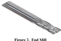
An End mill as shown in Figure 2 is one of the indispensable tools in the milling processing.

Figure 2. End Mill

[image:1.612.382.506.448.532.2]

(2)

International Journal of Emerging Technology and Advanced Engineering

118 The mechanism behind the formation of surface roughness is very dynamic, complicated, and process dependent. Several factors will influence the final surface roughness in a CNC end milling operation such as controllable factors (spindle speed, feed rate and depth of cut) and uncontrollable factors (tool geometry and material properties of both tool and work piece) [2]. Milling is one of the most common process in manufacturing and is very commonly employed in numerical control machines for material removal operations.

Oktem and Erzurumlu [3] observed closeness in the results between experimental and predicted values in end milling process. They used neural network and genetic algorithm. Azlon zain, Haron and sharif [4] observed the effect of different parameter like cutting speed, feed and rake angle in surface roughness. They compared the result of regression modeling and genetic algorithm. I.N. Tansela, et al., [5] have taken three parameters namely cutting speed, feed rate and radial depth of cut for milling process and applied ANN. They obtained good agreement between predicted and actual values.

Hence the optimization of this process is particularly more important to save cost and time. Experimental optimization consisting of suitable selection of machining parameters for End Milling process relies heavily on the operator‟s technologies and experience because of their numerous and diverse range. Machining parameters provided by the machine tool builder cannot meet operator‟s requirements. Since for an arbitrary desired machining time for a particular job, they do not provide the optimal conditions. Therefore there is a need to develop a methodology to optimize the process parameters in End Milling process. The present work involves the estimation of optimal values of the process variables like, speed, feed and depth of cut, whereas the metal removal rate (MRR) and tool wear resistance were taken as the output. Full factorial design was used to carry out the experimental design. Artificial Neural networks (ANN) program available in Matlab software is used to establish the relationships between the input process parameters and the output variables. Later the models given by ANN can be used for optimizing the process.

II. EXPERIMENTAL WORK

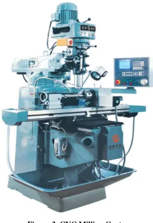
The experiments were conducted on a powerful and precise 3-axis CNC vertical machining center as shown in Figure 3. AISI S2 is taken as the work piece material for investigation.

AISI S2 is a Shock-Resisting Steel grade Tool Steel. It is composed of (in weight percentage) 0.40-0.55% Carbon (C), 0.30-0.50% Manganese (Mn), 0.90-1.20% Silicon (Si), 0.30% Nickel (Ni), 0.30-0.60% Molybdenum (Mo), 0.50% Vanadium (V), 0.25% Copper (Cu), 0.03% Phosphorus (P), 0.03% Sulfur (S), and the base metal Iron (Fe). It has excellent toughness and fine wear resistance and finds various applications in cutting tools for heavy plate, shear blades, cold punching and upsetting and used in various cutting tools.

[image:2.612.365.520.289.515.2]

The specimen is prepared with the dimensions of 150mm x 250mm x 20mm and ceramic insert is used for experimentation.

Figure 3. CNC Milling Centre

Based on the literature survey and the trail experiments, it was found that the process parameters such as spindle speed (x1), feed (x2), and axial depth of cut (x3) were considered as the decision (control) variables and the MRR and the tool wear were considered as the output responses.

[image:2.612.324.576.632.713.2]

The ranges of the process control variables are given in table 1.

Table 1

Range of Cutting parameters used

Input

Variables Units Notation

Feasible range

Lower Limit Upper Limit

Cutting Speed Rpm x1 900 1500

Feed mm/m

in x2 30 60

Depth of Cut mm/m

(3)

International Journal of Emerging Technology and Advanced Engineering

[image:3.612.346.546.119.236.2]

119 After conducting the experiments as per the design matrix, the output responses were measured and recorded and is shown in the Table 2.

Table 2 Experimental dataset

S.No SPEED (X1)

FEED (X2)

DEPTH OF

CUT (X3) M.R.R WEAR

1 1500 30 0.6 5.587 0.163

2 900 30 0.4 3.487 0.09

3 1500 60 0.5 8.294 0.209 4 1200 45 0.6 7.59 0.199 5 1200 30 0.5 4.888 0.13 6 900 30 0.6 5.587 0.139 7 1500 30 0.4 3.492 0.115 8 1200 60 0.4 5.924 0.145 9 900 45 0.4 4.744 0.145 10 1200 45 0.5 6.641 0.174 11 900 45 0.5 6.641 0.149 12 1200 30 0.4 3.497 0.115 13 1200 45 0.4 4.744 0.148 14 1500 45 0.6 7.605 0.207 15 1500 60 0.6 9.479 0.225 16 900 45 0.6 7.59 0.175 17 1500 45 0.4 4.744 0.11 18 900 60 0.6 9.479 0.225 19 900 30 0.5 4.888 0.13 20 1500 30 0.5 4.888 0.116 21 900 60 0.5 8.294 0.189 22 1500 60 0.4 5.924 0.175 23 1200 60 0.5 8.294 0.202 24 1500 45 0.5 6.654 0.188 25 1200 60 0.6 9.479 0.235 26 900 60 0.4 5.924 0.173 27 1200 30 0.6 5.594 0.143

III. MODELING USING ANN

[image:3.612.57.280.185.580.2]

Artificial neural networks are composed on simple elements operating in parallel. These elements are inspired by biological nervous systems and is shown in figure 4.

Figure 4. Biological nervous system

Two different neural network models are used, one for the prediction of MRR and second for the prediction of Tool Wear. The networks were trained with Levenberg-Marquardt algorithm. This training algorithm was chosen due to its high accuracy in similar function approximation [6]. In order to improve the generalization of the network, a „regularization‟ scheme was used in conjunction with the Levenberg-Marquardt algorithm. The automatic Bayesian regularization was used. For training with Levenberg-Marquardt combined with Bayesian regularization, the input/output dataset was divided randomly into two categories: training dataset and test dataset.

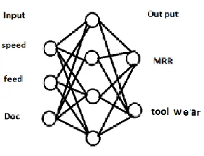
The ANN modeling is carried in two steps; the first step is to train the network whereas the second is to test the network with data, which were not used for training. In this research, a two layer back propagation network was employed as a tool for mapping the complex and highly inter-active process parameters such as Cutting speed, Feed and Depth of Cut.

Figure 5. Layers in Neural Networks

[image:3.612.369.518.485.599.2]

(4)

International Journal of Emerging Technology and Advanced Engineering

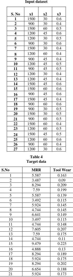
120 Table 3

Input dataset

S. No x1 x2 x3

1 1500 30 0.6

2 900 30 0.4

3 1500 60 0.5

4 1200 45 0.6

5 1200 30 0.5

6 900 30 0.6

7 1500 30 0.4

8 1200 60 0.4

9 900 45 0.4

10 1200 45 0.5

11 900 45 0.5

12 1200 30 0.4

13 1200 45 0.4

14 1500 45 0.6

15 1500 60 0.6

16 900 45 0.6

17 1500 45 0.4

18 900 60 0.6

19 900 30 0.5

20 1500 30 0.5

21 900 60 0.5

22 1500 60 0.4

23 1200 60 0.5

24 1500 45 0.5

25 1200 60 0.6

26 900 60 0.4

[image:4.612.94.243.146.704.2]

27 1200 30 0.6

Table 4 Target data

S.No MRR Tool Wear

1 5.587 0.163

2 3.487 0.09

3 8.294 0.209

4 7.59 0.199

5 5.587 0.139

6 3.492 0.115

7 5.924 0.145

8 4.744 0.145

9 6.641 0.149

10 3.497 0.115

11 4.744 0.148

12 7.605 0.207

13 7.59 0.175

14 4.744 0.11

15 9.479 0.225

16 4.888 0.13

17 8.294 0.189

18 5.924 0.175

19 8.294 0.202

20 6.654 0.188

21 5.924 0.173

Table 5 Testing data

S. No x1 x2 x3

5 1200 30 0.5

10 1200 45 0.5

15 1500 60 0.6

20 1500 30 0.5

25 1200 60 0.6

3.1 ANN model design for prediction of Material Removal Rate (MRR)

The following are the steps involved in the model design for MRR & Tool wear.

Fixing the number of nodes in input and output layers:

The number of input nodes will be equal to the number of inputs i.e., three in this case. Similarly the number of output layer nodes will be equal to the number of outputs i.e., one in this case.

Input and output normalization:

The neural network performance will be good if the input and output values lies in the range [0, 1]. To convert the original inputs and outputs into the required form the following equations are developed.

Mi = Ai/Maxi ; Mo = Ao/Maxo

Fixing the number of hidden layers:

Generally single and double hidden layers networks are used to solve the most of the problems. Here also single hidden layer is verified. Double hidden layer has given the minimum error than the single hidden layer.

Network model for MRR:

Network type: feed forward back propagation Training: Levenberg Maquardtl algorithm No. of layers: 2

Output layer: 1 No of neurons: 0 to10

Performance: mean square error

Training function: TRAINLM of the network Hidden layer transfer function: Tran sigmoid Output layer transfer function: Pure linear Adaption of learning rate: LEARNGDM

(5)

International Journal of Emerging Technology and Advanced Engineering

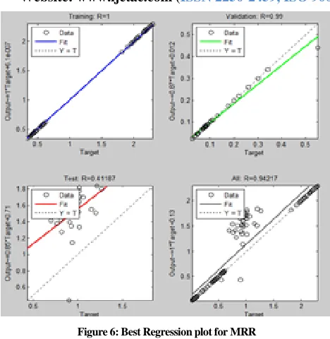
[image:5.612.332.552.125.377.2]

121 Figure 6: Best Regression plot for MRR

Fixing the number of nodes in each hidden layer:

[image:5.612.50.284.127.367.2]

The number of hidden layer nodes can be fixed based on the minimum error. In this case the error is minimum at 8 nodes in first hidden layer and 4 nodes in second hidden layer.

Table 6

Best performance error with hidden nodes for MRR

Hidden Layer Best performance error

2 0.012

5 0.098

10 0.0018

15 0.031

20 0.062

Network model for Tool Wear Resistance:

Network type: feed forward back propagation Training: Levenberg Maquardtl algorithm No. of layers: 2

Output layer: 1 No of neurons: 0 to20

Performance: mean square error

Training function: TRAINLM of the network Hidden layer transfer function: Tran sigmoid Output layer transfer function: Pure linear Adaption of learning rate: LEARNGDM

No of epoch of the network: 84 epochs will get good results and best regression plot.

Figure 7: Best Regression plot for Tool wear

Fixing the number of nodes in each hidden layer:

[image:5.612.71.266.451.521.2]

The number of hidden layer nodes can be changed up to getting minimum error in the best performance. It is single hidden layer and changing the nodes in the hidden layer. Best performance error is less at nodes 17and the 18.

Table 7

Best performance error with hidden nodes for Tool wear

Hidden Layer Best performance error

16 0.0272

17 0.0123

18 0.0043

19 0.076

20 0.0987

IV. RESULTS &DISCUSSION

[image:5.612.339.546.464.572.2]

(6)

International Journal of Emerging Technology and Advanced Engineering

122 Figure 8: Experimental & Predicted MRR values

Figure 9: Experimental & Predicted Tool Wear values

V. CONCLUSIONS

In this work, experiments were conducted on a powerful and precise 3-axis CNC vertical machining center, mode employing employing a continuously variable spindle speed up to a maximum of 6000 rpm and with a maximum spindle power of 5.5kW. The feed rates can be set up to a maximum of 10m/min. Experiments were conducted as per the deign matrix. Cutting speed, Feed and Depth of cut were taken as the process parameters and the output responses i.e Material removal rate and Tool wear resistance were taken as the output responses.

Full factorial design was used to carry out the experimental design. Artificial Neural networks (ANN) program available in Matlab software is used to establish the relationships between the input process parameters and the output variables. The models were developed to predict the MRR and Tool wear resistance through Artificial Neural Networks techniques. The best model is selected based on the best performance error for different network configurations. Also the models have been evaluated by means of the percentage deviation between the predicted values and the actual values. Also the graphs were plotted between the measured values and the ANN predicted results. It is shown that the ANN predicted results shows good agreement with the Experimental results, Hence ANN proved its efficiency in optimizing the End Milling process parameters. The developed ANN model can be further integrated with optimization algorithms like GA to optimize the End milling parameters.

REFERENCES

[1 ] Mike S. Lou., Joseph C. Chen., and Caleb M. Li.,1999. Surface roughness prediction technique for CNC end milling. Journal of Industrial Technology, Vol.17, No. 2-7, pp. 2-6

[2 ] Optimization of Cutting Conditions in End Milling Process with the Approach of Particle Swarm Optimization Vikas Pare, Geeta Agnihotri & C.M. Krishna Mechanical Engineering Department, Maulana Azad National Institute of Technology, Bhopal, India [3 ] Oktem and Erzurumlu 2006 “Prediction of minimum surface

roughness in end milling mold parts using neural network and genetic algorithm” Vol 27,pp 735-744

[4 ] Haron and Shariff (2010) “Application of GA to optimize cutting condition for minimizing surface roughness in end milling machining process”,Vol37,pp 4650-4659 I.N.

[5 ] Tansela,W.Y. Baoa, N.S. Reena, C.V. Kropas-Hughesb ,Genetic tool monitor (GTM) for micro-end-milling operations Oct2004. International Journal of machine tools &manufacture, volume 45, issue 3