Data analytics enhanced component volatility model

(1)

D a t a a n a ly ti c s e n h a n c e d

c o m p o n e n t vol a tility m o d e l

Yao, Y, Z h a i, J, C a o , Y, Di n g , X, Li u, J a n d L u o, Y

h t t p :// dx. d oi.o r g / 1 0 . 1 0 1 6 /j. e s w a . 2 0 1 7 . 0 5 . 0 2 5

T i t l e

D a t a a n a ly ti c s e n h a n c e d c o m p o n e n t vol a tility m o d el

A u t h o r s

Yao, Y, Z h ai, J, C a o , Y, Di n g , X, Liu, J a n d L u o, Y

Typ e

Ar ticl e

U RL

T hi s v e r si o n is a v ail a bl e a t :

h t t p :// u sir. s alfo r d . a c . u k /i d/ e p ri n t/ 4 2 3 1 4 /

P u b l i s h e d D a t e

2 0 1 7

U S IR is a d i gi t al c oll e c ti o n of t h e r e s e a r c h o u t p u t of t h e U n iv e r si ty of S alfo r d .

W h e r e c o p y ri g h t p e r m i t s , f ull t e x t m a t e r i al h el d i n t h e r e p o si t o r y is m a d e

f r e ely a v ail a bl e o nli n e a n d c a n b e r e a d , d o w nl o a d e d a n d c o pi e d fo r n o

n-c o m m e r n-ci al p r iv a t e s t u d y o r r e s e a r n-c h p u r p o s e s . Pl e a s e n-c h e n-c k t h e m a n u s n-c ri p t

fo r a n y f u r t h e r c o p y ri g h t r e s t r i c ti o n s .

(2)

1

Data analytics enhanced component volatility model

Author:

Yuan Yao

Institute of Management Science and Engineering, Business School,

Henan University, 475004, Jinming District, Kaifeng, Henan Province, China [email protected]

Jia Zhai

Salford Business School, University of Salford,

43 Crescent, Salford M5 4WT, UK [email protected]

[email protected]

Yi Cao

Department of Business Transformation and Sustainable Enterprise, Surrey Business School, University of Surrey,

Guildford, Surrey, GU2 7XH, United Kingdom

[email protected]

Xuemei Ding

School of Computing and Intelligent Systems, Ulster University, Magee campus,

Northland Rd, Londonderry Northern Ireland, UK, BT48 7JL [email protected]

Faculty of Software, Fujian Normal University, Upper 3rd Rd, Cangshan, Fuzhou,

(3)

2 Junxiu Liu,

School of Computing and Intelligent Systems, Ulster University, Magee campus,

Northland Rd, Londonderry Northern Ireland, UK, BT48 7JL [email protected]

Yuling Luo

Guangxi Key Lab of Multi-Source Information Mining & Security, Faculty of Electronic Engineering, Guangxi Normal University, Diecai, Guilin, Guangxi, China, 541000

[email protected]

Corresponding author:

Jia Zhai

Salford Business School, University of Salford,

43 Crescent, Salford M5 4WT, UK +44(0) 161 295 8147

(4)

3

Data analytics enhanced component volatility model

Abstract

Volatility modelling and forecasting have attracted many attentions in both finance and computation areas. Recent advances in machine learning allow us to construct complex models on volatility forecasting. However, the machine learning algorithms have been used merely as additional tools to the existing econometrics models. The hybrid models that specifically capture the characteristics of the volatility data have not been developed yet. We propose a new hybrid model, which is constructed by a low-pass filter, the autoregressive neural network and an autoregressive model. The volatility data is decomposed by the low-pass filter into long and short term components, which are then modelled by the autoregressive neural network and an autoregressive model respectively. The total forecasting result is aggregated by the outputs of two models. The experimental evaluations using one-hour and one-day realized volatility across four major foreign exchanges showed that the proposed model significantly outperforms the component GARCH, EGARCH and neural network only models in all forecasting horizons.

1. Introduction

(5)

4 has been proposed to capture the long memory property in realized volatility (Granger C. W., 1980) (Granger & Joyeux, 1980). In 1999, (Lee & Engle, 1999) introduced a component GARCH model, which decomposes volatility into two components: a permanent long run trend component and a transitory short-run one that is mean-reverted to the long-run trend (Harris, Stoja, & Yilmaz, 2015). After that, more empirical evidences suggested that two-component model can capture the volatility structure much better than the one-component models. For example, (Brandt & Jones, 2006) showed that daily volatility can be well characterized by two-component model structure with one highly persistent two-component and one strongly stationary two-component. A number of literatures have found that two-component volatility models perform better than the one-component models in explaining stock as well as exchange rate volatilities. Started from one-component GARCH model, introduced by (Lee & Engle, 1999), those two-component models usually consider the volatilities as a composition of a permanent long-run trend component and a transitory short-run component, both of which follow a mean-reverting process with a slow reversion speed in long-run trend and quick reversion speed in the short-run one.

(6)

(7)

6 trend or the seasonality, can dramatically reduce forecasting errors and is critical to build an adequate ARNN based forecasting model.

(8)

7 long horizon forecasting. Overall, the experimental evaluations show that our proposed model achieves a stable and much better forecasting performance than most of the traditional volatility models.

The outline of the remainder of this paper is as follows. In Section 2, we present the structure and details of the proposed model. Section 3 describes the data used in the empirical analysis and the forecasting evaluation criteria. Section 4 presents the empirical results and Section 5 provides a summary, concluding remarks and some future research directions.

2. Methodology

2.1 Model structure

In this paper, we follow this idea and the model format in (Lee & Engle, 1999), we assume the realized volatility follows a two-component process given by

σt= 𝐿𝑡+ 𝑆𝑡 (1)

𝑆_𝑡 = 𝛼𝑆_𝑡−1+ ε_t (2)

where 𝐿_𝑡 and 𝑆_𝑡 are the long and short term component of the realized volatility respectively and ε_t is the random error term with zero mean and constant variance. The short term component 𝑆𝑡 is an autoregressive,

AR(1), process with the parameter 𝛼, which measures the speed of the short term revision to long term trend. This structure of the volatility is following the two-component characteristics in previous literatures, for example (Lee & Engle, 1999), (Alizadeh, Brandt, & Diebold, 2002), and (Brandt & Jones, 2006). However, the implementation of our two-component model is different from traditional Component GARCH model.

(9)

8 (Hodrick & Prescott, 1997). After getting 𝐿𝑡, the short term component of the realized volatility can be

obtained by 𝑆_𝑡= σ_t− 𝐿_𝑡. In the second step, we train an artificial neural network (ANN) using the long-term component 𝐿_𝑡 to obtain a forecasting model. A future value of 𝐿_𝑡+𝑛 at time 𝑡 + 𝑛 can be forecasted by the trained ANN. In the last step, the AR(1) process model 𝑆𝑡 = 𝛼𝑆𝑡−1+ εt is estimated using the short term

component 𝑆_𝑡, which is obtained from the first step. A future value of 𝑆_𝑡+𝑛 at time 𝑡 + 𝑛 can be then forecasted by the estimated AR(1) model. Therefore, we can calculate the future value of the realized volatility at time 𝑡 + 𝑛 by 𝜎_𝑡+𝑛 = 𝐿_𝑡+𝑛+ 𝑆_𝑡+𝑛.

2.2 Volatility decomposition

In the first step, the long-term component 𝐿_𝑡 is extracted from the realized volatility. To do this, the low-pass Hodrick-Prescott filter (Hodrick & Prescott, 1997) is applied to extract a low frequency non-linear component from a time-series. That low frequency component represents the trend of the long-term component of the realized volatility. Hodrick-Prescott filter (Hodrick-Prescott filter) is widely used in applied macroeconomics (Stock & Watson, 1999) (McElroy, 2008) (Stock & Watson, 2016) for removing the short-term cyclical component of a time series from raw data. Given the value of the smoothing parameter 𝜆, the long term trend component shall solve

min

𝜏 (∑(𝑦𝑡 − 𝜏𝑡)

2_{+ 𝜆 ∑[(𝜏}

𝑡+1− 𝜏𝑡) − (𝜏𝑡− 𝜏𝑡−1)]2 𝑇−1

𝑡=2 𝑇

𝑡=1

)

(10)

9

2.3 Autoregressive Neural Network

2.3.1 Network structure

In the second step of implementing our two-component model, we use an autoregressive neural network (ARNN), a special format of artificial neural network, to model and forecasting the long-term component 𝐿𝑡

of realized volatility. As the discussion in Section 1, the work in (Sharda & Patil, Oct 1992) (Gorr, June 1994) (Zhang & Qi, 16 January 2005) show that ARNN outperforms other structure of artificial neural network in trend and seasonality forecasting of a non-linear time series. (Zhang & Qi, 16 January 2005) and (Nelson, Hill, Remus, & O'Connor, 1999) further show that prior data processing, removing either the trend or the seasonality, can dramatically reduce forecasting errors and is critical to build an adequate ARNN based forecasting model. Therefore, in our paper, we follow the existing study and employ the ARNN to model and forecasting the trend, the long-term component 𝐿_𝑡 of realized volatility. The reason of selecting ARNN is twofold. First, main strand finance literature usually assumes the volatility is composed of two autoregressive process, long term and short term. We follow the traditional assumption with augmented adjustment: ARNN, which models the lags as a nonlinear function. Secondly, compared with other artificial neural network, ARNN can achieve even better accuracy in “deseasonalized” financial time-series forecasting by a relatively simple structure, where appropriate lags instead of a number of additional features is crucial for the forecasting performance. ARNN is also proved to have advantages over recurrent feed-forward neural network and is less sensitive to the problem of long-term dependence (Mustafaraj, Lowry, & Chen, 2011). Compared with traditional feed-forward artificial neural network, the ARNN has interconnection from the lagged input to the output layer, which enhances its capability of forecasting more than one-step as a time-series predictor. We follow the traditional ARNN structure:

𝑌_𝑡= 𝛼₀+ ∑ 𝛼_𝑖𝑌_𝑡−𝑖

𝑛

𝑖=1

+ ∑ Ψ (𝛾_0𝑗+ ∑ 𝛾_𝑖𝑗𝑌_𝑡−𝑖

𝑛

𝑖=1

) 𝛽_𝑗

ℎ

𝑗=1

+ 𝜀_𝑡

(11)

non-10 linear part contains ℎ hidden neurons transforms the input variables, defined as the 𝑛-lagged long-term component 𝐿𝑡 of realized volatility, weighted by parameters 𝛾𝑖𝑗 plus a bias 𝛾0𝑗, via a non-linear activation

function Ψ(. ). If representing the number of lags and hidden neurons as 𝑖 and 𝑗, a hidden neuron can be denoted by

Ψ (𝛾_0𝑗+ ∑ 𝛾_𝑖𝑗𝑌_𝑡−𝑖

𝑛

𝑖=1

)

each of which is weighted by a parameter 𝛽𝑗 before it produces the output layer. Since we want to model and

forecasting the long-term component of volatility, ARNN operates as a non-linear regression function at the end as

𝑌_𝑡 = 𝐺(𝑌_𝑡−1, 𝑌_𝑡−2, … , 𝑌_𝑡−𝑛) + 𝜀𝑡,𝐴𝑅𝑋𝑁𝑁

(12)

11 and validation dataset are monitored at the same time. When the validation error rises while the training error maintains, the ARNN begins to overfit the data. The weights and bias at the minimum of the validation error are saved as the trained ARNN

2.3.2 Network parameters

Under this structure of ARNN, the number of lags 𝑛 and the number of hidden neurons ℎ are the crucial parameters for constructing the ARNN model. We follow the widely used configuration for the ARNN in (Siegelmann, Horne, & Giles, 1997 ) and (Mustafaraj, Lowry, & Chen, 2011), and investigate the performance using the number of lags from 2 to 5, which is 𝑛 = 2,3,4,5. We firstly use ℎ = 10 as the preliminary configuration for the number of hidden neurons and finds the appropriate lags. We use the long-term component 𝐿𝑡 of one hour realized EURUSD rate from 27 Sep 2009 to 06 Dec 2012 to train the ARNN

model under 𝑛 = 2,3,4,5 and use 500 long-term component values of EURUSD rate from 07 Dec 2012 to 15 Jan 2013 to test the trained model. The forecasting error is defined as 𝐿̂_𝑡− 𝐿_𝑡, the difference between the original value 𝐿𝑡 and the forecasted one. The average errors across the forecasting horizons is listed in Table

1, where we can observe that the best average error is at 𝑛 = 4, although the errors do not show a significant difference among different configuration of lag numbers. Four lags also conform to the configuration suggested in (Siegelmann, Horne, & Giles, 1997 ) and (Mustafaraj, Lowry, & Chen, 2011). Therefore, in this paper, we use four lags autoregressive neural network (ARNN) following the suggested configuration and our empirical investigation.

Table 1 This table contains the average forecasted error across the horizon from 07 Dec 2012 to 15 Jan 2013 under configurations of lag number from 2, 3, 4 and 5

𝑛 = 2 𝑛 = 3 𝑛 = 4 𝑛 = 5 Average error 1.22807E-05 1.22647E-05 1.21385E-05 1.2293E-05

(13)

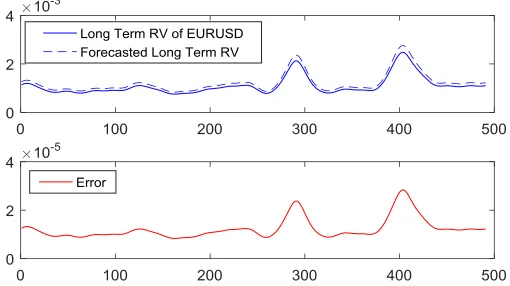
12 𝐿𝑡 of EURUSD rate from 27 Sep 2009 to 06 Dec 2012. The forecasting results 𝐿̂𝑡 include 500 long-term

[image:13.612.112.367.190.333.2]

component values of EURUSD rate from 07 Dec 2012 to 15 Jan 2013. The forecasting error, defined as 𝐿̂_𝑡− 𝐿_𝑡, between the original value 𝐿_𝑡 and the forecasted one 𝐿̂_𝑡 are shown in the bottom sub-figure, from which we can observe that out-of-sample forecasting errors are around 10−5_.

Figure 1 This figure shows an example of out-of-sample forecasting long term component 𝑳𝒕 of EURUSD using ARNN. The top

figure shows the long term component of EURUSD from 07 Dec 2012 to 05 Feb 2013 decomposed by Hodrick-Prescott filter. The middle figure shows the forecasted value 𝑳̂𝒕of the long term component of EURUSD from 07 Dec 2012 to 15 Jan 2013 using ARNN

model. The bottom figure shows the differences 𝑳̂𝒕− 𝑳𝒕between the original long term component of EURUSD and the forecasted one.

2.4 Autoregressive model

In the third step, we estimate an autoregressive model for the short-term component 𝑆𝑡: 𝑆𝑡 = 𝛼𝑆𝑡−1+ εt. The

n-step ahead forecasting of the short-term component 𝑆𝑡 is therefore given by

𝑆̂_𝑡+𝑛 = 𝛼𝑛_𝑆

𝑡+ ∑𝑛−1𝑖 𝛼𝑖εt−i (3)

We can obtain the forecasted the long-term component 𝐿̂𝑡+𝑛 of the realized volatility through ARNN model.

(14)

13 model for the short-term component 𝑆𝑡, we utilize the method of moment through Yule–Walker equations,

named for Udny Yule and Gilbert Walker (Yule, 1927) (Walker, 1931):

𝛾_𝑚= ∑ 𝛼_𝑘𝛾_𝑚−𝑘

𝑝

𝑘=1

+ 𝜎_𝜖2_𝛿 𝑚,0

where 𝛾𝑚 is the autocovariance function of 𝑆𝑡, 𝜎𝜖2 is the variance of the input noise process and the 𝛿𝑚,0 is

the Kronecker delta function. For the case 𝑝 = 1, one lag autoregressive process AR(1), the 𝛼₁ can be obtained by 𝛾₁/𝛾₀.

2.5 Model flow

We summarize the NNE2C model workflow when applied in realized volatility forecasting. Different from other hybrid models, which usually use the neural network as the dominate one to model the non-linear part of the underline financial variable, i.e. volatility or foreign exchange and use the ARIMA (McDonald S. , Coleman, McGinnity, Li, & Belatreche, 2014) or GARCH model (Kristjanpoller, Fadic, & Minutolo, 2014) as the pre-processing part for modelling the linear part of the underline financial variable, the NNE2C model follows the traditional financial theory to consider the volatility as a combination of the long and short term while producing an enhanced mechanism through explicitly decomposing the two components and modelling them separately. The simple NNE2C model follows and enhances the financial theory by capturing the volatility structure explicitly and effectively.

Algorithm 1 Workflow of proposed NNE2C model

1 Given the realized volatility σt of selected financial security, i.e. FX, we assume it is composed of long and short term components: σt= 𝐿𝑡+ 𝑆𝑡

2 We use Hodrick-Prescott filter as a low-pass filter to explicitly extract the long term component 𝐿𝑡. The smoothing parameter 𝜆 of Hodrick-Prescott filter is selected according to the empirical study: 𝜆 = 100 ∗ (360 ∗ 8)2₌ 829440000.

min

𝜏 (∑(σt− 𝜏𝑡)

2_{+ 𝜆 ∑[(𝜏}

𝑡+1− 𝜏𝑡) − (𝜏𝑡− 𝜏𝑡−1)]2 𝑇−1

𝑡=2 𝑇

𝑡=1

)

(15)

14 Using 𝐿𝑡 to train the ARNN with 4 lags and 10 hidden neurons, 𝑛 step ahead 𝐿𝑡+𝑛 is forecasted by the trained ARNN model;

𝐿𝑡= 𝛼0+ ∑ 𝛼𝑖𝐿𝑡−𝑖 𝑛

𝑖=1

+ ∑ Ψ (𝛾0𝑗+ ∑ 𝛾𝑖𝑗𝐿𝑡−𝑖 𝑛

𝑖=1

) 𝛽𝑗 ℎ

𝑗=1

+ 𝜀𝑡

Using 𝑆𝑡 to estimate the AR(1) model, 𝑛 step ahead 𝑆𝑡+𝑛 is forecasted by the estimated AR(1) model; 𝑆𝑡= 𝛼𝑆𝑡−1+ εt

5 𝑛 step ahead realized volatility is obtained by σt+n= 𝐿𝑡+n+ 𝑆𝑡+n

3. Data and forecasting evaluation

3.1 Data

We use the neural network enhanced two-component model defined in Section 2 to forecasting the volatility of the EUR/USD, GBP/EUR, GBP/JPY and GBP/USD exchange rates. High frequency exchange rate data (tick data) were obtained from Oricode Inc for the period 27 September 2009 to 12 August 2015 and included around 7.7 billion observations across 2145 days. The unobserved true volatility, in principle, can be estimated arbitrarily accurately using a measure of realized volatility calculated through the intraday returns (Harris, Stoja, & Yilmaz, 2015). It is proved by (Torben, Tim, & Francis, 2009) that the sum of squared intraday returns converges to the unobserved true volatility with the intraday interval approaching to zero. In this study, we use realized volatility as the proxy of the unobserved true volatility. This is obtained by aggregating the intraday squared returns using the approach given by (Andersen & Bollerslev, 1998):

𝜎̂_{𝑟𝑣,𝑡}2 _{= ∑ 𝑟} 𝑡,𝑛2 𝑁

𝑛=1

where 𝜎̂_{𝑟𝑣,𝑡}2 _{is the realized volatility for time 𝑡, and 𝑟}

𝑡,𝑛2 is the squared log return on time 𝑡 for interval 𝑛 (𝑛 =

1,2, … , 𝑁). In this paper, we use one-hour and one-day realized volatilities, both of which are constructed

from 10 millisecond log return, which is the highest frequency in our data.

The one-hour realized volatility is obtained by aggregating 360,000 10-millisecond log returns 𝑟_𝑡,𝑛2 _{in each}

(16)

15 estimation of the model, while the data from 08 December 2012 to 12 August 2015 (16681) is used for out-of-sample evaluation. The one-day realized volatilities is constructed by the sum of 3,600,000 log returns in each trading day. For the one-day realized volatilities, the data from 27 September 2009 to 07 December 2012 (1000 observations) is used for the initial estimation of the model, while the remained data (837 observations) is used for out-of-sample evaluation.

[image:16.612.81.502.403.678.2]

Table 2 reports summary statistics for the one-hour and one-day realized volatilities of full observations of four exchange rates. Panel A reports the mean, standard deviation, skewness and excess kurtosis and Bera– Jarque statistic and Panel B reports the first six autocorrelation coefficients and the Ljung–Box Q statistic for autocorrelation of six lags for the realized volatilities. P-values are also reported in parentheses. In the Ljung– Box Q tests, the null hypothesis that the residuals of the returns are not autocorrelated is rejected in both one-hour and one-day realized volatilities. Therefore the two realized volatilities are all highly autocorrelated.

Table 2 Summary statistics and autocorrelations

mean Standard deviation Skewness Excess kurtosis Bera-Jarque Panel A: Summary statistics

GBP/USD 1 Hr 1.6657E-06 9.1010E-06 1.0231E+02 1.1661E+04 2.0743E+11 GBP/JPY 1 Hr 3.6200E-06 7.6346E-06 4.5817E+01 3.4566E+03 1.8227E+10 GBP/EUR 1 Hr 1.8514E-06 3.1560E-06 2.5651E+01 1.1853E+03 2.1401E+09 EUR/USD 1 Hr 2.1207E-06 5.6940E-06 4.4465E+01 3.8006E+03 2.2055E+10

GBP/USD Daily 3.2698E-05 7.2746E-05 3.5359E+01 1.4143E+03 1.5292E+08 GBP/JPY Daily 7.0981E-05 6.8848E-05 7.5062E+00 1.0538E+02 8.2050E+05 GBP/EUR Daily 3.6060E-05 2.4165E-05 2.4964E+00 1.6728E+01 1.6342E+04 EUR/USD Daily 4.1188E-05 5.5114E-05 2.1497E+01 7.0608E+02 3.8019E+07

Panel B: Autocorrelations

1 2 3 4 5 6 Ljung–Box Q

GBP/USD 1 Hr 0.6638 0.2696 0.0387 0.0210 0.0216 0.0225 1.8952E+04 (0.0000) GBP/JPY 1 Hr 0.2870 0.1879 0.1897 0.1569 0.1559 0.1502 1.4856E+04 (0.0000) GBP/EUR 1 Hr 0.2381 0.1711 0.1363 0.1149 0.0903 0.0784 5.8392E+03 (0.0000) EUR/USD 1 Hr 0.3683 0.2986 0.2442 0.2361 0.1952 0.1588 1.7166E+04 (0.0000)

(17)

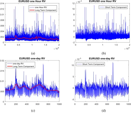
16 In the example in the following Figure 2(a-b), Hodrick-Prescott filter is applied to one hour realized volatility with smoothing parameter 𝜆 of 829440000 (blue curve in Figure 2(a)) of EURUSD exchange rate from 27 Sep 2009 to 07 Dec 2012 to extract the long term component 𝐿_𝑡 (red curve in Figure 2(b)). Figure 2(c-d) shows an example of one-day realized volatility with long term component extracted by Hodrick-Prescott filter with smoothing parameter 𝜆 of 12960000 (assuming 360 trading days per year, the 𝜆 is calculated by 100 multiplied by the squared frequency of the data).

(a) (b)

(c) (d)

Figure 2 (a) Blue curve in the figure: One-hour realized volatility of EURUSD exchange rate from 27 Sep 2009 to 07 Dec 2012; Red curve: the long term component 𝑳𝒕of the realized volatility extracted by low-pass Hodrick-Prescott filter; (b) Short term component

of one-hour realized volatility of EURUSD exchange rate; (c) Blue curve in the figure: one-day realized volatility of EURUSD exchange rate from 27 Sep 2009 to 07 Dec 2012; Red curve: the long term component 𝑳𝒕of the realized volatility extracted by

[image:17.612.95.516.232.596.2]

(18)

17

3.2 Forecasting evaluation

The proposed neural network enhanced two-component model is used to calculate out-of-sample forecastings of the realized volatilities of up to 500 hours or days ahead across the evaluation period for the one-hour or one-day realized volatility respectively. As the benchmark, we select one-factor EGARCH and two-factor Component GARCH of (Lee & Engle, 1999). In addition, we also employ four lags autoregressive neural network applied directly on realized volatility as one of the benchmark models. We therefore estimate four models: a) four lags autoregressive neural network enhanced two-component model (NNE2C); b) one-component EGARCH model; c) two-one-component GARCH model; and d) four lags autoregressive neural network model (NNOnly). The four models are evaluated using one-hour and one-day realized volatilities respectively. For one-hour and one-day data, four models are initially estimated using the first 20,000 and 1,000 observations from 27 Sep 2009 to 07 Dec 2012 respectively and then the volatilities at different estimation periods are calculated. Following (Michael & Christopher, 2006), we consider forecasting horizons of 5, 20, 100, 200, 360, and 500 hours or days ahead for one-hour or one-day volatility respectively. We choose the root mean square error (RMSE) with respect to the true realized volatility as the measure of the forecasting performance:

𝑅𝑀𝑆𝐸 = [1_𝑇∑ (𝜎𝑡(𝜏𝑡, 𝜏𝑡+𝑇) − 𝜎̂𝑡(𝜏𝑖,𝑡, 𝜏𝑡+𝑇)) 2 𝑇

𝑡=1 ]

1 2

(4)

For the shorter evaluation horizons of 5, 20, 100, we calculate the RMSE over the forecasting horizon, i.e. (𝜏_𝑡, 𝜏_𝑡+𝑇) = (1,5), (1,20) and (1,100). For the three longer horizons, we calculate the RMSE over 100 time

points, i.e. (𝜏𝑡, 𝜏𝑡+𝑇) = (100,200), (260,360) and (400,500). For the one-hour realized volatility, the

(19)

18

4. Results

4.1 Model parameter

[image:19.612.86.540.686.720.2]

In theory, three-layer autoregressive neural network can approximate most of the functions as long as a sufficient number of hidden neurons is provided. In this paper, we construct the NNE2C with 5, 10, and 15 neurons in the hidden layer and test the forecasting performance of the proposed model. The results are illustrated in Table 3 and Table 4 for one-hour and one-day realized volatility data respectively. For the comparison purpose, we also included the forecasting results with 10 hidden neurons in Table 3 and Table 4. From Table 3, it is very clear that for the NNE2C, the forecasting accuracies are roughly the same by using different number of hidden neurons. The forecasting accuracy does not increase with the number of hidden neuron increases. This result is consistent in all forecasting horizons across four currencies. The only case that the forecasting accuracy rises with the increase of the number of hidden neurons is highlighted in Table 3 as GBP/USD rate at (100,200) horizon. However, the accuracy increase is as subtle as around 10E-8. For all the cases in Table 4, the forecasting accuracy differences by different number of hidden neurons are also tiny. The only three cases that the forecasting accuracy increases (although tiny) with the rise of the number of hidden neurons are highlighted in Table 4: GBP/JPY rate at horizon (260,360), (400,500) and GBP/EUR at horizon (400,500). In addition, the forecasting accuracies of NNOnly model with different number of hidden neurons do not show significant differences in Table 3 and Table 4 as well. Our results also conform to the previous researches in (Kristjanpoller & Minutolo, 2016) and (Kristjanpoller, Fadic, & Minutolo, 2014). Therefore, based on our experimental evaluations in Table 3 and Table 4, we believe our proposed NNE2C can achieve the best forecasting performance under the structure of three-layer autoregressive neural network with 10 hidden neurons.

Table 3 Forecasting performance of one-hour realized volatilities. This table reports theRoot mean square error (RMSE) for the autoregressive neural network enhanced two-component model constructed by one hidden layer with 5 and 15 neurons (NNE2C) and autoregressive neural network model constructed by one hidden layer with 5, 10 and 15 neurons (NNOnly).

𝜏₁ 𝜏₂ NNE2C

(5 neurons)

NNE2C

(10 neurons)

NNE2C

(15 neurons)

NNOnly

(5 neurons)

NNOnly

(10 neurons)

NNOnly

(15 neurons)

(20)

19 GBP / EUR 9.8432E-06 9.8434E-06 9.8435E-06 7.5266E-02 7.4758E-02 7.4355E-02

GBP / JPY 4.9453E-05 4.9452E-05 4.9452E-05 1.4364E-01 1.3907E-01 1.4022E-01 GBP / USD 1.1083E-05 1.1081E-05 1.1087E-05 5.5426E-02 5.2369E-02 5.4421E-02

1 20 EUR / USD 5.7274E-05 5.7239E-05 5.7276E-05 1.3165E-01 1.3015E-01 1.3121E-01 GBP / EUR 4.8869E-05 4.8870E-05 4.8870E-05 1.2097E-01 1.2032E-01 1.2054E-01 GBP / JPY 5.3459E-05 2.3459E-05 5.3459E-05 1.5310E-01 1.4879E-01 1.5035E-01 GBP / USD 2.6065E-05 2.6063E-05 2.6069E-05 7.4815E-02 7.2129E-02 7.3733E-02

[image:20.612.87.537.462.718.2]

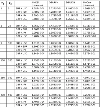
Table 4 Forecasting performance of one-day realized volatilities. This table reports theRoot mean square error (RMSE) for the autoregressive neural network enhanced two-component model constructed by one hidden layer with 5 and 15 neurons (NNE2C) and autoregressive neural network model constructed by one hidden layer with 5 and 15neurons (NNOnly)

𝜏₁ 𝜏₂ NNE2C

(5 neurons)

NNE2C

(10 neurons)

NNE2C

(15 neurons)

NNOnly

(5 neurons)

NNOnly

(10 neurons)

NNOnly

(15 neurons)

1 20 EUR / USD 1.7691E-04 1.7692E-04 1.7702E-04 5.7042E-01 5.7113E-01 5.7226E-01 GBP / EUR 1.3060E-04 1.3087E-04 1.3088E-04 4.4148E-01 4.3658E-01 4.4204E-01 GBP / JPY 2.2931E-04 2.2910E-04 2.3074E-04 7.8099E-01 7.7768E-01 7.8039E-01 GBP / USD 3.4261E-04 3.4074E-04 3.4227E-04 1.4302E+00 1.4300E+00 1.4300E+00

(21)

20 260 360 EUR / USD 1.3838E-04 1.3791E-04 1.4283E-04 4.2934E-01 4.3042E-01 4.3157E-01

GBP / EUR 1.6731E-04 1.6787E-04 1.6194E-04 5.2557E-01 5.2051E-01 5.2631E-01 GBP / JPY 2.0534E-04 2.0251E-04 1.7687E-04 6.4310E-01 6.3951E-01 6.4250E-01 GBP / USD 1.3880E-04 1.3370E-04 1.3637E-04 4.2614E-01 4.2548E-01 4.2597E-01

4.2 Experimental results

Following the configurations, we employ our experiments using NNE2C with 4 lags and 10 neurons. Table 5 and Table 6 report the RMSE of the one-hour and one-day realized volatilities given by equation (4) for four models over six forecasting intervals for four currencies respectively. Overall, for all models in the experiments in Table 5 and Table 6, the RMSE measures fall at the first with the forecasting horizon and then rise for four currencies. This is due to the reason that initially the forecasting interval increases from five to 20 and then to 100 time points. After the horizon (𝝉𝒕, 𝝉𝒕+𝑻) = (𝟏, 𝟏𝟎𝟎), the forecasting interval is fixed at

100 time points, and therefore the forecasting error rises as the horizon increases.

In one-hour realized volatility evaluations in Table 5, the NNE2C model shows the highest forecasting accuracy in 23 out of 24 cases (four currencies with each having 6 horizons) followed by CGARCH model. The only exception is the highlighted case in Table 5: CGARCH achieved RMSE of 3.2067E-05 at horizon (𝟏𝟎𝟎, 𝟐𝟎𝟎) on GBP/EUR and was more accurate than the NNE2C, which had 3.2874E-05 RMSE at the same case. At horizon of (𝟏, 𝟏𝟎𝟎), the performance of CGARCH model is lower but close to the performance of the NNE2C in all four currencies. In other horizons, the NNE2C is significantly more accurate than CGARCH model. Particularly, the decline of the forecasting accuracy of the CGARCH model as well as EGARCH and NNOnly model is obvious from horizon (𝝉𝒕, 𝝉𝒕+𝑻) = (𝟏𝟎𝟎, 𝟐𝟎𝟎) to (𝟐𝟔𝟎, 𝟑𝟔𝟎) and then to

[image:21.612.84.534.71.177.2]

(𝟒𝟎𝟎, 𝟓𝟎𝟎). It shows that at longer forecasting horizon, the NNE2C has sufficiently stronger forecasting capability than the traditional models.

(22)

21

neurons), Component GARCH model, EGARCH model, and autoregressive neural network model (NNOnly), for the forecasting interval 𝝉𝟏 to 𝝉𝟐, where 𝝉𝟏= 𝒎𝒂𝒙(𝟏, 𝝉𝟐− 𝟏𝟎𝟎), for the one-hour realized volatilities of four currencies.

𝜏1 𝜏2 NNE2C

(10 neurons)

CGARCH EGARCH NNOnly

(10 neurons)

1 5 EUR / USD 3.0167E-06 5.1341E-04 8.1872E-04 5.8289E-02 GBP / EUR 9.8434E-06 1.7790E-04 5.8565E-04 7.4758E-02 GBP / JPY 4.9452E-05 1.9269E-04 1.0531E-03 1.3907E-01 GBP / USD 1.1081E-05 3.2305E-04 6.4933E-04 5.2369E-02

In Table 6, the NNE2C was significantly more accurate than other three models in all 24 cases. In the highlighted cases in Table 6, which include GBP/EUR rate at (1,5) and (1,20) horizons, and GBP/EUR rate at (400,500) horizon, CGARCH model achieved the forecasting accuracies lower but close to the performance of the NNE2C. In other cases, the NNE2C remarkably outperforms all other models.

(23)

[image:23.612.86.419.134.493.2]

22

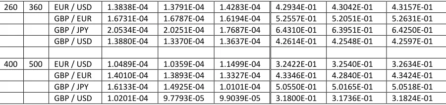
Table 6 Forecasting performance of one-day realized volatilities. This table reports the Root mean square error (RMSE) for the autoregressive neural network enhanced two-component model constructed by one hidden layer with 10 neurons (NNE2C 10 neurons), Component GARCH model, EGARCH model, and autoregressive neural network model constructed by one hidden layer with 10 neurons (NNOnly 10 neurons), for the forecasting interval 𝝉𝟏 to 𝝉𝟐, where 𝝉𝟏= 𝒎𝒂𝒙(𝟏, 𝝉𝟐− 𝟏𝟎𝟎), for the one-day realized volatilities of four currencies.

𝜏1 𝜏2 NNE2C

(10 neurons)

CGARCH EGARCH NNOnly

(10 neurons)

1 20 EUR / USD 1.7692E-04 5.4301E-04 1.7308E-03 5.7113E-01 GBP / EUR 1.3087E-04 2.1771E-04 7.0773E-04 4.3658E-01 GBP / JPY 2.2910E-04 1.5067E-05 1.3846E-04 7.7768E-01 GBP / USD 3.4074E-04 3.1626E-03 5.9010E-04 1.4300E+00

5. Conclusions

(24)

23 Therefore, we name the proposed model as “neural network enhanced two-component volatility model”. The model was thoroughly evaluated using high frequency tick data of four currencies across six forecasting horizons. The out-of-sample forecasting results consistently and significantly outperform the Component GARCH and EGARCH models as well as the autoregressive neural network model, which is applied on modelling the volatility directly.

The results reported in this paper are based on two simple structures: the low-pass Hodrick-Prescott filter uses a fixed smoothing parameter and the short-term component follows a first order autoregressive progress. Future work would be to consider using an optimized smoothing parameter that decomposes a stationary term component. A higher order ARMA process would provide a better fit for the decomposed short-term component and may bring improved out-of-sample forecasting performance. Moreover, a higher smoothing parameter brings more smoothed long-term component, which can be easier to forecasting by neural network with higher accuracy, and decomposes a more volatile short-term component, which may not follow a stationary process. Indeed, it would be a sufficiently further improvement if considering the forecasting model as an optimization framework to find an optimal parameter, which decomposes a stationary short-term process while maintaining a smooth long-term component, which can be forecasted by autoregressive neural network with high accuracy.

Acknowledgement

(25)

24

6. References

Alizadeh, S., Brandt, M. W., & Diebold, F. X. (2002). Range‐based estimation of stochastic volatility models. Journal of Finance, 1047-1091.

Aljarah, I., Faris, H., Mirjalili, S., & Al-Madi, N. (2016). Training radial basis function networks using biogeography-based optimizer. Neural Computing and Applications, 1-25.

Andersen, T., & Bollerslev, T. (1998). Answering the skeptics: Yes, standard volatility models do provide accurate forecasts. International economic review, 885-905.

Andreou, P. C., Charalambous, C., & Martzoukos, S. H. (2008). Pricing and trading European options by combining artificial neural networks and parametric models with implied parameters. European Journal of Operational Research, 1415–1433.

Baxter, M., & King, R. G. (1999). Measuring Business Cycles Approximate Band-Pass Filters for Economic Time Series. Review of Economics and Statistics, 575-593.

Bollerslev, T. (1990). Modelling the coherence in short-run nominal exchange rates: a multivariate generalized ARCH model. The review of economics and statistics, 498-505.

Boyacioglu, M. A., & Avci, D. (2010). An Adaptive Network-Based Fuzzy Inference System (ANFIS) for the prediction of stock market return: The case of the Istanbul Stock Exchange. Expert Systems with Applications, 7908–7912.

Brandt, M., & Jones, C. (2006). Volatility forecasting with range-based EGARCH models. Journal of Business and Economic Statistics, 61–74.

Charalambous, C. (June 1992). Conjugate gradient algorithm for efficient training of artificial neural networks. IEE Proceedings G - Circuits, Devices and Systems, 301 - 310.

Gorr, W. L. (June 1994). Research prospective on neural network forecasting. International Journal of Forecasting, 10(1), 1-4.

Granger, C. W. (1980). Long memory relationships and the aggregation of dynamic models. Journal of econometrics 14.2, 227-238.

Granger, C. W., & Joyeux, R. (1980). An introduction to long‐memory time series models and fractional differencing. Journal of time series analysis, 15-29.

Hagan, M. T., & Menhaj, M. B. (1994). Training feedforward networks with the Marquardt algorithm. IEEE transactions on Neural Networks, 989-993.

(26)

25 Harris, R. D., Stoja, E., & Yilmaz, F. (2015). A cyclical model of exchange rate volatility. Journal of Banking

& Finance, 3055-3064.

Hodrick, R. J., & Prescott, E. C. (1997). Postwar US business cycles: an empirical investigation. Journal of Money, credit, and Banking, 1-16.

Jesús, R. J. (2016). A method with neural networks for the classification of fruits and vegetables. Soft Computing, 1–14.

Jia, Z., Yi, C., Yuan, Y., Xuemei, D., & Yuhua, L. (2017). Coarse and fine identification of collusive clique in financial market. Expert Systems with Applications, 225–238.

Jiang, Y., Ahmed, S., & Liu, X. (2016). Volatility forecasting in the Chinese commodity futures market with intraday data. Review of Quantitative Finance and Accounting, 1-51.

Kristjanpoller, & Minutolo. (2016). Forecasting volatility of oil price using an artificial neural network-GARCH model. Expert Systems With Applications, 65, 233–241.

Kristjanpoller, W., Fadic, A., & Minutolo, M. (2014). Volatility forecast using hybrid Neural Network models. Expert Systems with Applications, 2437–2442.

Lee, G. G., & Engle, R. F. (1999). A Permanent and Transitory Component Model of Stock Return Volatility. In R. Engle, & H. White, Cointegration, Causality, and Forecasting: A Festschrift in Honor of Clive W. J. Granger (pp. 475-497). Oxford: Oxford: Oxford University Press.

Liu, Q., Yin, J., Leung, V. C., Zhai, J.-H., Cai, Z., & Lin, J. (2016). Applying a new localized generalization error model to design neural networks trained with extreme learning machine. Neural Computing and Applications, 59–66.

McDonald, S., Coleman, S., McGinnity, Li, Y., & Belatreche, A. (2014). A comparison of forecasting approaches for capital markets. 2104 IEEE Conference on Computational Intelligence for Financial Engineering & Economics (CIFEr). London: IEEE.

McDonald, S., Coleman, S., McGinnity, T. M., & Li, Y. (2013). A hybrid forecasting approach using ARIMA models and self-organising fuzzy neural networks for capital markets. The 2013 International Joint Conference on Neural Networks (IJCNN). Dallas: IEEE.

McElroy, T. (2008). Exact Formulas for the Hodrick-Prescott Filter. Econometrics Journal, 209–217. Mustafaraj, Lowry, & Chen. (2011). Prediction of room temperature and relative humidity by autoregressive

linear and nonlinear neural network models for an open office. Energy and Buildings, 1452–1460. Nelson, M., Hill, T., Remus, W., & O'Connor, M. (1999). Time series forecasting using NNs: Should the

(27)

26 Poon, S.-H., & Granger, C. W. (2003). Forecasting Volatility in Financial Markets: A Review. Journal of

Economic Literature, 41(2), 478-539.

Ravn, M. O., & Uhlig, H. (2002). On adjusting the Hodrick–Prescott filter for the frequency of observations. Review of Economics and Statistics, 371-375.

Restrepo, A. R., Manotas, D. F., & Lozano, C. A. (2016 ). Self-generation of electricity, assessment and optimization under the new support schemes in colombia. IEEE Latin America Transactions, 1308 - 1314.

Rubio. (2016). Least square neural network model of the crude oil blending process. Neural Networks, 88– 96.

Rubio, J. d., Elias, I., Cruz, D. R., & Pacheco, J. (2016). Uniform stable radial basis function neural network for the prediction in two mechatronic processes. Neurocomputing, 122–130.

Sharda, R., & Patil, R. B. (Oct 1992). Connectionist approach to time series prediction: an empirical test. Journal of Intelligent Manufacturing, 317–323.

Siegelmann, H., Horne, B., & Giles, C. (1997 ). Computational capabilities of recurrent NARX neural networks. IEEE Transactions on Systems, Man, and Cybernetics, Part B (Cybernetics), 208 - 215. Stock, J. H., & Watson, M. W. (1999). Forecasting Inflation. Journal of Monetary Economics, 293–335. Stock, J., & Watson, M. (2016). Dynamic Factor Models, Factor-Augmented Vector Autoregressions, and

Structural Vector Autoregressions in Macroeconomics. In J. B. Taylor, & H. Uhlig, Handbook of Macroeconomics (pp. Volume 2, 415–525). ELSEVIER.

Svalina, I., Galzina, V., Lujić, R., & Šimunović, G. (2013). An adaptive network-based fuzzy inference system (ANFIS) for the forecasting: The case of close price indices. Expert Systems with Applications, 6055–6063.

Tim, B. (1986). Generalized autoregressive conditional heteroskedasticity. Journal of econometrics 31.3, 307-327.

Torben, A., Tim, B., & Francis, D. (2009). Parametric and nonparametric measurements of volatility. In Y. Aït-Sahalia, & L. P. Hansen, Handbook of Financial Econometrics. Amsterdam: North-Holland. W, B. M., & S, J. C. (2006). Volatility forecasting with range-based EGARCH models. Journal of Business

& Economic Statistics, 470-486.

(28)

27 Yi, C., Yuhua, L., Sonya, C., Ammar, B., & Martin, M. (2015). Adaptive Hidden Markov Model With Anomaly States for Price Manipulation Detection. IEEE Transactions on Neural Networks and Learning Systems, 318 - 330.

Yule, G. U. (1927). On a Method of Investigating Periodicities in Disturbed Series, with Special Reference to Wolfer's Sunspot Numbers. Philosophical Transactions of the Royal Society, 267–298.

Zhai, J., Cao, Y., Yao, Y., Ding, X., & Li, Y. (2017). Computational intelligent hybrid model for detecting disruptive trading activity. Decision Support Systems, 26–41.

Zhang, G., & Qi, M. (16 January 2005). Neural network forecasting for seasonal and trend time series. European Journal of Operational Research, 501–514.