Simplified Optimization Routine for Tuning Robust
Fractional Order Controllers
Cristina I. Muresan
Department of Automation, Faculty of Automation and Computer Science, Technical, University of Cluj-Napoca, Romania Email: [email protected]
Received June, 2013
ABSTRACT
Fractional order controllers have been used intensively over the last decades in controlling different types of processes. The main methods for tuning such controllers are based on a frequency domain approach followed by optimization rou-tine, generally in the form of the Matlab fminsearch, but also evolving to more complex routines, such as the genetic algorithms. An alternative to these time consuming optimization routines, a simple graphical method has been proposed. However, these graphical methods are not suitable for all combinations of the imposed performance specifications. To preserve their simplicity, but also to make these graphical methods generally applicable, a modified graphical method using a very straightforward and simple optimization routine is proposed within the paper. Two case studies are pre-sented, for tuning fractional order PI and PD controllers.
Keywords: Fractional Order Controllers; Graphical Tuning; Simplified Optimization Routine
1. Introduction
Fractional order PIDs (FO-PIDs) have been employed in various engineering fields ranging applications in a wide variety of domains. The fractional order PID controller is in fact a generalization of the classical integer order PID. In the fractional order PID control algorithm, the error signal is integrated and differentiated to any order, rather than to an integer order as with the traditional PIDs. The fractional order PIDs have two supplementary parame-ters compared to the traditional PIDs. It is for this reason, that the fractional order PIDs have the potential to meet more design specifications than the traditional PIDs and hence to increase the performance and robustness of closed loop systems [1-4]. A couple of interesting meth- ods have been proposed for tuning such FO-PIDs with the great majority centered upon Matlab’s fminsearch or graphical approaches [1, 5-7]. The current trend nowa- days is directed to the latter methods, since they require less computational and time resources. Nevertheless, if no exact solution exists, the current graphical methods fail at the tuning of the FO-PID controller.
The purpose of this paper is to design an improved graphical method for tuning FO-PI and FO-PD control- lers, based upon an optimization routine that selects the best possible tuning option even in the case of no exact solution. For exemplification, two case studies are con-sidered. The first case study implies the design of FO-PI control for a simple first order process. The second case
study consists in the design of a FO-PD controller for a second order process with integrator effect. Simulation results in both case studies show that the fractional order controllers tuned using the proposed algorithm can meet all performance specifications. To exemplify the opti-mized graphical methods for tuning fractional order con-trollers, the first case study has no exact solution, while the second case study has an exact solution.
The paper is organized as follows. Section 2 contains the main contribution of the present paper, with a de-scription of the fractional order PI and PD optimized graphical tuning algorithms, while Section 3 presents the two case studies. The final section contains the conclud-ing remarks.
2. Optimization Routine for Tuning
Fractional Order Controllers
The transfer function of the fractional order PI (FO-PI) controller is given by:
( ) 1 i
FO PI p
k
H s k
s
(1)
while the transfer function for the fractional order PD (FO-PD) controller is given by:
( ) 1
FO PD p d
H s k k s
(2)
where kp, ki and kd are the proportional, integral and de-
order. If 1, then the FO-PI controller in (1) is re- duced to a traditional PI controller:
( ) 1 i
FO PI p
k
H s k
s
(3)
and the FO-PD is reduced to the classical PD controller by setting 1 in (2):
( ) 1
FO PD p d
H s k k s (4) A proper tuning of the FO-PI and FO-PD controllers in (1) and (3), as well as of the PI and PD controllers in (3) and (4), respectively, implies determining the values for the parameters, three in the case of the FO-PI and FO-PD controllers and two in the case of the traditional PI and PD controllers. For tuning FO-PI and FO-PD controllers, in order to uniquely determine the three parameters - , kp and ki in the case of the FO-PI and , kp and kd in the
case of the FO-PD– three equations are used that de- scribe the performance of the closed loop system. The general approach regarding the tuning of fractional order controllers is based on frequency domain performance specifications [8-10], which refer to imposing a gain crossover frequency, a phase margin and robustness to open loop gain variations.
For a general process transfer function Hp(s), the open
loop system when s j is written as:
( ) ( ) ( )
oop FO PI P
open l
H j H j H j (5)
where is the frequency.
In order for the open loop system to attain an imposed gain crossover frequency gc, then the following rela-
tion must hold:
( )
open loop gc
H j 1 (6)
where denotes the modulus of the complex function. The open loop phase margin, m, is also computed at
the gain crossover frequency as:
( )
open loop gc m
H j
(7)
where denotes the phase of the complex function. Finally, the last performance specification, robustness to gain variations, implies that the phase of the open loop system at the gain crossover frequency should be flat:
( )
0 open loop gc
gc
d H j
d
(8)
2.1. Optimization Routine for Tuning Fractional Order PI Controllers
The transfer function of the FO-PI controller, in the fre- quency domain, may be written as:
( )
PI
H j 1 cos sin
2 2
FO kp ki j
(9)
in which
1 1 cos sin
2 j 2
s j (10)
Equations (6), (7) and (8) imply a certain behavior of the closed loop system, according to the specified values for the gain crossover frequency and the phase margin, and may further be used to determine all three values for the kp, ki and parameters of the FO-PI controller:
1 cos sin 1 (
2 2 gc
p i gc p
k k j H j
) (11)
sin
2 ( )
cos 2 i
m p gc
gc i
k
tg H j
k (12) 1 2 2
sin ( )
2
1 2 cos
2 i gc
p gc
gc
i gc i gc
k d H j
d k k (13)
where Hp(s) is the process transfer function.
Using solely equations (12) and (13), ki and may
be determined uniquely, while (11) may be then used to determine kp. The simplest method for computing the
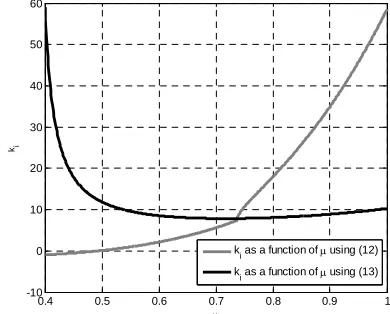
FO-PI parameter values is based on a graphical approach [1, 5-7], which implies that ki is computed and plotted as
a function of using equations (12) and (13). The in- tersection point of the resulting two curves yields the final values for ki and . Consequently, kpis
deter-mined using (11) and the previously graphically selected values for ki and . Such an example is given in
Fig-ure 1.
Although this method proves to be highly efficient and simple, the graphical approach is based upon the inter- section of the curves resulting from (12) and (12). Such
0.4 0.5 0.6 0.7 0.8 0.9 1 -10 0 10 20 30 40 50 60 ki
[image:2.595.324.519.545.702.2]ki as a function of using (12) ki as a function of using (13)
Figure 1. Selection of ki andaccording to the intersection
an intersection point depends upon the imposed criteria for the gain crossover frequency and the phase margin. For a specified set of gain crossover frequency and phase margin, such an intersection point might not exist. Thus, the existing graphical methods cannot be used to com- pute the parameters and optimization algorithms need to be used instead.
In order to facilitate the use of the simplicity of the graphical methods in tuning the FO-PI controllers and to avoid complex optimization algorithms, a simple approach is proposed that combines the graphical methods with a very simple optimization routine. The idea behind the optimization routine consist in plotting the two curves for
ki as a function of and selecting the values that
minimize the distance between the two plotted curves. The proposed tuning algorithm is given below:
for 0 :1
compute ki using (12)
store result in vector ki1
compute ki using (13)
store result in vector ki2
end
plot ki1 as a function of
plot ki2 as a function of
compute absolute value of distance = ki1-ki2
determine optim = min(distance) return optim corresponding to optim
compute ki using (13) and optim
compute kp using (11)
The algorithm for computing PI controllers is based upon setting 1 and computing ki using either (12) or
(13) and kp using (11). Since, the PI controller in (3) has
only two design parameters, the tuning of the PI control- ler may be done using any combination of two perform- ance criteria in (11), (12) or (13). Thus, imposing (11) and (12) means that (13) will not necessarily be ensured, which is the main drawback of traditional PI controllers as compared to FO-PI controllers.
2.2. Optimization Routine for Tuning Fractional Order PD Controllers
The tuning of the FO-PD controller is achieved in a similar manner to the FO-PI. The transfer function of the FO-PD controller, in the frequency domain, may be written as:
( ) 1 cos sin
2 2
FO PI p d
H j k k j
(14)
in which
cos sin2 2
s j j
(15)
Similar to the FO-PI situation, equations (6), (7) and (8)
may be used to determine the three parameters of the FO-PD controller, kp, kd and :
1
1 cos sin
2 2 ( gc)
p d gc
p
k k j
H j
(16)
sin
2 ( )
cos 2 d
m p gc
gc d
k
tg H j
k
(17)
1
2 2
sin ( )
2
1 2 cos
2
d gc p gc
gc
d gc d gc
k d H j
d
k k
(18)
Then, (17) and (18) may be employed to determine using the optimized graphical algorithm the parameters kd and , and then, kp may be computed directly using
(16), as described below: for 0:1
compute kd using (17)
store result in vector kd1
compute kd using (18)
store result in vector kd2
end
plot kd1 as a function of
plot kd2 as a function of
compute absolute value of distance = kd1-kd2
determine optim = min(distance) return optim corresponding to optim
compute kd using (18) and optim
compute kp using (16)
The algorithm for computing PD controllers is based upon setting 1 and computing kd using either (17)
or (18) and kp using (16). Since, the PD controller in (4)
has only two design parameters; the tuning of the PD controller may be done using any combination of two performance criteria in (16), (17) or (18). Thus, imposing (16) and (17) means that (18) will not necessarily be en- sured, which is the main drawback of traditional PD con- trollers as compared to FO-PD controllers.
3. Case Studies
3.1. Tuning an FO-PI Controller for a First Order Process
The process transfer function is given by: 27.5
( )
0.26 1
p H s
s
(19)
For a gain crossover frequency of cg =15 rad/s and
a phase margin of m=70o, the curves in Figure 1 are
ler parameters. Imposing slightly different performance criteria, such as cg=30 rad/s, m=70o and robustness
to gain uncertainties, the two curves in Figure 2 are ob- tained.
For these particular performance criteria, the two plots for ki do not intersect. Nevertheless, using the algorithm
proposed in Section 2, the minimum distance between the two curves is computed, yielding 0.55 and ki=
5.69. Finally, using (11) the remaining FO-PI parameter is computed as kp=0.1677.
The resulting (FO-PI) is:
0.55
5.69 (
PI
HFO s) 0.1677
s
1
[image:4.595.311.532.86.270.2] (20)
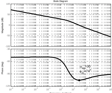
Figure 3 shows that the Bode plot of the open loop system with a FO-PI controller. It can be seen that the phase margin is slightly increased from 70o as imposed
to74o. This is due to the optimization algorithm, in which
the final value for ki is chosen in order to meet the ro-
bustness criteria, rather than the phase margin criteria. However, thanks to the optimal choice for the fractional order , the phase margin criteria obtained does not vary significantly from the one imposed in the design phase. The Bode plot also indicates that the modulus crosses the zero axes at 30rad/s, as imposed in the design specifications. Most importantly, it can be seen, that changing the open loop gain will not reduce the phase margin, but rather increase it, which means that the overshoot of the closed loop system will not vary sig- nificantly from the nominal value. Hence, the closed loop system should behave robustly despite uncertainties in the gain variations.
The closed loop results considering ±50% gain uncer- tainty are given in Figure 4. It can be seen that the FO-PI controller maintains the overshoot below 5%, while the settling time varies slightly between 0.15-0.25 seconds.
0.4 0.45 0.5 0.55 0.6 0.65 0.7 0.75 0.8 0
2 4 6 8 10 12
ki
ki as a function of using (12) ki as a function of using (13)
Figure 2. Plots of ki as a function of μusing (12) and (13) for
ωcg = 25 rad/s and φm = 70o
-100 -50 0 50 100
Mag
ni
tud
e (
d
B
)
Bode Diagram
Frequency (rad/sec)
10-4 10-3 10-2 10-1 100 101 102 103 104
-120 -90 -60 -30
P
has
e (
de
g)
cg=30 m=74o
Figure 3. Open loop Bode diagram using FO-PI controller.
0 0.1 0.2 0.3 0.4 0.5 0.6
0 0.2 0.4 0.6 0.8 1 1.2 1.4
Time (s)
Ou
tp
u
t
[image:4.595.311.536.305.492.2]+50% gain uncertainty -50% gain uncertainty nominal case
Figure 4. Closed loop results with FO-PI controller consid-ering ±50% process gain variation.
3.2. Tuning an FO-PD Controller for a Second Order Process
The process transfer function is given as:
1 ( )
( 0.5) p
H s s s
(21)
Taking ωcg = 15 and m = 50O and using the algorithm
described in Section 2, the plots of kd as a function of μ
are derived as given in Figure 5. In this case, the algo-rithm presented in Section 2 yields the same result as any of the existing graphical methods, since the two curves intersect. Figure 5 finally yields a fractional order λ= 0.573 and kd =2.59.
Using (16), the following value is obtained for the kp
[image:4.595.64.282.530.705.2]The resulting (FO-PD) is:
0.573
( ) 17.5 1 2.59 FO PD
H s s (22)
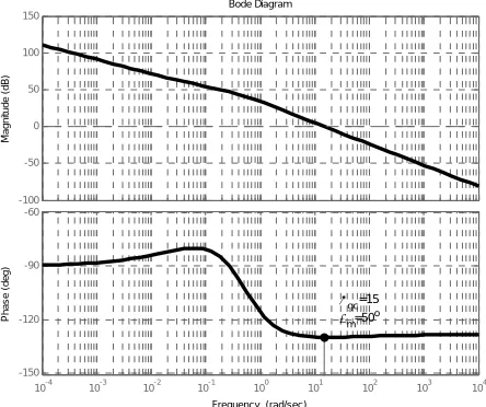
The Bode diagram of the open loop system using the previously determined FO-PD controller is given in Fig- ure 6, while the closed loop system considering ±50% gain uncertainty is given in Figure 7.
The Bode diagram in Figure 6 shows that variations of the open loop gain will not have a negative effect on the overshoot of the closed loop system, but only on the set-tling time, which demonstrates that the designed frac-tional order PD controller ensures the robustness of the closed loop system despite gain variations. As compared to the fractional order PI controller, the solution of the PD controller at the intersection of the two curves im-plies that all performance specifications are met: the gain crossover frequency is exactly 15 rad/sec, as specified, the phase margin is exactly 50o and the phase plot is flat
around the gain crossover frequency.
0.56 0.58 0.6 0.62 0.64 0.66 0.5
1 1.5 2 2.5 3 3.5 4 4.5 5 5.5
kd
kd as a function of using (17) k
[image:5.595.313.536.85.281.2]d as a function of using (18)
Figure 5. Selection of the fractional order μ and kd parameter.
-100 -50 0 50 100 150
Magni
tu
d
e
(
d
B
)
Bode Diagram
Frequency (rad/sec)
10-4 10-3 10-2 10-1 100 101 102 103 104
-150 -120 -90 -60
Ph
a
s
e
(
d
e
g
)
gc=15 m=50
o
Figure 6. Bode diagram of the open loop system with FO-PD controller.
0 0.2 0.4 0.6 0.8 1
0 0.2 0.4 0.6 0.8 1 1.2 1.4
Time (s)
O
ut
put
[image:5.595.64.282.326.488.2]+50% gain uncertainty -50% gain uncertainty nominal case
Figure 7. Closed loop responses considering ±50% gain uncertainty with a FO-PD controller.
As expected from the Bode plot, the overshoot is maintained in all three case scenarios at the value of 25%, while the settling time varies between 0.3-0.6 seconds.
4. Conclusions
The purpose of the present paper was to present a simple and efficient optimization algorithm for tuning fractional order PI and PD controllers. For specific performance criteria, the existing graphical methods may not yield an exact solution. Thus, optimization routines need to be used in order to tune the fractional order controllers. The paper shows that even in the case of no exact solution, the graphical methods may still be employed with a slight modification that implies computing and selecting the minimum distance between the possible solutions. It is shown through simulations that the fractional order controllers designed using the proposed method yield satisfactorily results in terms of closed loop performance and robustness.
5. Acknowledgements
This work was supported by a grant of the Romanian National Authority for Scientific Research, CNCS – UE- FISCDI, project number PN-II-RU-TE-2012-3-0307.
REFERENCES
[1] C.A. Monje, Y. Chen, B. M. Vinagre, D. Xue and V. Feliu, “Fractional-order Systems and Controls: Funda-mentals and Applications,” Springer, London, 2010. doi:10.1007/978-1-84996-335-0
[image:5.595.61.283.521.707.2]Video Processing, Vol. 6, 2012, pp. 453-461. doi:10.1007/s11760-012-0322-4
[3] A. Oustaloup,” La Commande CRONE: Commande Ro-bust d’ordre non entiere,” Hermes, Paris, France, 1991 [4] C. A. Monje, B. Vinagre, Y. Chen and V. Feliu, “On
Fractional PIλcontrollers: Some Tuning Rules for Ro-bustness to Plant Uncertainties,” Nonlinear Dynam, Vol. 38, 2004, pp. 369-381. doi:10.1007/s11071-004-3767-3 [5] C. I. Muresan, E. H. Dulf, R. Both, A. Palfi and M.
Ca-prioru, “Microcontroller Implementation of a Multivari-able Fractional Order PI Controller,” The 9th Interna-tional Conference on Control Systems and Computer Science (CSCS19-2013), 29-31 May, Bucharest, Romania, Vol. 1, 2013, pp. 44-51.
[6] Y. Luo and Y. Chen, “Fractional Order Motion Controls,” John Wiley & Sons, 2012.doi:10.1002/9781118387726
[7] Y. Luo, Y. Chen, C.Y. Wang and Y. G. Pi, “Tuning tional Order Proportional Integral Controllers for Frac-tional Order Systems,” Journal of Process Control, Vol. 20, 2010, pp. 823-831.
doi:10.1016/j.jprocont.2010.04.011
[8] C.A. Monje, B. Vinagre, Y. Chen and V. Feliu, “On Frac-tional PIλcontrollers: Some Tuning Rules for Robustness to Plant Uncertainties,” Nonlinear Dynam, Vol. 38, 2004, pp. 369-381.doi:10.1007/s11071-004-3767-3
[9] Y. Q. Chen and K. L. Moore, “Discretization Schemes for Fractional-order Differentiators and Integrators,” IEEE T. Circuits.-I., Vol. 49, 2002, pp. 363-367.