Munich Personal RePEc Archive
On the fixed-effects vector decomposition
Breusch, Trevor and Ward, Michael B. and Nguyen, Hoa and
Kompas, Tom
Australian National University
March 2010
Online at
https://mpra.ub.uni-muenchen.de/26767/
On the Fixed-Effects Vector Decomposition
Trevor Breusch Michael B. Ward
Hoa Nguyen Tom Kompas
Crawford School of Economics and Government The Australian National University
Canberra, ACT 0200, Australia
email: [email protected] (corresponding author)
Version: July, 2010.
On the Fixed-Effects Vector Decomposition
Abstract: This paper analyses the properties of the fixed-effects vector
decompo-sition estimator, an emerging and popular technique for estimating time-invariant variables in panel data models with group effects. This estimator was initially moti-vated on heuristic grounds, and advocated on the strength of favorable Monte Carlo results, but with no formal analysis. We show that the three-stage procedure of this decomposition is equivalent to a standard instrumental variables approach, for a specific set of instruments. The instrumental variables representation facilitates the present formal analysis which finds: (1) The estimator reproduces exactly classical fixed-effects estimates for time-varying variables. (2) The standard errors recom-mended for this estimator are too small for both time-varying and time-invariant variables. (3) The estimator is inconsistent when the time-invariant variables are endogenous. (4) The reported sampling properties in the original Monte Carlo evi-dence do not account for presence of a group effect. (5) The decomposition estimator has higher risk than existing shrinkage approaches, unless the endogeneity problem is known to be small or no relevant instruments exist.
1. INTRODUCTION
We analyse the properties of a recently introduced methodology for panel data, known as fixed-effects vector decomposition (fevd), which Pl¨umper and Troeger
(2007a) developed to produce improved estimates in cases where traditional panel data techniques have difficulty. Researchers in many fields seek to exploit the advan-tages of such panel data. Having repeated observations across time for each group in a panel allows one, under suitable assumptions, to control for unobserved hetero-geneity across the groups which might otherwise bias the estimates. Mundlak (1978) demonstrated that a generalized least squares approach to unobserved group effects, which treats them as random and potentially correlated with the regressor, gives rise to the traditional fixed-effects (fe) estimator. However, feis a blunt instrument for
controlling for correlation between observed and unobserved characteristics because it ignores any systematic average differences between groups. Thus any potential explanatory factors that are constant longitudinally (time-invariant) will be ignored by the fe estimator. Likewise, any explanatory variables that have little within
Hausman and Taylor (1981) had previously shown that a better estimator than
fe is available if some of the explanatory variables are known to be uncorrelated
with the unobserved group effect, thus described asexogenous explanatory variables. The Hausman-Taylor (ht) estimator is an instrumental variables (iv) procedure
that combines aspects of both fixed-effects and random-effects estimation. Given a sufficient number of exogenous regressors, the ht procedure allows time-invariant
variables to be kept in the model. It also provides more efficient estimates than fe
for the coefficients of the exogenous time-varying variables. The downside of the ht
estimator resides in specifying the exogeneity status for each of the time-varying and time-invariant variables in the model. In many practical applications such detailed specification is onerous.
Pl¨umper and Troeger introduced fevdas an alternative that seemed to be
supe-rior to htbecause it requires fewer explicit assumptions yet seemed to always have
more desirable sampling properties. Like the fe estimator, and unlike ht, fevd
does not require specifying the exogeneity status of the explanatory variables. Like the ht estimator, and unlike fe, the fevd procedure gives coefficient estimates for
time-invariant (and slowly-changing) variables as well as the time-varying variables. Pl¨umper and Troeger motivated the fevd procedure on heuristic grounds, and
ad-vocated it on the strength of favorable results in a Monte Carlo simulation study. In particular, the simulation indicated that fevdhas superior sampling properties for
time-invariant explanatory variables.
Although the fevd procedure comes out of the empirical political science
liter-ature, it is rapidly finding application in many other areas including social research and economics. At last count there were well over 200 references in Google Scholar to this emerging estimation methodology. Several empirical studies report standard errors forfevd-based estimates that are strikingly smaller than estimates based on
traditional methods. There is, however, little formal analysis of thefevd procedure
in this literature.
The present paper is a remedy to the lack of formal analysis. We demonstrate that thefevd coefficient estimator can be equivalently written as aniv estimator, which
serves to demystify the nature of the three-stagefevdprocedure and its relationship
with other estimators. As one immediate benefit, the iv representation allows us to
draw on a standard toolkit of results.
First, using the iv variance formula, we show that the fevd standard errors for
coefficients of both the time-varying and time-invariant variables are uniformly too small. In the case of the latter variables, the discrepancy in thefevdstandard errors
Second, using the moment-condition representation, we prove that the coefficients of the time-varying variables in fevd are exactly the same as in fe. This result is
apparent in many of the practical studies which list fe estimates beside fevd
esti-mates, but it is hardly mentioned in the existing analytical material. An immediate implication is thatfevdestimates, likefe, areinefficient if any of the time-varying
variables are exogenous.
Third, fevd usually produces lower variance estimates of time-invariant
coeffi-cients thanhtin small samples. However, it does so by including invalid instruments
that produce inconsistent estimates. So, even with massive quantities of data those
fevdestimates will deviate from the truth.
Further developments can also be made to the estimator, to exploit the ideas in
fevd while avoiding the problems of that procedure. The advantage of fevd will
be found in smaller samples where the large sample concept of consistency does not dominate. The Monte Carlo simulation studies by Pl¨umper and Troeger (2007a) and Mitze (2009) show a trade-off between bias and efficiency in which fevd often
appears to be better than either feor htunder quadratic loss.
We present Monte Carlo evidence that a standard shrinkage approach combines the desirable small sample properties of fevd with the desirable large sample
prop-erties of the ht estimator, so that it has superior risk to both fevd and ht over a
wide region of the parameter space.
In the next section we introduce the notation to be used and describe the three-stage fevd estimator. We summarize the connections between these stages in a
theorem, which we prove by comparing the various moment conditions. This ap-proach demonstrates naturally the description of thefevd estimator as iv. Section
3 compares the correct IV variance formula with the formula implicit in the stan-dard errors of the three-stage fevd approach. The main results are summarized in
2. THE MODEL
The data are ordered so that there areN groups each ofT observations. The model for a single scalar observation is
yit =Xitβ+Ziγ+ui+eit for i= 1, . . . , N and t= 1, . . . , T. (1)
Here, Xit is a k×1 vector of time-varying explanatory variables, and Zi is a p×1 vector of time-invariant explanatory variables.1 The parametersβ, γ, the group effect
ui, and the error termeitare all unobserved. Some elements ofXitorZiare correlated with the group effectui, in which case we call those variablesendogenous. Otherwise we call those variables exogenous. With endogenous explanatory variables standard linear regression techniques may produce estimates of the unknown parameters which are inconsistent in the sense that they do not converge to the true parameter values as the sample size grows large. One standard approach to this endogeneity problem is to use the instrumental variables technique developed by Hausman and Taylor.
Notation
The presentation is considerably simplified by introducing some projection matrix notation. Let
D=IN ⊗ιT, (2)
where IN is an N ×N identity matrix and ιT is a T ×1 vector of ones. That is, D
is a matrix of dummy variables indicating group membership. For any matrix M, we use PM = M(M′M)−1M′ to indicate the projection matrix for M, and we use
QM =I−PM to indicate the projection matrix for the nullspace of M. For example,
PD =D(D′D)−1D′ = 1
T(IN ⊗ιTι
′
T) (3)
is the matrix which projects a vector ontoD. This particular projection produces a vector of group means. That is,PDy={yi¯} ⊗ιT, where ¯yi = T1 PT
t=1yit. Also,
QD =IN T −PD (4)
is the matrix which produces the within-group variation. That is, QDy ={yit−yi¯}
is the NT ×1 vector of within-group differences.
1
The FEVD Estimator
The fevd proceeds in three stages, which we detail below. To sharpen the
analy-sis, we assume that the elements of Z are exactly time-invariant (not just slowly-changing), so thatPDZ =Z. An explicit analysis of the slowly-changing case yields qualitatively similar insights.
Stage 1 Perform a fixed effects regression of y on the time-varying X. The moment condition corresponding to a fixed effects regression is
(y−Xb)′QDX = 0. (5)
The unexplained component after this first step isy−Xb. The group-average of the unexplained component isPD(y−Xb).
Stage 2Regress the group-average of the unexplained component from the first step on the time-invariantZ. The moment condition is PD(y−Xb)−Zg′
Z = 0. Using the fact that PDZ =Z, this moment condition can be equivalently written as
(y−Xb−Zg)′Z = 0. (6)
The group-average residuals from this regression are
h=PD(y−Xb−Zg). (7)
Stage 3RegressyonX, Z, andh. The coefficients from this step are the final fevd
estimates. The moment conditions are
(y−Xβ−Zγ −hδ)′[X, Z, h] = 0. (8)
Theorem 1. The solution forβ isb from Stage 1; the solution for γ isg from Stage
2; and the solution for δ is one.
Proof. We need to verify that the moment conditions (8) are satisfied at β = b,
γ =g, andδ = 1. This requires that
(y−Xb−Zg−h)′[X, Z, h] = 0. (9)
Substituting in the definition ofh from (7) and gathering terms, this simplifies to
Using the fact that QDZ = 0, this further simplifies to
(y−Xb)′QD[X, Z, h] = 0. (11)
The first set of equalities in (11) must be satisfied, since it is identical to the moment condition (5) that defines b. The second set of equalities must be satisfied since
QDZ = 0. Similarly, the third set of equalities must be satisfied since QDh = 0, which follows from the definition ofh in (7) and the fact that QDPD = 0.
Instrumental Variables Representation
Using Theorem 1 we can show that thefevdestimator can also be expressed as an iv estimator for a particular set of instruments. The major benefit of using the iv
representation is that one can draw on a standard toolkit of results. Theorem 1 shows that the fevd estimates of β are identical to the standard fixed effects estimator b
from Stage 1. This estimator is defined by the moment condition (5). Theorem 1 also shows that the fevd estimates of γ are equivalent to the estimator of g from
Stage 2. This estimator is defined by the moment condition (6). Combining both moment conditions, and using the fact that QDZ = 0, the full moment conditions for the fevdestimator are
(y−Xβ−Zγ)′[QDX, Z] = 0. (12)
In other words, thefevdestimator is equivalent to aniv estimator using the
instru-ments QDX and Z.
3. VARIANCE FORMULAE
Using standard results forivestimators, the asymptotically correct sampling variance
of the fevd procedure is
Viv(β, γ) = (H′W)−1H′ΩH(W′H)−1 for H = [QDX, Z] and W = [X, Z]. (13)
Here, H is the matrix of instruments and W is the matrix of explanatory variables. Ω is the covariance of the residual,ui+eit, which can be expressed as
Ω =σe2IN T +σu2IN ⊗ιTι′
T =σ
2
eQD + (σ
2
e +T σ
2
u)PD. (14)
We now compare the correctivvariance formula with thefevdvariance formula.
Pl¨umper and Troeger state that the sampling variance of thefevdestimator can be
obtained by applying the standardolsformula to the Stage 3 regression. Therefore,
Vfevd(β, γ, δ) =s2 [X, Z, h]′[X, Z, h]−1
=s2
X′X X′Z X′h
Z′X Z′Z Z′h
h′X h′Z h′h
−1
. (15)
Here, s2 = ky −Xβ −Zγ −hk2/dof, where dof is the degrees of freedom. By
application of (7), the expression fors2 can be simplified to
s2 =kQD(y−Xβ)k2/dof, (16)
which we note is the standard textbookfeestimator forσe2 whendof =NT−N−k
(see e.g. Wooldridge, 2002, p. 271).2
Now consider the variance of β. The fevd variance formula for β is the
top-left block of the overall fevdvariance formula in (15); using the partitioned-inverse
formula this submatrix can be written as
Vfevd(β) = s2(X′Q
[Z,h]X)−1. (17)
By expanding out (13), the correct variance forβ can be written as
Viv(β) = σ2e(X′QDX)−1. (18)
Note that this is exactly the textbook fixed effects variance formula. Now we note from (16) that s2 is a consistent estimator of σ2
e. However, the
matrices in the fevd formula (17) and the correct formula (18) differ. The fevd
variance formula forβ must therefore be incorrect, and we can show the direction of the error.
Theorem 2. The fevd variance formula for coefficients on time-varying variables
is too small.
2
The usualolsformula for the standard errors from the Stage 3 regression would calculate the
scale term usingdof =N T−k−p−1, wherepis the number ofZvariables including the constant and the final minus one allows for the additional regressorh. This divisor would clearly produce an inconsistent estimator ofσ2
e for large N and small T. Pl¨umper and Troeger (2007a, p. 129)
mention briefly an adjustment to the degrees of freedom and, although they do not give an explicit formula, their software employs the divisor dof = N T −N −k−p+ 1 (Pl¨umper and Troeger, 2007b). This adjustment would yield a consistent estimate ofσ2
e, but it is nonstandard and slightly
biased. To sharpen the subsequent analysis, we use the standard unbiased estimator ofσ2
e, in which
Proof. Now PD[Z, h] = [Z, h], so that PDP[Z,h]=P[Z,h]. Such a relationship between
projection matrices implies thatPD−P[Z,h]is positive semi-definite (in matrix
short-hand, PD ≥ P[Z,h]). So, QD ≤ Q[Z,h]. That (X′Q[Z,h]X)−1 ≤ (X′QDX)−1 follows
immediately. This inequality will almost always be strict because thep+ 1 variables [Z, h] cannot span the whole of the N-dimensional space of group operatorD, and the X’s have arbitrary within-group variation.
The fevdformula for the variance ofβ is biased in that it systematically
under-states the true sampling variance of the estimator. The essential inequality does not disappear as N gets larger, so the formula is also inconsistent. The usual reported standard errors will be too small.
Now, consider the variance of γ. The fevd variance formula for γ is the middle
block of the overall fevd variance formula in (15). Using an alternative
representa-tion of the partirepresenta-tioned inverse, this submatrix can be written as
Vfevd(γ) = s2(Z′Z)−1I+Z′[X, h] [X, h]QZ[X, h]−1
[X, h]′Z(Z′Z)−1. (19)
Note thatZ′h= 0, so that in the partitioned central matrix of the second term only the submatrix corresponding toX will be selected. Then, we have the simplification of (19),
Vfevd(γ) = s2(Z′Z)−1+s2(Z′Z)−1Z′X X′QZX−1
X′Z(Z′Z)−1. (20)
In contrast, by expanding out (13), the correct variance for γ can be written as
Viv(γ) =σ2e(Z′Z)−1+T σ2
u(Z′Z)−
1+σ2
e(Z′Z)−
1Z′X(X′QDX)−1X′Z(Z′Z)−1. (21)
Again, s2 is a consistent estimator of σ2
e, so the first term in (20) and in (21) is
essentially the same. However, the expressions are otherwise different, so the fevd
variance formula for γ must also be incorrect. Again, we can show the direction of the error.
Theorem 3. The fevd variance formula for time-invariant variables is too small.
Proof. As shown in the proof of Theorem 2, (X′QDX)−1 ≥ (X′Q
[Z,h]X)−1 with
almost certain strict inequality, so the last term in the fevd variance formula (20)
understates the corresponding term in the correct variance expression (21). The only exception would be the unlikely event that X and Z are exactly orthogonal, causing those terms to vanish. But even then, the fevd variance formula will be
an understatement because it omits the term T σ2
u(Z′Z)−1, which must be positive
In general the fevd variance formula for γ is systematically biased and
incon-sistent. The usual reported standard errors will be too small. The extent of the downward bias is unbounded. The correct variance expression includes a term that is directly proportional to the number of observations per group T and to the vari-ance of the group effects σ2
u. In contrast thefevd variance formula, and hence the
standard errors, are unaffected by these parameters. By increasing either or both of these parameters, with everything else held constant, the extent of the downward bias in the fevdvariance formula becomes arbitrarily large.
Empirical Example
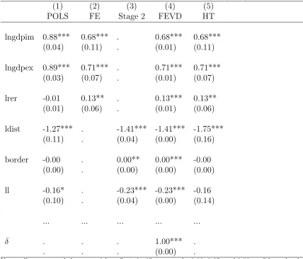
Reported results from the applied empirical literature align with these theoretical results. Table 1 presents our replication of Table 1 in Belke and Spies (2008), and shows results for pooled ols (pols), fe, fevd, and ht. We add a column for the
results from Stage 2 of fevdand a row for the coefficient δthat arises in Stage 3 to
further illustrate our theoretical results.3 The first six variables only are shown for
brevity. They include logged nominal GDP of the importing country lngdim, logged nominal GDP of the exporting country lngdpex and logged bilateral real exchange rate lrer, as time-varying variables. The time-invariant variables shown are logged great circle distance in km ldist, border length in km border, and dummy for one or both countries being landlocked ll. Results are estimated from a panel sample of
N = 420 trading pairs for T = 14 years giving 5262 observations.
The coefficients for the first three (time-varying) variables are the same for fe
andfevd, as shown by Theorem 1. To illustrate the second aspect of Theorem 1, the
coefficients for the next three (time-invariant) variables are exactly equal in Stage 2 and FEVD, and the solution for δ is one. Theorem 2 is illustrated by the way the first three fevdreported standard errors are systematically smaller than the fe
ones, in an order of 0.01, 0.01 and 0.01, against 0.11, 0.07 and 0.06, even though the coefficients themselves are identical and the standard error formula forfeis well
established as being correct under the assumptions of the model.
It is a little harder to illustrate Theorem 3, which says that the fevd standard
errors on the time-invariant variables are similarly understated. However the ht
estimator is just-indentified in this case, which is the reason the ht coefficients
and standard errors for time-varying variables are exactly the same as fe. It is no
surprise, then, that the coefficient estimates of three time-invariant variables (which
3
Table 1: Partial replication of Belke and Spies (2008).
(1) (2) (3) (4) (5)
POLS FE Stage 2 FEVD HT
lngdpim 0.88*** 0.68*** . 0.68*** 0.68***
(0.04) (0.11) . (0.01) (0.11)
lngdpex 0.89*** 0.71*** . 0.71*** 0.71***
(0.03) (0.07) . (0.01) (0.07)
lrer -0.01 0.13** . 0.13*** 0.13**
(0.01) (0.06) . (0.01) (0.06)
ldist -1.27*** . -1.41*** -1.41*** -1.75***
(0.11) . (0.04) (0.00) (0.16)
border -0.00 . 0.00** 0.00*** -0.00
(0.00) . (0.00) (0.00) (0.00)
ll -0.16* . -0.23*** -0.23*** -0.16
(0.10) . (0.04) (0.00) (0.14)
... ... ... ... ...
δ . . . 1.00*** .
. . . (0.00) .
Notes: One, two, and three asterisks reflect significance at the 0.10, 0.05, and 0.01 confidence levels, respectively. Robust standard errors are in parentheses.
are all exogenous) are generally similar for pols, fevd, and ht. As expected, the htstandard errors are slightly larger but very close to those forpols, in an order of
0.16, 0.00 and 0.14 against 0.11, 0.00 and 0.10. However the fevd standard errors
are very small, at 0.00 in every case for the precision that is shown. This is most implausible, because one would not expect pols to be generally less efficient, given
the structure of this example.
both fe and fevd results (e.g. Caporale et al., 2009; Mitze, 2009; Krogstrup and
W¨alti, 2008). In the studies we examined, thefet-statistics were consistently smaller
than those reported for fevd time-varying variables — and often much smaller —
except for few cases affected by robust standard error formulae. Again, this is despite the fact that the coefficient estimators were actually identical by construction.
4. COMPARISON TO ALTERNATIVE ESTIMATORS
Thefevdestimator was introduced as an alternative to thehtinstrumental variable
estimator. By also expressing fevd in its instrumental variable representation we
are able to develop insights into their comparative properties. Hausman and Taylor showed that the standard fixed effects estimator is equivalent to anivestimator with
instrument set QDX. To that, they add any exogenous elements of X or of Z as further instruments.4
To see the relationship more clearly, decompose X and Z into exogenous and potentially endogenous sets: X = [X1, X2] and Z = [Z1, Z2], where the subscript 1
indicates exogenous variables and the subscript 2 indicates endogenous variables. The
ht procedure is then an iv estimator which uses the instrument set [QDX, X1, Z1].
In contrast, the fevd procedure is an iv estimator which uses the instrument set
[QDX, Z1, Z2].
The first essential difference between these estimators is that thefevdinstrument
set excludes the exogenous time-varying variables X1. Of course, X1 may have no
members. In that case, the ht estimator for endogenous Z is not identified, so no
useful comparisons can be made.5 However, ifX
1 has known members, then a more
efficient estimator than fevd could be created by augmenting the instrument set
with X1. The second essential difference is that the fevd instrument set includes
the potentially endogenous time-invariant variablesZ2. If these variables are in fact
correlated with the group effect, then thefevd estimator is inconsistent.
The fevdand ht estimators coincide exactly when there are no exogenous
ele-ments ofXand no endogenous elements ofZ.6 Thefevdprocedure is thus primarily
of interest when someZ may in fact be endogenous. The essential question raised by
4
Hausman and Taylor describePDX as the additional instrument, but this interpretation follows
Breusch et al. (1989).
5
Ideally, one would have theoretical grounds for identifying which elements ofX are exogenous. As a practical matter, one could also use an over-identification test to confirm this assumption, since the fixed effects estimator ofβ is consistent.
6
Pl¨umper and Troeger is then whether it is better to use a biased and inconsistent but lower-variance estimator, or a consistent but higher-variance estimator. The ques-tion of whether a weak-instruments cure is worse than the disease is a sound one, which has been considered in other contexts by a variety of authors; see for example Bound et al. (1995).
Under a mean-squared error (mse) loss function, neither the fevd procedure
nor the ht procedure will uniformly dominate the other. mse can be expressed as
variance plus bias squared. Thus, a consistent estimator such ashtwill be preferable
to thefevdfor sufficiently large sample size.7 In contrast, for a small sample with a
small endogeneity problem, it might be preferable to include the the time-invariant endogenous variablesZ2 as instruments, as fevddoes. A more efficient estimator of
this type than fevd would be the iv estimator which augments the set of all valid
instruments with Z2, forming the instrument set [QDX, X1, Z].
One conventional approach to finding a balance would be to select between the competing estimators based on a specification test (Baltagi et al., 2003). If the test rejects the null hypothesis of no difference between estimators, then ht would be
selected. Otherwise, the efficient estimator estimator would be selected because the evidence of endogeneity is too weak. Selection of a final estimator based on the results of a preliminary test is known as a pretest procedure. Inference based on the standard errors of the final selected estimator alone may be misleading; however, bootstrap techniques which include the model selection step can circumvent this problem (Wong, 1997).
Since the work of James and Stein (1961), statisticians have understood that shrinking (biasing) an estimator toward a low-variance target can lower themse. An
extensive literature suggests shrinkage approaches based on using a weighted aver-age of two estimators when one estimator is efficient and the other is consistent; see for example Sawa (1973), Feldstein (1974), Mundlak (1978), Green and Strawder-man (1991), Judge and Mittelhammer (2004), or Mittelhammer and Judge (2005). We consider a shrinkage estimator which combines the consistent but inefficient ht
estimator and the efficient but possible inconsistent iv estimator. For purposes of
illustration, we choose a particularly simple shrinkage approach, but the literature contains many variations on the basic theme, which will have different strengths and weaknesses. If the bias, variance, and covariance of two estimators are known, it is algebraically straightforward to find the weight which minimizes the mse of a
combined estimator. In particular, suppose one estimator φ is unbiased. The other estimator χ is biased, but has lower variance. The shrinkage estimator then has the form χ+w(φ−χ), where w is the weight placed on the consistent estimator.
7
Straightforward calculus shows that optimal weight which minimizes mse is
w= µ
2
χ+σχ2 −σχφ µ2
χ+σ2χ+σφ2−2σχφ
, (22)
where bias is indicated by µand where variance is indicated by σ.
Of course, the exact bias and variances will usually not be known; however, prac-tical estimates of these terms are readily available foriv estimators. Mittelhammer
and Judge (2005) show that plugging in such empirical estimates produces a prac-tical weighted-average estimator. They choose a single w to minimize the sum of
mse over all coefficients. Since we are primarily interested in the mse of a single
coefficient in this analysis, we apply the solution for w, as presented in (22) which is the single-covariate case of equation 3.5 of Mittelhammer and Judge. We use standard empirical estimates of the variance and covariance terms from application of the basic iv formula (13). The difference between the two estimators provides
our estimate of the bias of the efficient estimator, since ht is asymptotically
unbi-ased. Mittelhammer and Judge provide detailed discussion on calculating bootstrap percentiles and standard errors, through application of Efron’s bias-corrected and accelerated bootstrap (Efron, 1987). The only change needed for the present context is to account for the panel structure, which is most simply done by resampling at the group level rather than resampling single observations independently.
5. MONTE CARLO EVIDENCE
In this section we compare the practical performance under a range of conditions of various estimators for an endogenous time-invariant Z. In addition to the fevd
and ht estimators, we consider a pretest estimator and a shrinkage estimator. The
pretest estimator selects between ht and the iv estimator based on the instrument
set set [QDX, X1, Z], which treats allZ as exogenous (asfevd does) in addition to
using the ht instruments. The pretest selection is based on the 95% critical value
of the Durbin-Wu-Hausman specification test for exogeneity ofZ (see e.g.Davidson and MacKinnon, 1993, p. 237). The shrinkage estimator assigns weights for the two estimators according to a first-stage empirical estimate of formula (22).
Pl¨umper and Troeger argue for the superiority of the fevd procedure over the ht approach based on Monte Carlo evidence. While our simulation design stays
close to the original design where appropriate, our design differ from theirs in two fundamental respects.8 The first difference is that in the Pl¨umper and Troeger Monte
8
Carlo study, thehtestimator was not actually consistent. This is because their data
generating process had no correlation between X and Z. The fact that the available instruments had, by construction, zero explanatory power for the endogenous variable contrasts sharply with their characterization of the Monte Carlo results (p. 130): “the advantages of thefevdestimator over the Hausman-Taylor cannot be explained
by the poor quality of the instruments.” Pl¨umper and Troeger note (in footnote 11) that the advantage of fevd persists in their experiments regardless of sample size.
However, the asymptotic bias of anivestimator is the same as the bias of olswhen
the instruments are uncorrelated with the endogenous variable, and thus irrelevant (Han and Schmidt, 2001). In contrast, with a valid and relevant instrument, the bias of the iv estimator will approach zero asymptotically. We therefore consider
scenarios in our simulation where the htestimator is consistent, that is at where at
least one instrument for the endogenous Z is valid and relevant.
The second difference is that our simulations account for random variation in the group effect, while the Pl¨umper and Troeger code holds the effect (u) fixed across all replications. Mundlak (1978) shows there is no loss of generality in assuming the effect is random, because the fixed-effects estimator and its related procedures can be described as inference conditional on the realizations of the effect in the sample. Further, the effect needs to be at least potentially random if the relationship between the effect and the regressors is to be described as correlation. As Mundlak shows, if the random effect is correlated with the group-averages of regressors in unknown ways, then the optimal linear estimator in the random-effects model is in fact the fixed-effectsestimator.
The code used by Pl¨umper and Troeger does not simply fix the replicated effects at some sample realization, rather it uses the Stata command ‘corr2data’ to fix the sample moments of the variables and the group effects exactly in every replication. The vector of effects is thereby ‘fixed’ by making it exactly orthogonal to the ex-ogenous variables, effectively excluding any practical influence of the group effect in the simulated data. That process does not simulate a fixed-effects model, but rather one in which there is no group effect at all! By contrast, our random-effects simulation represents the situation where the analyst is uncertain of the magnitudes of the group effects.
We run a series of experiments which vary the degree of endogeneity and strength of instrument. The data generating process for our simulation is
yit = 1 + 0.5x1+ 2x2−1.5x3−2.5z1+ 1.8z2+ 3z3+ui+eit. (23)
Here, [x1, x2, x3] is a time-varying mean-zero orthonormal design matrix, fixed across
fixed across all experiments. z3 is fixed for all replications in each experiment. z3
has sample mean zero and variance 1, and is orthogonal to all other variables except
x1. The sample covariance of the group mean of x1 with z3 is set exactly to an
experiment-specific level, which allows us to vary the strength of the instrument across experiments.9 The idiosyncratic error termeis standard normal. The random
effect u is drawn from a normal distribution in each replication. The expectation of u conditional on z3 is ρz3, where ρ works out to be the value of cov(z3, u) set
in the experimental design. All other variables are uncorrelated with u, and the variance of u conditional on all variables is 1.10 The level of endogeneity is varied
across experiments by changing the value of cov(z3, u). Each experiment has 1000
replications, which vary the random components u and e. There are 30 groups (N) and 20 periods (T), as reported in Pl¨umper and Troeger (2007a). In implementing the estimators [x1, x2, z1, z2] are treated as known exogenous, while [x3, z3] are treated
as potentially endogenous.
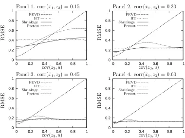
Figure 1 illustrates the simulation results for varying instrument strengths and endogeneity levels. The vertical axis in each panel is the square root of mse of
various estimators for the endogenous time-invariant variable z3. The horizontal
axis of each panel is the covariance between the random effectu and z3. Each panel
illustrates different instrument strength, as indicated by stronger instruments having higher correlation between the group-means of x1 and the endogenous variable z3.
The four panels display the experiments for corr(¯x1, z3) = 0.15,0.30,0.45, and 0.60
respectively.11 Note that, within each panel, the ht results are unchanging as a
consequence of the experimental design. Also, across panels, the fevd results are
unchanging by design.
The most notable feature of Figure 1 is that neither ht nor fevd uniformly
dominates the other. If reasonably strong instruments are available to implement the ht procedure, and endogeneity is an issue, htcan greatly outperform fevd as
shown in Panel 4 because the higher variance of htis compensated by lower bias.12
For all cases when endogeneity is absent (or is mild), fevdwill be the most efficient
estimator, as shown at the far left of all panels, because fevd exploits the true (or
9
Conditional on a non-zero sample correlation of the endogenous variable and the instrument, the moments of theivestimator exist, so the Monte Carlomseis well-defined.
10
The specified pattern of covariance is implemented through a Choleski decomposition approach.
11
Because variances of ¯x1 andz3 are both 1, the covariance of these variables equals their
corre-lation.
12
The discussion here focuses on the small sample properties. When N is very large, ht will
always outperform fevd if there is endogeneity and valid and relevant instruments exist. For a
Figure 1: Performance of the four estimators for varying instrument strengths 0 0.2 0.4 0.6 0.8 1 1.2 1.4
0 0.2 0.4 0.6 0.8 1
0 0.2 0.4 0.6 0.8 1 1.2 1.4
0 0.2 0.4 0.6 0.8 1
0 0.2 0.4 0.6 0.8 1 1.2 1.4
0 0.2 0.4 0.6 0.8 1 0
0.2 0.4 0.6 0.8 1 1.2 1.4
0 0.2 0.4 0.6 0.8 1
HT HT HT HT FEVD FEVD FEVD FEVD Shrinkage Shrinkage Shrinkage Shrinkage Pretest Pretest Pretest Pretest R M S E R M S E R M S E R M S E
cov(z3, u)
cov(z3, u)
cov(z3, u)
cov(z3, u)
Panel 1. corr(¯x1, z3) = 0.15 Panel 2. corr(¯x1, z3) = 0.30
Panel 3. corr(¯x1, z3) = 0.45 Panel 4. corr(¯x1, z3) = 0.60
approximately true) restriction thatz3 is uncorrelated withu. If the investigator has
strong prior reason to believe that endogeneity is not an issue, it makes sense to use that information. Indeed, with informative priors over endogeneity, using a Bayesian procedure which minimizes risk against that prior would be the ideal approach. However, usually, the investigator will be usingfe, orht, orfevdprecisely because
of concern that endogeneity might be a significant problem.
Rather than relying solely on prior information about the degree of endogeneity, the investigator can rely on evidence from within the dataset. Both the shrinkage and the pretest estimators are in this spirit. The shrinkage estimator in particular exhibits remarkably good risk characteristics across all ranges of all four panels, and it clearly dominates the pretest approach undermseloss. Indeed the shrinkage estimator often
has anmselower thanboth htandfevd, and never is much worse than the better of
problem is quite small.13 More generally, if incomplete or uncertain prior information
is available, alternatives which explicitly model that information, such as traditional Bayesian techniques or recent variants such as Bayesian model averaging (Hoeting et al., 1999), will likely be the best approach.
6. CONCLUSIONS
The fevd estimator of Pl¨umper and Troeger (2007a) offers the analyst of panel
data a way to include time-invariant (and slowly-changing) variables in the presence of group effects that are possibly correlated with the explanatory variables. Thus it appears superior to the existing leading approaches of fixed-effects (which omits the time-invariant variables) and Hausman-Taylor (which requires specifying the exogeneity status of each explanatory variable). Pl¨umper and Troeger’s motivation for the procedure was mostly heuristic and their evidence came from Monte Carlo experiments showing thatfevdoften displays better mean-squared error properties
than both fe and ht. The procedure can be implemented in three easy stages,
or even more conveniently in the Stata package provided by Pl¨umper and Troeger (2007b). This procedure has proved popular with panel data analysts.
Our analytical results and revised Monte Carlo experiments challenge the value of fevd. Is it still a useful tool?
We find that the coefficients of all the time-varying variables after the three stages of fevdare exactly the same as fein the first stage. This fact is sometimes seen in
the empirical applications but rarely commented upon with any clarity. Obviously, there is no gain in usingfevdover the simpler feif these coefficients are the objects
of interest. Further, if something is known about the exogeneity of explanatory vari-ables then these estimates are inefficient because they ignore the extra information. What is worse, unlike the simple first-stage fe, the standard errors from fevd are
too small — sometimes very much too small, judging from our empirical example and other published applications. In this case fevdis a definite step backwards.
The main attraction of fevdis its ability to estimate coefficients of time-invariant
explanatory variables. But, again the third stage is questionable. The same coef-ficient estimates are given in the second stage, which is a simple regression of the group-averaged residuals from fe on the time-invariant variables. The purported
13
While our focus is on estimator performance, it is worth noting that the Monte Carlo results do confirm that the asymptotic variance formula in (13) provides unbiased estimates of the ht
andfevdsampling variance, when σ2
e andσ
2
u are calculated with appropriate degrees of freedom
value of the third stage is to correct the standard errors, but this reasoning is now known to be false. Indeed there will be cases where the second-stage standard errors — even though they are known to be wrong — will be more accurate than those from the third stage. The example we have provided in Section 3 shows this possibility.
So if fevdis the label to describe the three-stage procedure, it cannot be
recom-mended for making inferences about any of the coefficients. The coefficient estimator, however, also represents a particular choice of instruments in standardiv. Dropping
the three-stage methodology and reverting to an explicit iv approach would allow
correct standard errors to be obtained in the cases where the estimator is consistent. However, since all of the time-invariant variables are used as instruments, the fevd
estimator will be inconsistent if any of these are endogenous. The value of this es-timator relative to others then depends on the trade-off between inconsistency and inefficiency.
When the objective is reduced mean-squared error, the literature is replete with other methods such as shrinkage estimators known to have good properties. We have provided one such estimator that clearly dominates the fevd estimator over
much of the parameter space and also limits the risk in regions where the fevd
risk is unbounded. In undertaking these investigations we have also uncovered an explanation for the misleading evidence favouring fevd that was suggested in the
REFERENCES
Baltagi, Badi H., Georges Bresson, and Alain Pirotte. 2003. Fixed effects, random effects or Hausman–Taylor? A pretest estimator. Economics Letters 79(3), 361– 369.
Belke, Ansgar and Julia Spies. 2008. Enlarging the EMU to the east: What effects on trade? Empirica 35(4), 369–89.
Bound, John., David A. Jaeger, and Regina M. Baker. 1995. Problems with in-strumental variables estimation when the correlation between the instruments and the endogenous explanatory variable is weak. Journal of the American Statistical Association 90(430), 443–50.
Breusch, Trevor S., Grayham E. Mizon, and Peter Schmidt. 1989. Efficient estimation using panel data. Econometrica 57(3), 695–700.
Caporale, Guglielmo M., Christophe Rault, Robert Sova, and Anamaria Sova. 2009. On the bilateral trade effects of free trade agreements between the EU-15 and the CEEC-4 countries. Review of World Economics 145(2), 189–206.
Davidson, Russell and James G. MacKinnon. 1993. Estimation and Inference in Econometrics. Oxford University Press.
Efron, Bradley. 1987. Better bootstrap confidence intervals. Journal of the American Statistical Association 82(397), 171–85.
Feldstein, Martin. 1974. Errors in variables: A consistent estimator with smaller MSE in finite samples. Journal of the American Statistical Association 69(348), 990–96.
Green, Edwin J. and William E. Strawderman. 1991. A James-Stein type estimator for combining unbiased and possibly biased estimators. Journal of the American Statistical Association 86(416), 1001–06.
Han, Chirok and Peter Schmidt. 2001. The asymptotic distribution of the instrumen-tal variable estimators when the instruments are not correlated with the regressors.
Economics Letters 74(1), 61–66.
Hoeting, Jennifer A., David Madigan, Adrian E. Raftery, and Chris T. Volinsky. 1999. Bayesian model averaging: A tutorial. Statistical Science 14(4), 382–401.
James, W. and Charles Stein. 1961. Estimation with quadratic loss. In J. Neyman (Ed.), Proceedings of the Fourth Berkeley Symposium on Mathematical Statistics and Probability, Volume 1, pp. 361–79. University of California Press.
Judge, George G. and Ron C. Mittelhammer. 2004. A semiparametric basis for combining estimation problems under quadratic loss. Journal of the American Statistical Association 99(466), 479–87.
Krogstrup, Signe and S´ebastien W¨alti. 2008. Do fiscal rules cause budgetary out-comes? Public Choice 136(1), 123–138.
Mittelhammer, Ron C. and George G. Judge. 2005. Combining estimators to im-prove structural model estimation and inference under quadratic loss. Journal of Econometrics 128(1), 1–29.
Mitze, Timo. 2009. Endogeneity in panel data models with varying and time-fixed regressors: to IV or not IV? Ruhr Economic Paper No. 83.
Mundlak, Yair. 1978. On the pooling of time series and cross section data. Econo-metrica 46(1), 69–85.
Pl¨umper, Thomas and Vera E. Troeger. 2007a. Efficient estimation of time-invariant and rarely changing variables in finite sample panel analyses with unit fixed effects.
Political Analysis 15(2), 124–39.
Pl¨umper, Thomas and Vera E. Troeger. 2007b. xtfevd.ado version 2.00 beta. Accessed from http://www.polsci.org/pluemper/xtfevd.ado.
Sawa, Takamitsu. 1973. The mean square error of a combined estimator and numer-ical comparison with the TSLS estimator. Journal of Econometrics 1(2), 115–32.
Wong, Ka-fu. 1997. Effects on inference of pretesting the exogeneity of a regressor.
Economics Letters 56(3), 267–71.
APPENDIX
[image:23.612.110.490.213.496.2]Monte Carlo results for large N and small T.
Figure 2: Relative estimator performance whenN = 300 and T = 2
0 0.2 0.4 0.6 0.8 1
0 0.2 0.4 0.6 0.8 1
0 0.2 0.4 0.6 0.8 1
0 0.2 0.4 0.6 0.8 1
0 0.2 0.4 0.6 0.8 1
0 0.2 0.4 0.6 0.8 1
0 0.2 0.4 0.6 0.8 1
0 0.2 0.4 0.6 0.8 1
HT HT HT HT FEVD FEVD FEVD FEVD Shrinkage Shrinkage Shrinkage Shrinkage Pretest Pretest Pretest Pretest R M S E R M S E R M S E R M S E
cov(z3, u)
cov(z3, u)
cov(z3, u)
cov(z3, u)
Panel 1. corr(¯x1, z3) = 0.15 Panel 2. corr(¯x1, z3) = 0.30
Panel 3. corr(¯x1, z3) = 0.45 Panel 4. corr(¯x1, z3) = 0.60
In applications such as labor market studies the number of groups can be quite large, often in the tens of thousands, since there may be a distinct group for each individual in the study. Figure 2 presents a modest example of the relative behavior of the four estimators as the number of groups grows larger. Each panel in Figure 2 illustrates the same parameter settings as the corresponding panel in Figure 1. The simulation code for the figures is identical, except for the N and T settings. While the overall number of observations is the same in the two figures, the larger number of groups provides more information about the time-invariant variables. Panel 4 illustrates that the relative performance of fevd can be quite poor for reasonable