Munich Personal RePEc Archive
Testing CAPM using Markov switching
model: the case of coal firms
Korkmaz, Turhan and Cevik, Emrah Ismail and Birkan, Elif
and Özataç, Nesrin
Mersin University, Namık Kemal University, Bulent Ecevit
University, Eastern Mediterranean University
2010
1
TESTING CAPM USING MARKOV SWITCHING MODEL: THE
CASE OF COAL FIRMS
Turhan Korkmaz Emrah İ. Çevik** Elif Birkan*** Nesrin Özataç****
ABSTRACT
In this study, the relation between the coal firms that are traded in New York Stock Exchange and S&P500 index is analyzed. The return of the coal firms and the market return are analyzed by using traditional CAPM and two-state Markov regime switching CAPM (MS-CAPM). According to the Likelihood Ratio test, two-state regime MS-CAPM gives better results and indicates a non-linear relation between return and risk. It is found that beta shows variability in regard to low and high volatile periods making linear CAPM to provide deviated results.
JEL:G12, C32
Keywords: Coal Firms, CAPM, Markov Switching Model
1. Introduction
The Capital Asset Pricing Model (CAPM) has an important place in finance theory for
pricing an individual asset with respect to its expected return and risk. It is also possible to
make comparison between its price and expected return that should be for an asset of certain
risk. The CAPM assumes that there is a linear relationship between expected returns and risk,
Zonguldak Karaelmas University, Department of Management, 67100 Incivez / Zonguldak, Turkey, Tel/fax: 0 372 257 6927, E-mail: [email protected]
** Zonguldak Karaelmas University, Department of Management, 67100 Incivez / Zonguldak, Turkey, Tel/fax: 0
372 257 6927, E-mail:[email protected]
*** Zonguldak Karaelmas University, Department of Management, 67100 Incivez / Zonguldak, Turkey, Tel/fax:
0 372 257 6927, E-mail: [email protected]
**** Eastern Mediterranean University, Faculty of Business and Economics, North Cyprus, Tel/fax: 90 392 630
2120, E-mail: [email protected]
Note: This paper has been prepared for publication in Economic Research-Ekonomska Istraživanja. The proper
citation for this work would be:
Korkmaz, T., E. İ. Çevik, E. Birkan ve N. Özataç, “Testing CAPM Using Markov Switching Model: The Case
2
and determines the risk-return trade-off accordingly. However, studies in the literature in
recent years indicate that the expected return of an asset and the relationship between the
degrees of risk is not always linear, and showthat it changes over time. Many studies present
that beta, which is a measure of systematic risk, is significantly different when the market
prices fluctuate.
It is certain that energy is the most important necessity of human life and there is an
increasing relation between the level of development and amount of energy consumed in a
country. Coal, which has the greatest importance among the energy sources, is the primary
factor for the industrial revolution in the world (Yılmaz and Uslu, 2007). Developing
countries use about 55% of the world‟s coal and this share is expected to grow to 65% over
the next 15 years (Balat and Ayar, 2004). World primary energy demands grows by 1.6% per
year on average in 2006-2030 and demand for coal rises more than demand for any other fuel
in absolute terms. World demand for coal advances by 2% a year on average, its share in
global energy demand climbing from 26% in 2006 to 29% in 2030. Some 85% of the increase
in global coal consumption comes from the power sector in China and India (World Energy
Outlook 2008). Recently, tremendous volatility in the price of oil and natural gas and
increasing coal demand reveal the importance of coal as alternative energy resources in the
world. Increasing importance of coal brings coal mining companies in the foreground all over
the world.
This study aims to investigate the relationship between the expected return and the
degree of risk using non-linear CAPM model for the coal producing companies whose shares
are traded in the U.S. equity markets. The main reason using the non-linear CAPM model is
to investigate the differences of systematic risks of coal mining companies in the period of
high and low market volatility. Systematic risks are measured using two-state Markov
3 2. Literature Review
In literature, there are many studies on testing CAPM using Markov switching model
but there is a paucity of studies basing the analysis on coal firms.
Alexander et al. (1982) conduct a study to investigate both theoretically and
empirically the appropriateness of describing the systematic risk of mutual funds with a
different model of non-stationary-a first-order Markov process using the data consisting of
the monthly returns for 67 mutual funds over the period January 1965 through December
1973. It will be shown that even if fund managers do not actively engage in timing decisions,
the systematic risk of mutual funds theoretically can be modeled as being non-stationary. In
particular, it is shown that the betas of such funds can be modeled as first-order Markov
processes. Fridman (1994) finds out the high volatility state can be more than double the
size of the more stable state, hence making it a higher risk state, and the duration of stay in
the high risk state is typically shorter than the one for the low risk state for three oil industry
corporation securities by means of two state Markov regime switching model.
Huang (2000) examines time varying CAPM for the Microsoft Corporation using
monthly stock returns. He shows that the data from the low-risk state is consistent with the
CAPM whereas the data from the high-risk state is not. Huang (2001) investigates that the
data generating process of can be well characterized by a regime-switching model for
Taiwan Stock Market. The evidence shows that in the relatively high-risk state data are
consistent with the CAPM, but they are inconsistent with the CAPM in the low-risk regime.
Fearnley (2002) tests a conditional multivariate international capital asset pricing
model for US, Japanese and European stocks and government bonds. His findings indicated
that the price of market risk is statistically significant, and the international CAPM risk
4
Huang (2003) incorporates two specific features in the test of CAPM. The first one is to
allow the systematic risk to come from two different regimes to capture the instability
found in the previous studies. The second one is to consider the censoring effect caused by
the implementation of price limit regulation. His findings suggest that‟s are unstable over
time and the data may be consistent with CAPM in one regime but inconsistent in the other
regime.
Hess (2003) compares competing Markov regime-switching model specifications and
reported that for the Swiss security market index monthly returns, the market movement is
optimally tracked by time-varying first and second moments, including a memory effect.
Galagedera and Shami (2003) examine time varying CAPM for thirty the securities in the
Dow Jones index. Their results indicate very strong evidence volatility switching behavior in
a sample of returns in the S&P 500 index. In three of the thirty securities in the Dow Jones
index, the estimated slope in the market model show strong switching behavior.
Ishijima et al. (2004) use TSE REIT (Tokyo Stock Exchange Real Estate Investment
Trust) Index to derive an asset pricing model based on a growth optimal portfolio in a market.
In an asset pricing model they employ a regime switching model, describing two equations,
an observation equation which governs asset prices and a state equation which assumes that
regimes conform to a first-order Markov processes. By dividing the analysis into two cases –
the case where regime is taken into account and the case where it is not- it is shown that
taking regime into account is better for estimating the risk premium of J-REITs.
Shami and Galagedera (2004) relate the security returns in the 30 securities in the
Dow Jones index to regime shifts in the market portfolio (S&P 500) volatility. They find that
there is strong volatility switching behavior with high-volatility regime being more persistent
than the low-volatility regime. Galagedera and Fuff (2005) investigate whether the risk-return
5
Three market regimes based on the level of conditional volatility of market returns are
specified - “low”, “neutral” and “high”. For a set of U.S. industry sector indices using a
cross-sectional regression, they find that the beta risk premium in the three market volatility
regimes is priced. These significant results are uncovered only in the pricing model that
accommodates up/down market conditions.
Huang and Cheng (2005) estimate and test for the Sharpe-Linter CAPM by allowing
structural changes in betas. Their approach applies explicitly to the Sharpe-Linter CAPM
using book-to-book market (BM) -and size- decile portfolios from July 1926 to December
2003, with a total of 930 monthly observations. Their study concludes that (1) there exists at
least one break for all the portfolios under consideration, (2) the estimated break dates are
quite similar for some of the portfolios, indicating the possible existence of a common break
using multivariate time series, (3) the CAPM can be consistent with the data in some regimes
but many appear to be inconsistent with the data in some other regimes. This particularly
appealing feature has been completely ruled out under the conventional single-equation
framework.
Gu (2005) develops regime-switching versions of the CAPM and the Fama French
three-factor model, allowing both factor loadings and predictable risk premiums to switch
across regimes. He finds that betas of value stocks increase significantly during bear market
episodes. However, it is still rejected that the book-to-market premium is equal to zero for
both the regime-switching conditional CAPM and the Fama-French model, even in the
presence of regimes.
Tiwari (2006) develops a Bayesian framework for choosing a portfolio of mutual
funds in the presence of regime switching in the stock market returns. He considers a
two-state Markov regime switching model in order to capture the dynamics of stock market
6
in market returns significantly impacts investor fund choices and ignoring the regimes
imposes large utility costs. Wilson and Featherstone (2006) analyze the stock returns and
market return for 21 food and agribusiness firms estimated in a threshold
switching-regression framework. Their results indicate that risk parameters differ for alternative regimes
and are not constant over time. Accounting for periods of temporary disequilibrium leads to
notably more stable risk measurement estimates.
Hwang et al. (2007) propose generalized stochastic volatility models with Markov
regime changing state equations (SVMRS) to investigate the important properties of volatility
in stock returns, specifically high persistence and smoothness using S&P 500 daily index
returns. According to their study, persistent short regimes are more likely to occur when
volatility is low, while far less persistence is likely to be observed in high volatility regimes.
Comparison with different classes of volatility supports the SVMRS as an appropriate proxy
volatility measure. Their results indicate that volatility could be far more difficult to estimate
and forecast than is generally believed. Chen and Huang (2007) examine the relation between
stock returns and the World Index for four Pacific Rim economies, i.e. that of Taiwan, Hong
Kong, South Korea and Malaysia. When the constant international capital asset pricing model
(ICAPM) and the regime-switching ICAPM are considered, the evidence shows that the
estimated beta coefficients from the constant ICAPM model underestimates systemic risk
under the high-volatility regime, but overestimates systemic risk under the low-volatility
regime.
Liow and Zhu (2007) focus on how the presence of regimes affects portfolio
composition by means of regime switching asset allocation model for the six major real estate
security markets (USA, UK, Japan, Australia, Hong Kong and Singapore). They conclude
that optimal real estate portfolio in the bear market regime is very different from that in the
7
outperforms the non-regime dependent model, the world real estate portfolio and
equally-weighted portfolio from risk-adjusted performance perspective. Li (2007) uses
Markov-switching model to identify the volatility state of G7 (Canada, France, Germany, Italy, Japan,
the UK and USA) stock markets. His empirical results are consistent with the two following
notions. First, the situation of both the individual and world stock markets during high
volatility states will be associated with the minimum benefit of risk-reduction from
international diversification and a maximum cross-market correlation. Second, by
incorporating the character of state-varying correlation into the establishment of an
international portfolio, it can be created a more efficient investment strategy with less risk, or
greater return for a given risk.
3. Capital Asset Pricing Model
The CAPM, as first proposed by Sharpe (1964) and Lintner (1965a, b), is central to financial theory. The CAPM was developed, at least in part, to explain the differences in risk premiums across assets. Inherent to the CAPM, these differences are the results of variations in the riskiness of the returns on assets. The model asserts that the correct assessment of riskiness is its measure – known as „beta‟ – and that the risk premium per unit of riskiness is
the same across all assets. Given the risk free rate and the beta of an asset, the CAPM predicts the expected risk premiums for that asset (Chen and Huang, 2007).
The CAPM assumes the marketplace compensates investors for taking systemic risk but not for taking a specific risk. For this simple reason that a specific risk can be diversified away. When an investor holds a market portfolio, each individual asset in that portfolio entails a specific risk, but through diversification, the investor‟s net exposure is just the
8
the portfolio‟s beta multiplied by the expected excess returns on the market portfolio (Chen
and Huang, 2007).
CAPM model can be written as:
it ft i i it ft it
R R R R (1)
where i = 1, 2, …, n and t = 1, 2, …, T. The returns on asset i, the market portfolio and the
risk free-rate at time t are denoted by Rit, Rmt and Rft, respectively. The error term εit is
assumed to be iid N (0, σ2).
While the theory maintains a linear and stable relationship between return and risk,
there is overwhelming evidence documenting significant time variation in market betas. One
of the reasons, argued by Jagannathan and Wang (1996), might be due to the relative risk of a
firm‟s cash flow varying over the business cycle. During a recession, the financial leverage of
those firms in relatively poor shape may increase sharply compared with other firms, causing
their stock betas to rise. As a result, the risk measure betas are expected to depend on the
nature of the information available at any given time and can vary over time (Huang, 2003).
To assess the validity of the test, one important question is the stability of the measure
of systematic risk, i.e. β. Nonetheless, empirical investigations such as Blume (1971), Levy
(1971), Fabozzi and Francis (1977) and Chen (1982) generally found that the betas tended to
be volatile over time and challenged the assumption of constant beta coefficient (Huang,
2000).
To overcome nonlinearity in CAPM model Huang (2000, 2001, and 2003) and Chen
and Huang (2007) use a two state, first order Markov switching model. In this study, we
consider three different models to obtain systematic risk of coal firms in the U.S.A. First, we
consider that Model I (linear regression based-model with constant alpha and beta) following
9
Model I: rit i i mtr it (2)
where rit = Rit - Rft and rmt = Rmt - Rft indicates excess return on asset and on the market
portfolio at time t. In Model I, alfa and beta are assumed constants. However, in the literature,
it has been reported that beta is not constant and it is switching according to low and high
volatility regime. Thus, we consider that Model II allows beta to come from low and high
volatility regime following by:
Model II:
t
t i s mt t
r r (3)
where εt ~ iid N (0, σ2) and the unobserved state variable, st, evolves according to the first
order Markov-switching process described in Hamilton (1994):
1
1
1
1
1 1
0 1 1
0 0
1 0 1
0 1 0 1
t t
t t
t t
t t
P s s p
P s s p
P s s q
P s s q
p q (4)
where p and q are the fixed transition probabilities of being in low or high volatility regime,
respectively.
Finally, in Model III, we consider alpha and beta are not constant and they are
switching across two different regimes.
Model III:
t t
t s s mt t
r r (5)
where εt ~ iid N (0, σ2) and the unobserved state variable, st, evolves according to the first
order Markov-switching process. As there are many studies in literature that deal with the
procedures that use Makov-switching model in estimation, we prefer not to give detailed
information about this. Hamilton‟s (1994) and Krolzig‟s (1997) studies are being considered
10
We consider three different empirical models in this study and we use likelihood ratio (LR)
test to select themost appropriate model. The Likelihood Ratio (LR) test can be based on the
statistic (Krolzig, 1997):
2 ln ( ) ln ( )r
LR L L (6)
where λ denotes the unconstrained maximum likelihood estimator and λr the restricted
maximum likelihood estimator. Under the null, LR has an asymptotic χ2
distribution with r
degrees of freedom.
4. Data and Empirical Results
In this study, the monthly price series of the 21 coal firms traded in U.S. stock
markets covering the period of January 2000 and January 2009 are used. As market values,
S&P 500 index and as risk-free interest rate, monthly government bonds‟ interest rates are
used as variables. The data that the prices of the securities of the firms and S&P 500 index
are taken from www.finance.yahoo.com web-site and the monthly government interest rate is
[image:11.595.73.515.529.748.2]taken from Kenneth W. French‟s web-site. The coal firms and the codes are given in Table 1.
Table 1
The Coal Firms Used in the Study and its Codes
Code Firms Code Firms
ATI ALLEGHENY TECHNOLOGIES INC. NANX NANOPHASE TECHNOLOGIES CORP. ACI ARCH COAL INC. RTI RTI INTERNATIONAL METALS INC. ARLP ALLIANCE RESOURCE PARTNERS LP SFEG SANTA FE GOLD CORPORATION BHP BHP BILLITON LTD. SWC STILLWATER MINING CO. BW BRUSH ENGINEERED MATERIALS INC. TIE TITANIUM METALS CORP. CCJ CAMECO CORP. USEG US ENERGY CORP.
CCRE CAN-CAL RESOURCES LTD. USU USEC INC.
11
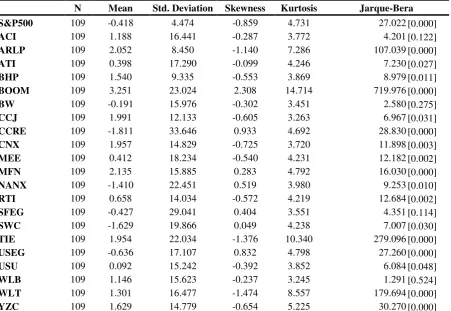
S&P 500 index and the return of the firms‟ descriptive statistics are given in Table 2.
According to the results in Table 2, the lowest monthly return in the period and the highest
deviation belong to CCRE coal firm. According to the kurtosis value, the characteristic of the
whole coal firms returns‟ distribution is observed as fat tail. Jarque-Bera normality test
statistics indicate that coal firms‟ returns do not have a normal distribution except ACI, BW,
[image:12.595.74.526.284.595.2]SFEG and WLB.
Table 2
Descriptive Statistics on Security Returns
N Mean Std. Deviation Skewness Kurtosis Jarque-Bera
S&P500 109 -0.418 4.474 -0.859 4.731 27.022 [0.000]
ACI 109 1.188 16.441 -0.287 3.772 4.201 [0.122]
ARLP 109 2.052 8.450 -1.140 7.286 107.039 [0.000]
ATI 109 0.398 17.290 -0.099 4.246 7.230 [0.027]
BHP 109 1.540 9.335 -0.553 3.869 8.979 [0.011]
BOOM 109 3.251 23.024 2.308 14.714 719.976 [0.000]
BW 109 -0.191 15.976 -0.302 3.451 2.580 [0.275]
CCJ 109 1.991 12.133 -0.605 3.263 6.967 [0.031]
CCRE 109 -1.811 33.646 0.933 4.692 28.830 [0.000]
CNX 109 1.957 14.829 -0.725 3.720 11.898 [0.003]
MEE 109 0.412 18.234 -0.540 4.231 12.182 [0.002]
MFN 109 2.135 15.885 0.283 4.792 16.030 [0.000]
NANX 109 -1.410 22.451 0.519 3.980 9.253 [0.010]
RTI 109 0.658 14.034 -0.572 4.219 12.684 [0.002]
SFEG 109 -0.427 29.041 0.404 3.551 4.351 [0.114]
SWC 109 -1.629 19.866 0.049 4.238 7.007 [0.030]
TIE 109 1.954 22.034 -1.376 10.340 279.096 [0.000]
USEG 109 -0.636 17.107 0.832 4.798 27.260 [0.000]
USU 109 0.092 15.242 -0.392 3.852 6.084 [0.048]
WLB 109 1.146 15.623 -0.237 3.245 1.291 [0.524]
WLT 109 1.301 16.477 -1.474 8.557 179.694 [0.000]
YZC 109 1.629 14.779 -0.654 5.225 30.270 [0.000]
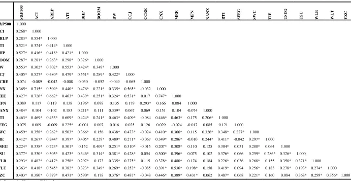
The correlation of the security returns and S&P 500 index are given in Table 3.
According to the results given in Table 3, the companies‟ returns except CCRE, MFN and
SFEG, and the market returns (S&P 500) move parallel and also they are significantly
correlated. Moreover, the returns of CCRE, MFN and SFEG companies move independently
12 Table 3
Correlation among the Returns of the Coal Firms
S &P 5 0 0 A C I A R L P A T I B HP B OO M B W C C J C C R E
CNX M
E E M FN
NANX RT
I S FE G S WC T IE U S E G U S U WL B WL T Y Z C
S&P500 1.000
ACI 0.268* 1.000
ARLP 0.283* 0.554* 1.000
ATI 0.521* 0.324* 0.414* 1.000
BHP 0.527* 0.416* 0.418* 0.421* 1.000
BOOM 0.287* 0.281* 0.263* 0.298* 0.326* 1.000
BW 0.553* 0.302* 0.302* 0.553* 0.424* 0.349* 1.000
CCJ 0.405* 0.527* 0.480* 0.479* 0.551* 0.289* 0.422* 1.000
CCRE 0.074 -0.089 -0.042 -0.008 0.030 -0.052 -0.049 -0.065 1.000
CNX 0.365* 0.715* 0.509* 0.440* 0.476* 0.221* 0.335* 0.565* -0.032 1.000
MEE 0.427* 0.726* 0.662* 0.463* 0.439* 0.251* 0.324* 0.531* 0.017 0.747* 1.000
MFN 0.089 0.117 0.119 0.138 0.196* 0.098 0.135 0.179 0.293* 0.166 0.084 1.000
NANX 0.484* 0.104 0.102 0.183 0.211* 0.111 0.339* 0.067 0.069 0.151 0.104 -0.074 1.000
RTI 0.463* 0.469* 0.433* 0.609* 0.424* 0.241* 0.463* 0.409* -0.084 0.446* 0.463* 0.175 0.206* 1.000
SFEG 0.075 0.009 -0.009 0.225* -0.001 0.007 0.016 0.025 0.126 0.029 -0.024 -0.017 0.085 0.121 1.000
SWC 0.459* 0.358* 0.262* 0.503* 0.366* 0.156 0.438* 0.473* -0.024 0.410* 0.366* 0.115 0.326* 0.348* 0.227* 1.000
TIE 0.412* 0.267* 0.244* 0.397* 0.405* 0.229* 0.489* 0.271* -0.067 0.349* 0.286* -0.010 0.244* 0.411* -0.042 0.297* 1.000
USEG 0.224* 0.338* 0.223* 0.301* 0.152 0.409* 0.251* 0.310* -0.015 0.207* 0.308* 0.110 0.125 0.304* 0.031 0.288* 0.064 1.000
USU 0.377* 0.330* 0.305* 0.423* 0.346* 0.314* 0.381* 0.428* 0.054 0.300* 0.396* 0.075 0.102 0.376* 0.066 0.259* 0.286* 0.326* 1.000
WLB 0.293* 0.482* 0.417* 0.258* 0.297* 0.173 0.335* 0.375* 0.115 0.378* 0.480* 0.174 0.184 0.226* 0.036 0.268* 0.155 0.358* 0.371* 1.000
WLT 0.363* 0.418* 0.545* 0.382* 0.323* 0.349* 0.269* 0.352* -0.085 0.391* 0.536* 0.198* 0.158 0.419* 0.094 0.256* 0.183 0.278* 0.193* 0.274* 1.000
13
Using the Coal Firms‟ return series and the risk-free interest rate, the excess return
series are formed and it is aimed to investigate whether they are stationary or not by using
PP test which is proposed by Phillips and Perron (1988) and KPSS unit root test which is
proposed by Kviatkowski et. al (1992). According to the unit root test results which are
given in Table 4, all the variables that are used in models are observed as stationary.
Table 4
Unit Root Test Results
Variable PP KPSS Variable PP KPSS
RM -8.737* 0.215* MFN -10.216* 0.392*
ACI -8.441* 0.237* NANX -11.538* 0.280*
ARLP -10.528* 0.383* RTI -10.235* 0.323*
ATI -9.488* 0.205* SFEG -6.986* 0.158*
BHP -10.091* 0.162* SWC -9.640* 0.075*
BOOM -11.715* 0.139* TIE -9.584* 0.177*
BW -10.023* 0.122* USEG -10.778* 0.143*
CCJ -8.977* 0.381* USU -9.400* 0.155*
CCRE -13.701* 0.136* WLB -9.457* 0.369*
CNX -9.723* 0.156* WLT -8.536* 0.083*
MEE -8.989* 0.117* YZC -8.915* 0.108*
Unit root tests are examined with constant term model. * indicates that null hypothesis of unit root is rejected at 1% significance level.
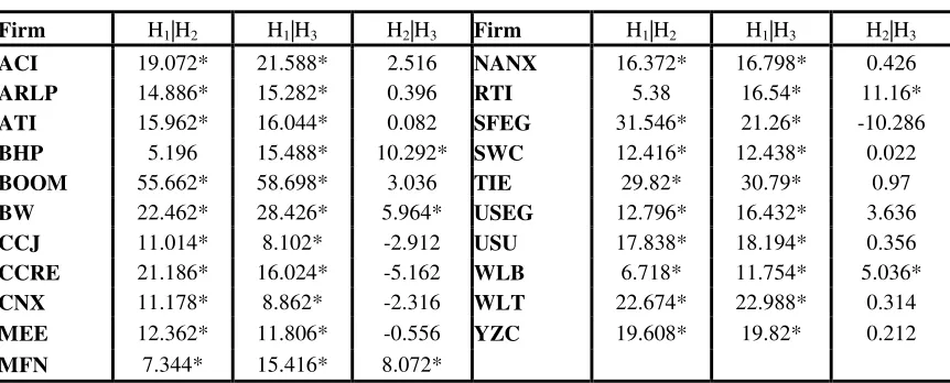
In this study, as there are three different models that are taken into consideration,
the most suitable model should be investigated. For this reason, three models are formed
for all the firms and LR test is used to select the best model. The results of the LR test are
given in Table 5. The Hi|Hj notation in Table 5, shows that in LR test Model i is tested
against Model j. As a result, if test statistics are greater than critical values than null
hypothesis is rejected and superior model is selected as Model j. According to these
results, Model I, linear model shows a low performance and null hypothesis is being
rejected. This result proves that the beta as a measure of systematic risk shows a
14
whether it shows a meaningful difference in both regimes. Consequently, Model II and
Model III provided better results. Not only beta that is calculated for BHP, BW, MFN,
RTI and WLB but also alpha showed variability during low and high volatility periods.
For this reason, Model III is found as the best suitable model for these companies;
[image:15.612.91.522.251.425.2]however, for the rest of the companies Model II gives better results.
Table 5
Likelihood Ratio Test Results
Firm H1|H2 H1|H3 H2|H3 Firm H1|H2 H1|H3 H2|H3
ACI 19.072* 21.588* 2.516 NANX 16.372* 16.798* 0.426
ARLP 14.886* 15.282* 0.396 RTI 5.38 16.54* 11.16*
ATI 15.962* 16.044* 0.082 SFEG 31.546* 21.26* -10.286
BHP 5.196 15.488* 10.292* SWC 12.416* 12.438* 0.022
BOOM 55.662* 58.698* 3.036 TIE 29.82* 30.79* 0.97
BW 22.462* 28.426* 5.964* USEG 12.796* 16.432* 3.636
CCJ 11.014* 8.102* -2.912 USU 17.838* 18.194* 0.356
CCRE 21.186* 16.024* -5.162 WLB 6.718* 11.754* 5.036*
CNX 11.178* 8.862* -2.316 WLT 22.674* 22.988* 0.314
MEE 12.362* 11.806* -0.556 YZC 19.608* 19.82* 0.212
MFN 7.344* 15.416* 8.072*
H1 represents Model I, H2 represents Model II and H3 represents Model III. * indicates that null hypothesis is rejected at 5% significance level.
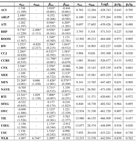
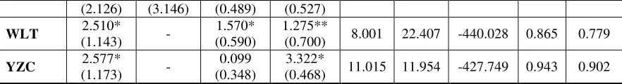
The results of MS-CAPM model are given in Table 6. According to the results in
Table 6, beta parameter, the systematic risk measure shows different results in low and
high volatile periods. Low and high volatile periods are decided according to the standard
error of regression. When the standard error is low, the period is named as low volatility,
and when the standard error is high, the period is named as high volatility.1
1 The normality test, heteroscedasticity and autocorrelation tests are done with the error terms taken from
15
Firstly, if we are to interpret the results of low volatile period; the beta parameter
of the securities of ACI, BOOM, CNX, NANX, RTI, SWC, USEG, USU, and WLB is
greater than one and statistically significant at 5% level. This result indicates that the
firms during the low volatility periods are riskier. This provides a chance to the investors
of such securities to have higher returns. The beta parameter of ATI and BHP firms
which is less than one and statistically significant shows that the securities of such firms
are less risky. Whereas, during the low volatile period, the beta parameters of the
securities of CCJ, CCRE, MFN are less than zero and statistically significant indicating
that the returns of the securities move in the opposite direction to the market return.
During the low volatile period, the beta parameter of ARLP, MEE, SFEG and YZC firms
is not found statistically significant. This result indicates that during the low volatile
period it has no relation with the market return. The betas of CCJ, CCRE and MFN firms
are negative and statistically significant showing that during the low volatile period, the
return of the securities move in the opposite direction to the market.
According to the results during the high volatile period; the beta parameter of the
securities of ATI, BHP, BW, CCJ, CCRE, MEE, RTI, WLT and YZC is found greater
than one. This result shows that during the high volatile periods the systematic risk is
higher. The beta parameter of ARLP and MFN firms is less than one and statistically
significant indicating that during the high volatile period, the systematic risk is lower.
Finally, the beta parameters of ACI, CNX, NANX, SFEG, SWC, TIE, USEG, USU and
WLB are not found statistically significant showing that such firms‟ returns during high
volatile period move independently from the market return. There is a considerable
16
coal firms‟ returns and the market returns with the linear CAPM, then β was going to be
estimated from the MS-CAPM model. This result can be misleading and the risk can be higher
than (or lower) the market making a firm to have lower (or higher) risk than the market. For this
reason, when the CAPM and firms‟ risk level is investigated the existence of the non-linear
[image:17.612.87.529.239.701.2]relation should be taken into consideration.
Table 6
MS-CAPM Results
αlow αhigh βlow βhigh σlow σhigh LogL p1/q1 p2/q2
ACI 1.748
(1.189) -
3.010* (0.601)
-0.444
(0.861) 8.762 12.284 -428.743 0.443 0.705
ARLP 2.490*
(0.692) -
0.352 (0.268)
0.902*
(0.585) 6.100 13.244 -375.264 0.950 0.795
ATI 1.202
(1.197) -
0.946* (0.335)
4.205*
(1.201) 8.697 17.603 -439.426 0.668 0.488
BHP 9.776*
(1.220) -2.496* (1.111) 0.938* (0.161) 1.440*
(0.163) 3.793 5.318 -371.515 0.227 0.548
BOOM 1.071
(1.367) -
1.248* (0.305)
1.131
(2.781) 12.502 49.212 -464.468 0.973 0.805
BW 3.253*
(1.005) -0.820 (2.217) 2.206* (0.215) 1.843*
(0.512) 5.310 16.903 -422.227 0.020 0.216
CCJ 2.284*
(0.820) -
-0.532** (0.292)
1.583*
(0.311) 5.904 9.026 -393.300 0.818 0.928
CCRE -4.260*
(0.535) -
-11.798* (0.087)
1.416*
(0.679) 1.001 30.641 -526.477 0.133 0.952
CNX 2.546*
(1.213) -
2.556* (0.389)
-0.066
(0.580) 9.288 15.143 -435.339 0.878 0.863
MEE 1.109
(1.592) -
-1.059 (0.722)
3.115*
(0.561) 9.610 15.581 -453.225 0.328 0.642
MFN 21.269*
(4.081) 0.686 (1.438) -5.426* (1.001) 0.579**
(0.309) 9.341 13.765 -447.485 0.651 0.969
NANX -0.705
(1.558) -
3.731* (0.515)
1.339
(0.871) 12.310 26.501 -471.450 0.905 0.834
RTI 13.541*
(0.527) 1.029 (1.139) 7.008* (0.097) 1.187*
(0.251) 0.932 11.371 -420.681 0.375 0.972
SFEG -0.522
(0.845) -
0.177 (0.174)
0.210
(1.023) 6.840 18.730 -402.542 0.964 0.895
SWC -0.690
(1.486) -
2.125* (0.387)
1.221
(2.329) 12.934 31.330 -461.720 0.807 0.107
TIE 4.043*
(1.526) -
1.627* (0.361)
3.763
(2.377) 13.980 46.155 -466.509 0.942 0.457
USEG -1.156
(1.384) -
1.174* (0.344)
-2.912
(2.870) 13.077 28.374 -448.899 0.918 0.020
USU 1.156
(1.047) -
1.516* (0.242)
0.990
(0.812) 7.955 20.418 -433.221 0.864 0.758
17
(2.126) (3.146) (0.489) (0.527)
WLT 2.510*
(1.143) -
1.570* (0.590)
1.275**
(0.700) 8.001 22.407 -440.028 0.865 0.779
YZC 2.577*
(1.173) -
0.099 (0.348)
3.322*
(0.468) 11.015 11.954 -427.749 0.943 0.902
* indicates significance level at 5%. The values in parenthesis show the standard errors. σlow shows the standard error of regression
during the low volatile period, σhigh shows the standard error of regression during high volatile period. p1/q1 shows the probability of low volatile period after low volatile period, p2/q2 shows the probability of high volatility period after high volatility period. LogL represents the log likelihood function.
The relation between the returns of the coal firms that are derived from
[image:18.612.86.527.72.132.2]MS-CAPM and market return is also summarized in Table 7.
Table 7
The Relation between Coal Firms and the Market during Low and High Volatility
Firms
Low Volatility High Volatility
Risky Low Risk No Relation with the Market Opposite to the Market
Risky Low Risk No Relation with the Market Opposite to the Market
ACI ● ●
ARLP ● ●
ATI ● ●
BHP ● ●
BOOM ● ●
BW ● ●
CCJ ● ●
CCRE ● ●
CNX ● ●
MEE ● ●
MFN ● ●
NANX ● ●
RTI ● ●
SFEG ● ●
SWC ● ●
TIE ● ●
USEG ● ●
USU ● ●
WLB ● ●
WLT ● ●
YZC ● ●
Results obtained from MS-CAPM are important three aspects. First of all, we
conclude that betas of coal companies are not stable through time and changes related to
volatility of stock return. This result indicates that linear CAPM doesn‟t describe excess
18
should consider time-varying beta to optimize their portfolios because beta obtained from
linear CAPM is found between betas obtained from MS-CAPM. Finally, investors and
academicians should use nonlinear models to forecast stock return of coal companies
because likelihood ratio test results indicate that nonlinear models capture better
behaviors of stock return of coal companies than linear models.
However, these results bring with questions that why the betas of coal companies
are time-varying and why the coal companies behave differently from each others.
Therefore some studies in the literature try to answer these questions. The first
interpretation of these questions suggested by Stattman (1980), Rosenberg et al. (1985),
and Fama and French (1992) emphasizes the book-to-market anomalies in which average
returns on stocks with high ratios of book value to market value are higher than those
with low ratios of book value to market value. It is expected related to finance theory
because companies grow and invest new projects through time and these lead to change
risk profile of companies. Therefore, book-to-market values of companies cause to
change their betas over 10 or 20 years horizon even in short periods.
The second interpretation proposed by Banz (1981) emphasizes the size effect that
the average returns on stocks of small firms are higher than the average returns on stocks
of large firms. The third interpretation argued by Jegadeesh and Titman (1999) is the
momentum effect that stocks with higher returns in previous 12 months (winning stocks)
tend to have higher future returns than stocks with lower returns in the previous 12
months (losing stocks). In this context, Tai (2003), Ang and Chen (2007), In and Kim
(2007) and Abdymomunov and Morley (2009) determine book-to-market, the size effect
19
Liu (2004) argued that discounting cash-flows of firms lead to change market risk
premiums, risk-free rates and betas over time.
Also, it is well known that changes in the oil price have significant effect on stock
returns of energy companies and any shocks in the oil price lead to change betas of
energy companies over time. Faff and Brailsford (1999), Sadorsky (2001), Trück (2008)
and Boyer and Fillon (2007) determine that changes in the oil price effect positively and
significantly to stock returns of energy companies.
5. Conclusion
CAPM which measures the relationship between securities‟ return and the market
return has a significant place in finance theory. In CAPM, the systematic risk of the
securities is measured with beta parameter and with the value of the parameter; the risk
level of the securities can be interpreted accordingly. In traditional finance theory, the
return of the securities and the market return relation are assumed as linear and when the
return of the securities increase than systematic risk also increases. In recent years, with
the development of the behavioral finance theory, the return and risk relation is proved
not to be linear at all times and with the effect of the anomalies in the market, this
relation is found in opposite direction. On the other hand, with the development in
nonlinear time series analysis, in lots of studies, beta shows variability in high and low
volatile periods. Especially when the return of the securities and the risk are taken as
linear, the beta parameter can be misleading. For this reason, this study investigates the
risk level of the securities of coal firms that are traded in U.S. securities markets with the
linear and nonlinear models. According to the results, the relation between the return of
20
models are used. The first one is the CAPM where alpha is constant and beta is a
variable. In the second non-linear model, alpha and beta parameters are assumed to be
variable in high and low volatile periods. According to the findings, the first model gave
better results and only BHP, BW, MFN, RTI and WLB fit better to the second model.
To summarize the results from the MS-CAPM, it can be noted that in low and
high volatile periods BW, RTI and WLT firms have higher systematic risk. ACI, BOOM,
CNX, NANX, SWC, TIE, USEG, USU and WLB firms in the periods of low volatile
period have higher systematic risk whereas, ATI, BHP, CCJ, CCRE, MEE and YZE
firms have low systematic risk during low volatile periods. ARLP firm in both periods,
MEE, SFEG and YZC firms, and the return of the MFN firms during high volatile period
is observed as unrelated. Finally, the return of the securities of CCJ, CCRE and MFN
and the market return move completely in the opposite direction during low volatility
period.
REFERENCES
Abdymomunov, A. and Morley, J. C. (2009). “Time-variation of CAPM betas across market volatility regime for book-to-market and momentum portfolios”, http://artsci.wustl.edu/~morley/am.pdf, (Access Date: May 01, 2010).
Alexander, G. J., Benson, P. G. and Eger, C. E. (1982). “Timing decisions and the behavior of mutual fund systematic risk”, Journal of Financial and Quantitative Analysis, 17: 579-602.
Ang, A. and Chen, J. (2007). “CAPM over the long run: 1926-2001”, Journal of Empirical Finance, 14: 1-40.
Ang, A. and Liu, J. (2004). “How to discount cashflows with time-varying expected
returns”, Journal of Finance, 59: 2745-2783.
Balat, M. and Ayar, G. (2004). “Turkey‟s coal reserves, potential trends and pollution
problems of Turkey”, Energy Exploration & Exploitation, 22: 71-81.
Banz, R.W. (1981). “The relation between return and market value of common stocks”,
Journal of Financial Economics, 9: 3-18.
21
Boyer, M. and Filion, D. (2007). “Common and fundamental factors in stock returns of Canadian oil and gas companies”, Energy Economics, 29: 428-453.
Chen, S. N. (1982). “An examination of risk-return relationship in bull and bear markets using time-varying security betas”, Journal of Financial and Quantitative Analysis, 17: 265-286.
Chen, S.-W. and Huang, N.-C. (2007). “Estimates of the ICAPM with regime-switching betas: evidence form four pacific rim economies”, Applied Financial Economics, 17: 313-327.
Fabozzi, F. J. and Francis, J. C. (1977). “Stability tests for alphas and betas over bull and bear market conditions”, Journal of Finance, 32: 1093-1099.
Faff, R. and Brailsford, T. (1999). “Oil price risk and the Australian stock market”, Journal of Energy Finance and Development, 4: 69-87.
Fama, E. F. and French, K.R. (1992). “The cross-section of expected stock returns”, Journal of Finance, 47: 427-465.
Fearnley, T. A. (2002). “Tests of an international capital asset pricing model with stocks and government bonds and regime switching prices of risk and intercepts”, Graduate Institute of International Studies and International Center for Financial Asset Management and Engineering (FAME), Research Paper, No. 97, Available at: http://papers.ssrn.com/sol3/papers.cfm?abstract_id=477485.
Fridman, M. (1994). “A two state capital asset pricing model”, IMA Preprint Series, No. 1221.
Galagedera, D. U.A. and Fuff, R. (2005). “Modeling the risk and return relation conditional on market volatility and market conditions”, International Journal of Theoretical and Applied Finance, 8: 75–95.
Galagedera, D. U.A. and Shami, R. (2003). “Association between Markov regime-switching market volatility and beta risk: evidence from Dow Jones industrial securities”, Monash Econometrics and Business Statistics Working Paper No. 20/03, Monash University, Department of Econometrics and Business Statistics.
Gu, L. (2005). “Asymmetric Risk Loadings in the Cross Section of Stock Returns”, Colombia University Job Market Paper, Available at: http://papers.ssrn.com/sol3/papers .cfm?abstract_id=676845
Hamilton, J. D. (1994). Time Series Analysis. Princeton University Press, New Jersey. Hess, M. K. (2003). “What drives Markov regime-switching behavior of stock markets? The Swiss case”, International Review of Financial Analysis, 12: 527-543.
http://finance.yahoo.com (Access Date: January 5, 2009).
http://mba.tuck.dartmouth.edu/pages/faculty/ken.french/ (Access Date: January 5, 2009).
22
Huang, H.-C. (2001). “Tests of CAPM with nonstationary Beta”, International Journal of Finance and Economics, 6: 255-268.
Huang, H.-C. (2003). “Tests of regime-switching CAPM under price limits”, International Review of Economics and Finance, 12: 305-326.
Huang, H.-C. and Cheng, W.-H. (2005). “Tests of the CAPM under structural changes”, International Economic Journal, 19: 523-541.
Hwang, S., Satchell, S. E. and Pereira, P. L. V. (2007). “How persistent is stock return volatility? An answer with Markov regime switching stochastic volatility models”, Journal of Business Finance & Accounting, 34: 1002–1024.
In, F. and Kim, S. (2007). “A note on the relationship between Fama-French risk factors
and innovations of ICAPM state variables”, Finance Research Letters, 4: 165-171.
Ishijima, H., Takano, E. and Taniyama, T. (2004). “The growth of optimal asset pricing model under regime switching: with an application to J-REITs”, Daiwa International Workshop on Financial Engineering No.15710120.
Jagannathan, R. and Wang, Z. (1996). “The conditional CAPM and the cross-section of expected returns”, Journal of Finance, 51: 3–54.
Jegadeesh, N. and Titman, S. (1999). “Profitability of momentum strategies: An evaluation of alternative explanations”, Working Paper, University of Texas at Austin. Krolzig, H.-M. (1997). Markov-Switching Vector Autoregressions Modelling, Statistical Inference, and Application to Business Cycle Analysis. Springer, Berlin.
Kwiatkowski, D., Phillips, P.C.B., Schmidt, P. and Shin, Y. (1992). “Testing for the null hypothesis of stationarity against the alternative of a unit root”, Journal of Econometrics,
54: 159–178.
Levy, R. A. (1971). “On the short-term stationarity of beta coefficients”, Financial Analysts Journal, 27: 55-62.
Li, M.-Y. L. (2007). “Volatility states and international diversification of international stock markets”, Applied Economics, 39: 1867–1876.
Lintner, J. (1965a). “The valuation of risk assets and the selection of risky investments in stock portfolios and capital budgets”,Review of Economics and Statistics, 47: 13–47. Lintner, J. (1965b). “Security prices, risk and maximal gains from diversification”,
Journal of Finance, 20: 587–616.
Liow, K. H. and Zhu, H. (2007). “Regime switching and asset allocation”, Journal of Property Investment & Finance, 25: 274-288.
Phillips, P.C.B. and Perron, P. (1988). “Testing for a unit root in time series regression”, Biometrika, 75: 335–346.
Rosenberg, B., Reid, K. and Lanstein, R. (1985). “Persuasive evidence of market
23
Sadorsky, P. (2001). “Risk factors in stock returns of Canadian oil and gas companies”, Energy Economics, 23: 17–28.
Shami, R. and Galagedera, D. U. A. (2004). “Beta risk and regime shift in market volatility”, Economic Society Australasian Meetings 126, Available at: http://papers.ssrn .com/sol3/papers.cfm?abstract_id=612022
Sharpe, W. F. (1964). “Capital asset prices: A theory of market equilibrium under conditions of risk”, Journal of Finance, 19: 425–442.
Stattman, D. (1980). “Book values and stock returns”, The Chicago MBA: a Journal of Selected Papers, 4: 5-45.
Tai, C. S. (2003). “Are Fama-French and momentum factors really priced?”, Journal of Multinational Financial Management, 13: 359-384.
Tiwari, A. (2006). “Investing in mutual funds with regime switching”. Available at: http://www.biz.uiowa.edu/faculty/atiwari/InvestinginMFunds.pdf.
Trück, S. (2008). “Oil price dynamics and returns of renewable energy companies”,
http://www.firn.net.au/resources/pdfs-papers-slides/Trueck_RD_2008.pdf, (Access Date: May 01, 2010)
Wilson, C. A. and Featherstone, A. M. (2006). “Adjusting the CAPM for threshold effects: An application to food and agribusiness stocks”, Purdue University Staff Paper No. 06-08.
World Energy Outlook (2008). http://www.worldenergyoutlook.org/docs/weo2008/ WEO2008_es_english.pdf, (Access Date: May 15, 2009)
Yılmaz, A. O. and Uslu, T. (2007). “The role of in energy production-consumption and