The Instability in the Monetary Policy Reaction Function and the Estimation of Monetary Policy Shocks

Munich Personal RePEc Archive

The Instability in the Monetary Policy

Reaction Function and the Estimation of

Monetary Policy Shocks

Kishor, N. Kundan and Newiak, Monique

University of Wisconsin-Milwaukee

18 June 2009

Online at

https://mpra.ub.uni-muenchen.de/17643/

The Instability in the Monetary Policy Reaction

Function and the Estimation of Monetary Policy

Shocks

y

N. Kundan Kishor

University of Wisconsin-Milwaukee

Monique Newiak

University of Munich

Abstract

This paper uses the conventional wisdom about the shift in the monetary policy stance in 1979 to compute monetary policy shocks by estimating di¤erent monetary policy reaction functions for the pre-1979 and post-1979 time periods. We use the information from the internal forecasts of the Federal Reserve to derive monetary policy shocks. The results in this paper show that a monetary policy shock in the pre-1979 period a¤ects output and prices much more strongly and quickly than what has been reported in the literature for the full sample. Our …ndings suggest that the dynamic response of output and prices to a monetary policy shock declined signi…cantly between 1980-2001. We argue that this diminished response to the monetary policy shock is the result of a successful monetary policy that has led to a less volatile economy.

Kishor: Department of Economics, Bolton Hall, Box 0413, University of Wisconsin-Milwaukee, Milwau-kee, WI-53201 (Email: kishor@uwm.edu). Newiak: Ludwig Maximilian University Munich, Department of Economics, Munich Graduate School of Economics, Kaulbachstraße 45, 80539 Munich, Germany (Email: info@monique-newiak.de)

1

Introduction

Monetary policy is not exogenously given, but largely driven by policy makers’ reactions

to macroeconomic conditions (Bernanke, Gertler and Watson (1997)). In order to measure

the impact of monetary policy, we therefore need to estimate its component that does not

respond endogenously to the changes in the macroeconomic environment. To overcome the

problem of endogeneity, di¤erent approaches have been proposed. One notable approach is

the identi…cation of monetary policy shocks due to Romer and Romer (2004)1_{. Romer and}

Romer (2004; RR hereafter) derive their measure of monetary policy shocks by regressing

changes in the intended federal funds rate on information about output growth, in‡ation and

the unemployment rate for every regular Federal Open Market Committee (FOMC) meeting

in the period between 1969 and 1996.2 _{The residuals from this regression show the change in}

the intended federal funds rate not taken in response to information about future economic

developments. They therefore constitute a measure of monetary policy shocks.

The results of RR’s analysis are appealing from a theoretical point of view: the "price

puzzle"3 _{disappears, and output also responds appropriately to monetary policy shocks.}

However, RR’s work is based on two simplifying assumptions: …rst, they assume that the

monetary policy makers’ response to movements in in‡ation and output has not changed for

the whole sample, and secondly, that the response of prices and output to monetary policy

shocks remained the same for the whole sample. This contradicts recent literature which

…nds evidence of a change in the monetary policy reaction function within the examined

period4 _{and a change in the response of output and prices to monetary policy shocks}5_.

1_{Other popular approaches include the recursive VAR approach of Christiano, Eichenbaum, and Evans}

(1996), the structural VAR approach of Bernanke and Mihov (1998) and Boivin and Giannoni (2006), and the Federal Funds Futures market approach of Kuttner (2001).

2_{The information about output growth, in‡ation and the unemployment rate is represented by the}

Green-book forecasts that are prepared by the Federal Reserve sta¤, and presented to the policymakers before each FOMC meeting.

3_{Price puzzle refers to the positive response of prices to a monetary policy shock.} 4_{Clarida, Gali and Gertler (2000), Orphanides (2001, 2002, 2004).}

5_{See the NBER working paper version (no. 5145, June 1995) of Bernanke and Mihov (1998), Barth and}

Our approach in this paper is based on the compelling evidence that the monetary policy

response to changes in macroeconomic conditions has changed since Paul Volcker took over

the chairmanship of the Federal Reserve in 1979 and that the Federal Reserve has played

a signi…cant role in the stabilization of the macroeconomy between 1980-2001. We also

recognize that the macroeconomic stability experienced in the U.S. between 1980-2001 might

have changed the response of output and prices to monetary policy shocks. Our approach of

sub-sample analysis allows us to examine the dynamic response of macroeconomic variables

to monetary policy shocks across the two sub-samples.

Using RR’s approach, we derive monetary policy shocks by estimating di¤erent monetary

policy reaction functions for the pre-1979 and post-1979 periods. Our …ndings suggest that

ignoring the instability in the monetary policy reaction function can provide a misleading

e¤ect of the monetary policy shock on output and prices for the whole sample. We …nd that

the estimate of monetary policy shocks for the whole sample is disproportionately a¤ected

by the pre-1979 period shocks, and hence the response of output and prices to a monetary

policy shock for the whole sample in RR’s analysis mainly re‡ects the impact of the shocks

estimated from the …rst sub-sample. If monetary policy shocks are estimated using di¤erent

sub-samples, we …nd that the response of prices to a monetary policy shock is signi…cant and

in the right direction in both sub-samples. However, the e¤ect on prices is much weaker in the

second sub-sample. The response of output to monetary policy shocks is stronger and quicker

in the …rst sub-sample than what has been reported by RR for the whole sample period.

In the second sub-sample, however, the e¤ect of a monetary shock on output disappears

completely.

Consequently, our results indicate that the dynamic response of output and prices to

monetary policy shocks computed from the internal forecasts of the Federal Reserve has

declined substantially since 1980. This result is consistent with what other researchers

including Bernanke and Mihov (1998), and Boivin and Giannoni (2002, 2006) have found

using di¤erent methodologies for the estimation of monetary policy shocks.

We argue that the smaller impact of monetary policy shocks on output and prices do

not in any way re‡ect the reduction in the potency of monetary policy. In fact, the decline

in the responsiveness may itself be the result of a very successful monetary policy. If the

systematic component of monetary policy is perfectly successful, then the goal variables

in-cluding output and prices would become a constant. In that case we would therefore observe

a zero correlation between monetary policy shocks and output and prices. To illustrate this

point, we present a very simple New Keynesian model where we show that the reduction

in the response of output and prices to monetary policy shocks may arise from stabilizing

monetary policy6_.

The rest of this paper is organized as follows: section 2 gives an overview of the approach

by Romer and Romer (2004) to estimate monetary policy shocks; section 3 presents the

estimation and analysis of monetary policy shocks for di¤erent sub-periods; section 4 presents

a simple model to motivate the main results of the paper, and section 5 concludes.

2

Estimation of Monetary Policy Shocks

We follow RR’s approach for the estimation of monetary policy shocks. RR derived the

change in the intended federal funds rate for every regular FOMC meeting by using narrative

evidence from the FOMC meetings, the FOMC transcripts and the Greenbook. The changes

in the intended federal funds rate from meeting to meeting are regressed on the Greenbook

forecasts of in‡ation, output growth and the unemployment rate:

Mf f_m = + f f b_m+

2

X

i= 1

i Myemi+

2

X

i= 1

i(My_emi M_ey_{m 1};i)

+

2

X

i= 1

'iemi+

2

X

i= 1

i(emi em 1;i) + eum0+"m: (1)

6_{Using a structural VAR model, Bovin and Giannoni (2006) show that the diminished response of output}

In (1) M f f_m represents the change in the intended federal funds rate, f f b_m is the level of

the intended federal funds rate before the meeting,Mye_miande_miare the forecasts of output

growth and in‡ation, which are included for the previous and current quarter as well as for

two quarters ahead. Mye_mi Mey_{m 1;i} ande_mi e_{m 1;i}are the revisions in the forecasts for a

certain quarter from the last to the current meeting, and um0 is the current quarter estimate

of the unemployment rate. The residuals "m represent the monetary policy shocks arising

from every meeting.

The e¤ect of a monetary policy shock on prices and output is analyzed by estimating a

VAR that has three variables; the log of industrial production, the log of the PPI for …nished

goods and the measure of the monetary policy shock derived from the above method7_{. Since}

the federal funds rate enters the VAR in levels the shocks are converted into monthly shocks

and cumulated. In what follows, we use the above approach by RR to analyze the results

with an extended data set (1969-2001).

As a …rst step, we make sure that the extension of the data set does not alter the main

results obtained by RR. When we compare the shocks computed with our sample to the

ones by RR for 1969-1996, we …nd a correlation of 0.990 for the cumulated shocks. They

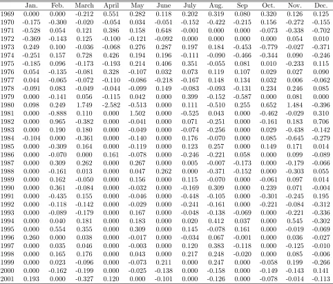
are plotted in …gure 1. The monthly shock series can be found in table 1. Figure 3 presents

the impulse-response functions for the estimated VAR system. They show the impact of the

cumulated shock on output and the price level for the period between 1969 and 2001. Not

surprisingly, the results for the larger data set are qualitatively similar to what RR report in

their paper. After a slight increase during the …rst seven months, output shows a negative

response with a t-statistic of over 2 after the …rst year. The peak response of output is 2.1

percent in month 23. It returns to its initial level after about three years. Prices respond

only slightly, irregularly, and mostly insigni…cantly in the …rst seven months. Afterwards, we

observe a negative response throughout which becomes signi…cant after month 27 and …nd

an e¤ect of -4.4 percent after 48 months. Thus, considering the sample period 1969-2001 as

a whole, the responses of output and prices to monetary shocks are compatible with what

monetary theory would predict.

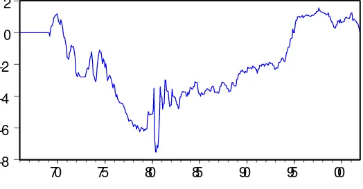
But what drives this almost text-book like result for the whole period? The cumulated

monetary policy shocks plotted in …gure 1 give an answer to this question. They reveal

the problem associated with RR’s estimation of monetary policy shocks by using a single

monetary policy reaction function spanning the whole time period. Shocks are either

persis-tently negative or positive with an obvious turning point around 1979, which is consistent

with the compelling anecdotal evidence on the changes in the monetary policy around that

time. Keeping in mind that the monetary policy shocks are the residuals from a monetary

policy reaction function, the interpretation of this graph is straight forward. Since monetary

policy shock is the di¤erence between the intended federal funds rate and the …tted value

of the intended federal funds rate, we get consistently negative values of the residuals for

the pre-1979 period. By construction, the use of whole sample leads to a lower value of the

…tted federal funds rate in the second sub-sample, and hence the residuals are consistently

positive. The use of the full sample to estimate the monetary policy shocks would give the

impression of a more aggressive response to in‡ation and real activity movements than it

originally was during the …rst sample.

Thus the results of the VAR using the original approach by Romer and Romer (2004)

have one main drawback: They do not take into account the change in the macroeconomic

environment that took place around 1979. The next two sections consider this problem.

3

Changes in the Conduct and Impact of Monetary

Policy

Recent literature supports the view that there has been a structural shift in the way

monetary policy has responded to the movements in in‡ation and output since Paul Volcker

took over the chairmanship of the Federal Reserve. Clarida, Gali and Gertler (2000)

esti-mate a forward-looking policy rule for the periods before and during the Volcker-Greenspan

era in order to evaluate monetary policy’s e¤ectiveness. Their results suggest that in the

with Paul Volcker’s regime, monetary policy played a stabilizing role in containing

in‡a-tion. Orphanides (2000, 2001 and 2004) criticizes Clarida, Gali, and Gertler’s results on

the ground that monetary policy makers are constrained by the availability of the real-time

data. He argues that the use of revised data in their paper provides misleading estimates

of the monetary policy reaction function’s coe¢cients. Orphanides’ results indicate that it

was the aggressive response to movements in the output gap that might have created the

in‡ationary environment in the pre-1979 era, as the response to in‡ation was not statistically

di¤erent across di¤erent sub-periods. Though the conclusions of the papers are certainly

dif-ferent, both approaches reveal that the policy-makers’ response to changes in macroeconomic

variables has changed over time.

The evidence presented in the previous section supports the conventional wisdom that

there was a fundamental shift in the way the Fed responded to in‡ation and the output gap

since Paul Volcker became the chairman of the Federal Reserve. In addition, we perform a

Chow test for a structural break in coe¢cients of equation (1) in the third quarter of 1979.

The test rejects the null hypothesis of no structural break in the third quarter of 1979 with

a p-value of 0.000. Therefore we estimate separate reaction functions for the pre-Volcker

and the Volcker-Greenspan periods for the derivation of the monetary policy shocks. Apart

from breaking the sample into two sub-periods and using a larger data set, we use the same

methodology as Romer and Romer (equation 1). Since performing the estimation for two

time periods (1969-1979 and 1979-2001) makes the sub-samples substantially shorter, we use

24 lags instead of 36 lags in the VAR system. We therein adopt a middle ground in the lag

length selection: Christiano, Eichenbaum and Evans (1996) choose 12 lags in their study of

monetary policy shocks, whereas RR choose 36 lags in their estimation.

Following the methodology described in section 2, we initially estimate monetary policy

shocks for both sub-periods. The monthly shock series thus obtained is given in table 2. We

plot the cumulated monthly shock series in …gure 3 and do not …nd an obvious period of

persistently positive or negative shocks. Supported by the graphical evidence we …nd that

whole sample (0.130). The correlation di¤ers remarkably for the pre-1979 (correlation of

0.514) and the post-1979 (correlation of only 0.042) periods.

To analyze the impact of a monetary policy shock on output and prices, a VAR system

is estimated that includes the log of industrial production, the log of the PPI for …nished

goods and the new cumulated monetary shocks derived from two di¤erent monetary policy

reaction functions for pre-1979 and post-1979 sub-periods.

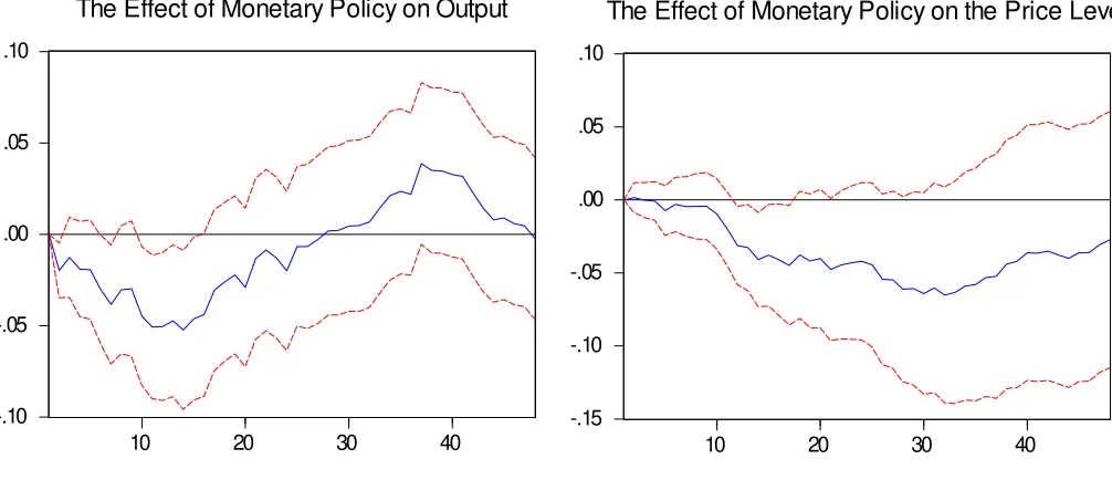
The results suggest that the e¤ect of a monetary policy shock is signi…cantly di¤erent

across the two time periods: For the pre-1979 sub-sample, we …nd an immediate and negative

response of output to a one unit monetary policy shock which becomes signi…cant beginning

in month 6 (…gure 4). The peak e¤ect of a 5.2 percent decline in month 14 is much stronger

and quicker than the response for the whole sample period and for one policy reaction

function. Interestingly, the e¤ect on output dies out at the beginning of the second year and

becomes positive and insigni…cant in month 28. The response of prices is negative beginning

with the second month and becomes signi…cant within a year. The price e¤ect peaks in

month 32 with a response of -6.5 percent and begins to die out afterwards.

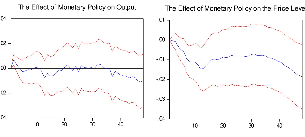
The results for the second period are entirely di¤erent. If we look at the second

sub-sample beginning in July 1979 (…gure 5), we …nd that the response of output to the monetary

contraction is throughout tiny, irregular, and insigni…cant. For in‡ation the negative e¤ect

is small, but becomes signi…cant in month 7 and stays signi…cant until month 14. There is

also a slightly signi…cant e¤ect at the end of the fourth year. Note that the peak e¤ect of

less than 1:5 % in month 12 is much smaller as compared to the pre-1979 sub-sample.89

It has been argued that the period of non-borrowed reserves targeting (1979-1982), also

known as the "Volcker Experiment" was a period of excessive volatility, and it might have

played a big role in the estimation of monetary policy shocks. This problem has been

8_{The …rst part of the e¤ect on prices is consistent with current literature on price changing behavior such}

as by Taylor (1999), Nakamura and Steinsson (2006) and Bils and Klenow (2004).

9_{We also performed a similar analysis by estimating monetary shocks with a single reaction function but}

emphasized by Bernanke and Mihov (1998), who state that the federal funds rate should not

be used as a monetary policy indicator for the time period between 1979 and 1982. Although

the Chow test of a structural break in coe¢cients of equation (1) at the end of 1982 clearly

fails in rejecting the null hypothesis of no structural break (p-value of 0.38), we want to

make sure that the dynamic responses reported above are not driven by the huge variation

in the monetary shocks from this short sample. We therefore perform the above analysis

for the post-1982 sub-period. We …nd that the e¤ect of a monetary policy shock on prices

to be tiny and insigni…cant throughout. The response of output is signi…cantly positive for

the …rst eight months and insigni…cant afterwards.10 _{Thus eliminating the three years of}

non-borrowed reserves targeting makes the change in the response of output and prices to

the unsystematic part of monetary policy even more obvious: Not only does the e¤ect on

prices decrease – it vanishes completely. Not only does the e¤ect on output disappear – the

response partially even reverses its sign.

Consequently, our results indicate that if the monetary policy shocks are estimated using

di¤erent reaction functions for the pre-1979 and the post-1979 time periods, then the response

of output and prices changes signi…cantly across these two sub-periods. Monetary policy

shocks in‡uenced prices almost "textbook-like" throughout the whole period from 1969 to

2001, though the response of the prices was smaller in the second period than in the …rst.

In contrast, monetary policy shocks had a signi…cant e¤ect on output only in the …rst

sub-sample. Overall our results show that the dynamic response of output and prices to monetary

policy shocks has declined signi…cantly in the second sub-period.

4

Has Monetary Policy Lost its E¤ectiveness?

The empirical evidence presented in the previous sections suggests that the response of

output and prices to monetary policy shocks has decreased considerably since 1980. Does this

imply that the Federal Reserve has partly lost its e¤ectiveness in controlling the economy?

10_{We also estimate the dynamic response of output and prices to monetary policy shocks estimated}

Our results certainly do not imply that. In fact, the reduction in the response to monetary

policy shocks may result from the success of systematic monetary policy in dampening

eco-nomic ‡uctuations. To illustrate this point, consider an extreme example. If monetary policy

is perfectly successful, then it would make the goal variable (output or price) a constant11_.

By construction, a constant is uncorrelated with any variable, and thus it will be

uncorre-lated with monetary policy shocks. Therefore if systematic monetary policy was perfectly

successful in stabilizing the economy, we would not …nd any correlation between monetary

policy shocks and in‡ation and output.

To stress this point, we consider a simple New Keynesian model with a dynamic IS-curve

(2) and the New Keynesian Phillips curve (3)12_:

yt = Etyt+1 rt+gt; >0 (2)

t = Et t+1+ yt+ut; (3)

where ytis output, tis the rate of in‡ation, and rtis the real interest rate. All variables are

in terms of percent deviations from their long-run values. Output is negatively correlated

with the real interest rate and also depends on expected future output, as consumers want

to smooth their consumption over time. The parameter is associated with the elasticity of

intertemporal substitution in consumption. In‡ation depends positively on future

expecta-tions about in‡ation (discounted with the time preference factor ) and is positively linked

to the IS-curve through the output gap. The positive parameter summarizes a plethora

of parameters from the New Keynesian model.13 _{The zero-mean disturbance terms g} t and

ut can be interpreted as demand and cost-push shocks, respectively. Iterating equation (1)

forward, we obtain

yt = rLt +gt (4)

where

rL t =Et

" 1

X

j=0 rt+j

#

11_{Kishor and Kochin (2007).} 12_{Clarida, Gali, Gertler (1999).}

represents the long-run real interest rate which is determined by the expected path of the

short-term interest rates. Equation (4) implies that output is determined by the long-run

interest rate. Similarly, we can iterate (2) forward and …nd that in‡ation is determined by

a weighted sum of expected deviations of output from its natural level:

t=Et

" 1

X

k=0

k

yt+s

#

+ut: (5)

In our example, the central bank conducts monetary policy by setting short-term interest

rates. Monetary policy actions can alter the path of expected short-term interest rates, and

hence in‡uence the long-term interest rate. It has been suggested by Taylor (1993) that

monetary policy follows an interest rate rule of the following type:

rt= yyt+ t+"t: (6)

yand represent the magnitudes of the response of the central bank to deviations of output

from its natural level and to in‡ation. "t is the monetary policy shock which is assumed to

be uncorrelated with the demand shockgtand the cost-push shockut. Combining equations

(4), (5) and (6), we obtain

yt =

gt ut "t

1 + _y+ (7)

t =

gt+ (1 + y)ut "t

1 + _y + : (8)

The above expressions imply that equilibrium output and in‡ation depend on demand,

cost-push and monetary policy shocks, as well as on the parameters , , y and . An

unexpected unit increase in the short-term interest rate ("t= 1) reduces equilibrium output

by =(1 + _y+ ), and decreases in‡ation by =(1 + _y+ ). A reduction in the

impact of monetary policy shocks can arise through di¤erent channels: a reduction in or

or a higher value of _y or . If monetary policy has become less potent, then, the lower

output response is due to a smaller elasticity of intertemporal substitution in consumption

to higher values of y or , then it is not related to the degree of potency of monetary

policy. In this case, the lower response of output to monetary policy shocks simply re‡ects

the greater willingness on the part of the monetary policymakers to neutralize ‡uctuations

in output and in‡ation. In the extreme case, the central bank could, for instance, perfectly

stabilize output and in‡ation by letting become very large.

There is a compelling evidence in support of the stabilizing role of monetary policy

in the U.S. since 1980. The monetary policy literature suggests that the Federal Reserve

has responded aggressively to expected movements in output and in‡ation to stabilize the

economy since 198014_{. Therefore the evidence of a decrease in the response of output and}

prices to monetary policy shocks is likely not due to less potency of monetary policy, but a

result of successful monetary policy and its e¤ectiveness in stabilizing in‡ation and output.

This explanation of lower responses of output and in‡ation to monetary policy shocks is

consistent with the results obtained by other researchers in the monetary policy literature15_.

5

Conclusions

In this paper, we revisit the estimation of monetary policy shocks using the methodology of

Romer and Romer (2004) for the sample that runs from 1969 through 2001. We utilize the

conventional wisdom about a fundamental shift in the monetary policy formulation in the

U.S. after the appointment of Paul Volcker as the chairman of the Federal Reserve in 1979 to

divide the sample into pre-Volcker and Volcker-Greenspan sub-periods. Romer and Romer

(2004) assumed similar responses of the Federal Reserve to movements in in‡ation and the

output gap for the whole sample period, 1969-1996, for the estimation of their monetary

policy shocks.

Our results indicate that the monetary policy shocks from the pre-Volcker sub-sample

disproportionately a¤ect the result for the whole sample when a single monetary policy

re-14_{Clarida, Gali, and Gertler (2000), Boivin and Giannoni (2002, 2006), Favero and Rovelli (2003), Senda}

(2005).

15_{For example, Barth and Ramey (2000), Boivin and Giannoni (2002, 2006), Gertler and Lown (2000),}

action function is used to estimate them. If monetary policy shocks are estimated using

di¤erent reaction functions for the two di¤erent sub-samples, the results are strikingly

di¤er-ent. We …nd that prices and output respond almost in a textbook fashion for the pre-Volcker

period. The response of output to a monetary policy shock is faster in the …rst sub-sample

than what has been reported by Romer and Romer for the whole sample period. In contrast

to Romer’s and Romer’s …ndings, our results show that output’s response to a monetary

policy shock in the second period is very small and insigni…cant, whereas the response of

prices is signi…cant and in the right direction. However, the magnitude of the price response

is much smaller as compared to the …rst sub-sample and vanishes completely when the three

years of non-borrowed reserves targeting are excluded from the sample. The decline in the

magnitude of the response of prices and output to monetary policy shocks is consistent with

the results of Boivin and Giannoni (2005), and Bernanke and Mihov (1998).

We stress that the decline in the response of output and in‡ation does not mean that

monetary policy has become less e¤ective after 1979. On the contrary, it can be shown that

the lack of response to theunsystematic part of monetary policy might be due to the success

of the systematic part of monetary policy in stabilizing output and in‡ation.

Thus the results in this paper present an interesting conundrum about the impact of

monetary policy shocks. The exogenous shocks to monetary policy are estimated to

sepa-rate it from the endogenous response of monetary policy to changes in the macroeconomic

environment. The role of the systematic monetary policy or the endogenous movements in

the federal funds rate is to stabilize the economy. If the monetary policy is perfectly

success-ful in its objective, then the important question of what happens after an exogenous shock

to monetary policy becomes hard to answer, as the correlation between a perfectly stable

variable and the monetary policy shock would be zero. On the other hand, if the monetary

policy is not successful, then there remains enough variation on the goal variable to capture

References

[1] Barth, Marvin, and Valerie A. Ramey (2001), "The Cost Channel of Monetary

Trans-mission", NBER Macroeconomics Annual 2001.

[2] Bernanke, Ben S., and Alan S. Blinder (1992), "The Federal Funds Rate and the

Chan-nels of Monetary Transmission" The American Economic Review, Vol. 82, No. 4 (Sep.),

901-21.

[3] Bernanke, Ben S., Mark Gertler, Mark Watson, Christopher A. Sims, and Benjamin M.

Friedman (1997), "Systematic Monetary Policy and the E¤ects of Oil Price Shocks",

Brookings Papers on Economic Activity, Iss. 1, 91-157.

[4] Bernanke, Ben S., and Ilian Mihov (1998), "Measuring Monetary Policy", The Quarterly

Journal of Economics, Vol. 113, No. 3 (Aug.), 869-902.

[5] Bils, Mark and Peter J. Klenow (2004), "Some Evidence on the Importance of Sticky

Prices", Journal of Political Economy, Vol. 112, No. 5, 947-985.

[6] Boivin, Jean, and Marc P. Giannoni (2002), "Assessing Changes in the Monetary

Trans-mission Mechanism: A VAR Approach", Economic Policy Review, May, 97-107.

[7] Boivin, Jean, and Marc P. Giannoni (2006), "Has Monetary Policy Become More

E¤ec-tive?", The Review of Economics and Statistics, Vol. 88, No. 3 (Aug.), 445-62.

[8] Christiano, Lawrence, Martin Eichenbaum and Charles Evans (1996), "Monetary policy

shocks: what have we learned and to what end?", In: Michael Woodford and John

Taylor, eds, Handbook of Macroeconomics North Holland.

[9] Clarida, Richard, Jordi Gali, and Mark Gertler (1999), "The Science of Monetary Policy:

A New Keynesian Perspective", In: Journal of Economic Literature, Vol. 37 (December

[10] Clarida, Richard, Jordi Gali and Mark Gertler (2000), "Monetary Policy Rules and

Macroeconomic Stability: Evidence and Some Theory", Quarterly Journal of

Eco-nomics, Vol. 115, No. 1 (Feb.), 147-80.

[11] Cochrane, John H. (1998), "What do the VARs Mean? Measuring the Output E¤ects

of Monetary Policy", Journal of Monetary Economics, Vol. 41, Iss. 2 (Apr.), 277-300.

[12] Cochrane, John H. (2004), "Comments on ’A new measure of monetary shocks:

Deriva-tion and implicaDeriva-tions’", presented at NBER EFG meeting (July).

[13] Favero, Carlo A. and Riccardo Rovelli (2003), "Macroeconomic Stability and the

Prefer-ences of the Fed: A Formal Analysis, 1961-98”, Journal of Money, Credit and Banking,

Vol. 35, No. 4, 545-556.

[14] Gali, Jordi (2008): "Monetary Policy, In‡ation, and the Business Cycle: An

Introduc-tion to the New Keynesian Framework", Princeton University Press, Princeton, NJ.

[15] Gertler, Mark, and Cara S. Lown (2000), "The Information in the High-Yield Bond

Spread for the Business Cycle: Evidence and Some Implications", NBER working paper

no. 7549.

[16] Kahn, James A., Margaret M. McConnell, and Gabriel Perez-Quiros (2002), "On the

Causes of the Increased Stability of the U.S. Economy", Economic Policy Review, May,

183-201.

[17] Kishor, N. Kundan, and Levis A. Kochin (2006): "The Success of the Fed and the Death

of Monetarism", Economic Inquiry, Vol. 45, No. 1 (Jan.), 56-70.

[18] Kuttner, Kenneth N., and Patricia C. Mosser (2002): "The Monetary Transmission

Mechanism: Some Answers and Further Questions", FRBNY Policy Review, May,

[19] McConnell, Margaret M., and Gabriel Perez-Quiros (2000), "Output Fluctuations in the

United States: What has Changed Since the Early 1980’s?", The American Economic

Review, Vol. 90, No. 5 (Dec.), 1464-76.

[20] Nakamura, Emi, and Jon Steinsson (2008), "Five Facts about Prices: A Reevaluation of

Menu Cost Models", The Quartlerly Journal of Economics, Iss. 4 (November), 1415-64.

[21] Orphanides, Athanasios (2001), "Monetary Policy Rules Based on Real-Time Data",

American Economic Review, Vol. 91, No. 4 (Sep.), 964-85.

[22] Orphanides, Athanasios (2002): "Monetary Policy and the Great In‡ation", American

Economic Review, Vol. 92, No. 2 (May), 115-20.

[23] Orphanides, Athanasios (2004), "Monetary Policy Rules, Macroeconomic Stability and

In‡ation", Journal of Money, Credit and Banking, Vol. 36, No. 2 (Apr.), 151-75.

[24] Romer, Christina D., and David H. Romer (2004), "A New Measure of Monetary Shocks:

Derivation and Implications", The American Economic Review, Vol. 94, No. 4 (Sep.),

1055-84.

[25] Senda, Takashi (2005), "Determining Output and In‡ation Variability: Are the Phillips

Curve and the Monetary Policy Reaction Function Responsible", Economic Inquiry,

Vol. 43, No. 2, 431-453.

[26] Taylor, John B. (1999), " Staggered Price and Wage Setting in Macroeconomics", in

J.B. Taylor and M. Woodford eds., Handbook of Macroeconomics, chapter 15, 1341-97,

Elsevier, New York.

[27] Tchaidze, Robert (2004), "The Greenbook and U. S. Monetary Policy", IMF working

Data Appendix

In order to make the results of the papers comparable we use the same data series as

Romer and Romer (2004).

Derivation of the monetary policy shocks

For 1969 to 1996, we use the data set by Romer and Romer (2004), which is available

at the http:==elsa:berkeley:edu=~dromer=. For the time after 1996 we use the so called

“Greensheets” (available at the Federal Reserve of Philadelphia’s website) containing the

Federal Reserve sta¤’s internal forecasts of in‡ation (the implicit GDP de‡ator/GDP chain

waited price index at an annual rate), output growth (percentage change in real GDP at an

annual rate) and the unemployment rate. As the FOMC began stating its federal funds rate

target explicitly in 1994, we use the announced federal funds rate target from the Federal

Reserve Banks website as the measure of the intended federal funds rate.

The monetary policy shocks are derived for every regular FOMC meeting with available

Greenbook forecasts (8 to 14 per year).

Measuring the impact of monetary policy shocks on output and in‡ation

As in Romer and Romer (2004), the measure of output growth in the VARs is the log of

the non-seasonally-adjusted index of industrial production (series B50001, available on the

website of the Board of Governors). The measure of in‡ation is the log of the

non-seasonally-adjusted producer price index (series WPUSO3000, available at the website of the Bureau

of Labor Statistics). The series contain monthly data.

The monetary policy shocks derived from (equation 1) are converted into monthly shocks

by setting shocks equal to zero for months without regular FOMC meeting, and by summing

shocks for months with more than one FOMC meeting. The shocks are cumulated for the

Figure 1: Cumulated Monetary Policy Shocks Estimated Using a Single Reaction Function

-8 -6 -4 -2 0 2

70 75 80 85 90 95 00

Figure 2: Cumulated Monetary Policy Shocks Estimated Using Di¤erent Reaction Functions

-8 -6 -4 -2 0 2

Figure 3: Impulse Responses Based on Single Monetary Policy Reaction Function (1969-2001)

-.04 -.02 .00 .02 .04

10 20 30 40

The Effect of Monetary Policy on Output

-.08 -.06 -.04 -.02 .00 .02

10 20 30 40

The Effect of Monetary Policy on the Price Level

Figure 4: Impulse Responses Based on Separate Monetary Policy Reaction Functions (1969-1979:Q2)

-.10 -.05 .00 .05 .10

10 20 30 40

The Effect of Monetary Policy on Output

-.15 -.10 -.05 .00 .05 .10

10 20 30 40

Figure 5: Impulse Responses Based on Separate Monetary Policy Reaction Functions (1979:Q3-2001)

-.04 -.02 .00 .02 .04

10 20 30 40

The Effect of Monetary Policy on Output

-.04 -.03 -.02 -.01 .00 .01

10 20 30 40

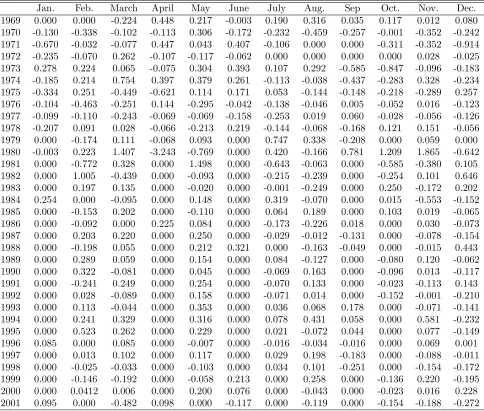
Table 1: Monetary Policy Shocks Using One Policy Reaction Function for1969-2001 (in percentage points)

Table 2: Monetary Policy Shocks Using Two Separate Policy Reaction Functions for 1969-1979:2 and 1979:3-2001 (in percentage points)