Munich Personal RePEc Archive
Multi-Dimensional Games (MD-Games)
Ruiz Estrada, M.A.
University of Malaya
15 September 2009
Multi-Dimensional Games (MD-Games)
Mario Arturo Ruiz Estrada1
Faculty of Economics and Administration, University of Malaya, 50603 Kuala Lumpur, MALAYSIA
Email: [email protected]
Website: www.econonographication.com
Tel: +006012-6850293
Abstract. This paper introduces the concept of Multi-Dimensional games (MD-games) based on the application of an alternative mathematical and graphical modeling approach to study the game theory from a multi-dimensional perspective. In fact, the MD-Games request the application of the mega-space coordinate system to visualize a large number of games, players, strategies and pay-offs functions into the same graphical space.
Keywords: Econographicology, non-cooperative game and game theory. JEL: C70
1. Introduction
The MD-games is willing to analyze a large number of games, players, strategies and payoffs functions from a multi-dimensional perspective. The difference between non-cooperative games and MD-games is that the concept about equilibrium from non-cooperative games which is supported by “the proof of the existence in any game of at least one equilibrium point. Other results concern the geometrical structure of the set of equilibrium points of a game with a solution, the geometry of sub-solutions, and the existence of a symmetrical equilibrium point in a symmetric game” (Nash, 1950). But in the case of the MD-games not request any equilibrium point, because all games in our model always keep in a constant dynamic imbalance state (Ruiz, 2008).
We also assume that in the MD-games exist a large number dimensions and each dimension is fixed a game. Hence, each game is located in different dimensions and each dimension is moving under different speeds of time respectively, it is supported by the application of the Omnia Mobilis Assumption (Ruiz, Yap and Shyamala, 2007). Therefore, each game into the mega-space coordinate system shows that the behavior of players and the selection of optimal strategies depend on the dimension they are located. In fact, all players in different games, they are free to choose different strategies according to his dimension and timing framework by logical, natural, analytical, cooperative and non-cooperative conditions.
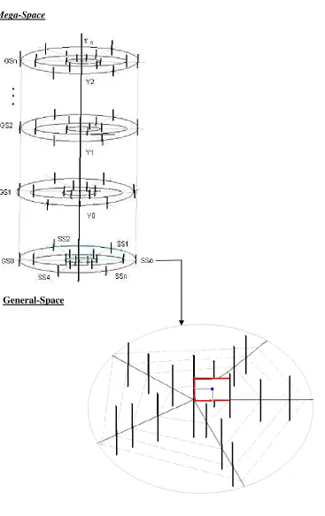
2. Introduction to The Mega-Space Coordinate System
(1.2.) m = [(X
<i:j:k:αh>),(Y
<i:j:k:βz>)]
Where i = { 1,2…∞ }; j = { 1,2…∞ }; k = { 1,2…∞ };L = { 1,2…∞ }; h = { 1,2…∞ } andz = { 1,2…∞ }
Therefore, the Mega-Space Coordinate System start from the General-Space 0 (See Expression 1.3.):
(1.3
.) U ≡ M = GS
0, SS
0:0, MS
0:0:0,
JI
[(X0:0:0:0),(Y0:0:0:0)])…
Until the General-Space infinity space ∞… (See expression 1.4.):
(1.4
.) GS
∞, SS
∞:∞, MS
∞:∞:∞, JI
[(X∞:∞:∞:∞),(Y∞:∞:∞:∞)])…∞
However, the final general function to analyze the Mega-Space Coordinate system is equal to expression 1.5. and 1.6.:
(1.5.)
M = ƒ (GS
i, SS
i:j, MS
i:j:k,
JI
m)
Where h = { 1,2…∞ }; z = { 1,2…∞ } and L = { 1,2…∞ }
(1.6.)
m= [(X
<i:j:k:αh>),(Y
<i:j:k:βz>)]
Where i = { 1,2…∞ }; j = { 1,2…∞ };h = { 1,2…∞ } and z = { 1,2…∞ }
3. Definition of Time in the Mega-Space Coordinate System
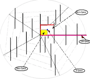
The basic premise of this research paper is that the Mega-Space or Universe is Multi-dimensional. This premise is supported by the second assumption where the Mega-space is running on a general time, but in the case of General-Spaces, Sub-Spaces, Micro-Spaces (See Figure 2) are running in partial times simultaneously. Finally, the JI-spaces are running in constant times. The JI-Space is a rigid body (or a value) that just hanging into its Micro-Space respectively. When we join all JI-Spaces together can generate a linear curve or non-linear curves into its Micro-Space. The Mega-space coordinate system applied three different types of time into its graphical modeling, these types of times are the general time (wt), partial times (wp) and constant times (wk) (See Expressions 2.1. and 2.2)
(2.1.)
Mwt
= ƒ (GS
i/wp , SSi:j/wp , MSi:j:k/wp , JIm/wk)Where h = { 1,2…∞ } and z = { 1,2…∞ }
(2.2.)
m
wk= [(X
<i/wp: j/wp: k/wp: αh/wk>),(Y
<i/wp: j/wp:k/wp :βz/wk>)]
FIGURE 1:
Mega-Space Coordinate System
Mega-Space
FIGURE 2:
General-Space, Sub-Space, Micro-Space and JI-Space
General-Space
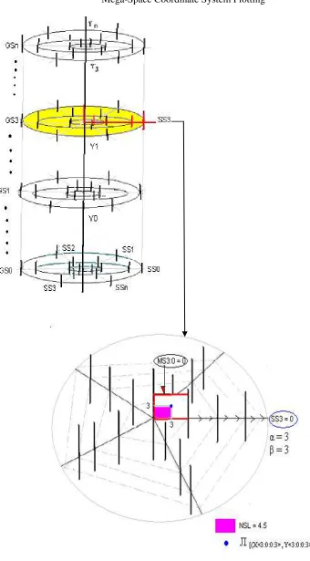
4. How to plot on the Mega-space Coordinate System
The Mega-Space Coordinate system plotting request four basic steps, there are follow by:
First Step: We need to choose our General-Space (GSi) from the Mega-space coordinate system, in our
case we decide to use the General Space on the third level (GS3).
Second Step: We proceed to choose our Sub-Space (SSi:j) from the General Space on the third level GS3.
Finally, we choose the Sub-Space 0 (SS3:0).
Third Step: Our Micro-Space (MSi:j:k) is originated from the General-Space third level GS3 , Sub-Space 0
(SS3:0) and Micro-space 0 (MS3:0:0).
Fourth Step: Finally, we start to plot our JI-Space into the Micro-Space 0 (MS3:0:0). In our case the
FIGURE 3:
Mega-Space Coordinate System Plotting
5. The Multi-Dimensional Games (MD-Games)
According to the MD-Games, it is based on the application of five basic theorems, there are follow by:
Theorem 1:
We have a large number of Games (
G), each game is
located on different market level (i) with different number of players (j), strategies (n) and payoffs functions (JI) (See Expression 4.1.). A basic premise in the MD-games is that each game has its specific dimension into the mega-space coordinate system, at the same time, all players (j) are taking different speed of time (☼) to choose its strategy (See Expression 4.2.). Moreover, all players (j) have the freedom to choose any strategy (n) anytime and anywhere, but always exists the high possibility to have a coalition in some games (spaces or dimensions) simultaneously into the mega-space coordinate system.(4.1.)
G
i:j:n:JI(4.2.) j=ƒ(☼n)
i= {0,1,2,3…∞}; j = {0,1,2,3…∞}; d = {0,1,2,3…∞}; n= {0,1,2,3…∞}; JI= {0,1,2,3…∞}
Theorem 2:
All players (j) are exchanging asymmetric or symmetric information in real time (╬). Therefore, the
MD-Games don’t need a single equilibrium point, because all games and players decisions depend on a dynamic imbalance state. In fact, the MD-Games suggest the application of the Omnia Mobilis assumption for the relaxation of all games, player and strategies into each dimension in the mega-space coordinate system respectively (See Expression 4.3.).
(4.3.)
☼
G
i:j:n:JI╬
……..╬
☼
G
i:j:n:JITheorem 3:
The decisions to choose any strategy (n) by any player (j) depend on natural conditions (S1k) or vulnerability conditions (S2K) or high risk conditions (S3K) (See Expression 4.4.).
(4.4.) n
= ƒ(S
1:k:S
2:K:S
3:K) Where
k = {0,1,2,3…∞}Theorem 4:
On the other hand, each game works under the application of informal negotiation (NIi) and formal
negotiation (Nf) in all games and players simultaneously (See Expression 4.5.). (4.5.)
∞ ☼
∫
Nf(α)n+1 i= 0╬
Gi:j:n:JI
∞ ☼
∫
NI(β)n+1j= 0
Hence, the final solution of the payoff (Sf) in different game by different player can show two possible scenarios: winner player [☼S*] or loser player [☼-S*]. Itis according to the final optimal game solution (See Expression 4.6.)
(4.6.) [☼S*] <☼Sf > [☼-S*]
Theorem 5:
The payoffs of each player (PO) can be positive or negative, it is according to the optimal game solution (S*max) or non-optimal game solution (-S*min) can get into the final process of negotiation (See Expression 4.7.).
(4.7.) S*max≈ PO ≈ -S*min
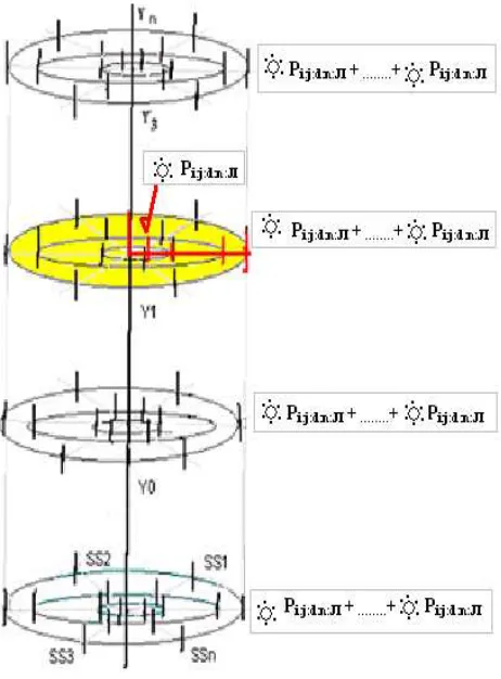
[image:8.612.237.468.332.645.2]Finally, we can observe that on the mega-space coordinate system a large number of games, players, strategies and payoffs functions are interacting together into the same graphical space (See Figure 4).
FIGURE 4:
6. Conclusion
In the case of infinity game under the application of the Multi-Dimensional games, this model
not requests any equilibrium point such as a finite game under non-cooperative game always
request. According to the MD-games, all games and players always keep in permanent dynamic
imbalance state.
7. References