http://dx.doi.org/10.4236/aces.2016.63024
An Accurate and Computationally Efficient
Explicit Friction Factor Model
Uchechukwu Herbert Offor, Sunday Boladale Alabi
Department of Chemical and Petroleum Engineering, University of Uyo, Uyo, Nigeria
Received 23 March 2016; accepted 30 March 2016; published 24 May 2016
Copyright © 2016 by authors and Scientific Research Publishing Inc.
This work is licensed under the Creative Commons Attribution International License (CC BY). http://creativecommons.org/licenses/by/4.0/
Abstract
The implicit Colebrook equation has been the standard for estimating pipe friction factor in a fully developed turbulent regime. Several alternative explicit models to the Colebrook equation have been proposed. To date, most of the accurate explicit models have been those with three logarith-mic functions, but they require more computational time than the Colebrook equation. In this study, a new explicit non-linear regression model which has only two logarithmic functions is de-veloped. The new model, when compared with the existing extremely accurate models, gives rise to the least average and maximum relative errors of 0.0025% and 0.0664%, respectively. Moreo-ver, it requires far less computational time than the Colebrook equation. It is therefore concluded that the new explicit model provides a good trade-off between accuracy and relative computation-al efficiency for pipe friction factor estimation in the fully developed turbulent flow regime.
Keywords
Colebrook Equation, Explicit Models, Computational Time, Friction Factor, Complexity
1. Introduction
Friction factor estimation is important for modeling flows in pipes and is relevant in most engineering discip-lines, for example: chemical, civil and mechanical. Over the years, the Colebrook equation [1][2] has been widely used for pipe friction factor estimation in the fully developed turbulent regime. The equation is expressed as:
1 2.51
2 log
3.71 Re
D
f f
ε
= − +
(1)
it-eration to obtain its solution. For simulations of long pipes and network of pipes, the Colebrook equation must be solved a huge number of times [3]. Therefore, an iterative solution to the Colebrook equation will be time consuming. The use of the Moodychart [4], as an alternative to the Colebrook equation, eliminates the require-ment for iteration. However, it is a graphical tool and therefore not convenient for computer-based simulations. The quest for a fast, non-iterative and accurate model, as an alternative to the Colebrook equation, has given rise to various explicit friction factor models. These explicit models differ in their accuracies and relative computa-tional efficiencies, depending on their degree of complexity.
In this work, a new explicit model was developed for estimating friction factor in the range for which the Co-lebrook equation is valid. The trade-off between model accuracy and relative computational efficiency has been considered.
The remaining sections of this paper are organized as follows: Section 2 reviews the available explicit friction factor models based on accuracy, complexity and relative computational efficiency. In Section 3, the develop-ment of the proposed model is presented while Section 4 reports the performance of the proposed model in comparison with those of the selected existing explicit models. In the final section, relevant conclusions are drawn based on the results obtained in this study.
2. Review of the Explicit Forms of the Colebrook Equation
2.1. Accuracy
The accuracies of the existing explicit models have been reported using common criteria such as the mean square error (MSE), percentage relative error and absolute error [5]-[8]. Model selection criteria (MSC) and Akaike information criterion (AIC) were used by Romeo, Royo and Monzon [9] for explicit model selection. These criteria were subsequently used by Genić et al. [7] and Yildrim [8] for comparison of several explicit models. Unfortunately, there is an apparent discrepancy in the MSC values reported [7][9] for the same models. For example, the MSC values reported by Romeo, Royo and Monzon [9]and Genić et al. [7] for Moody [10]
and Chen [11] models showed a wide contrast.
It has been shown that models with greater number of logarithmic functions are generally more accurate than those with lesser number of logarithmic functions, although the former require more computational time than the latter [6]. For instance, it is observed from works of Brkić [12], Winning and Coole [6] and Fang, Xu and Zhou
[13], that the most accurate approximations are those by Zigrang and Sylvester [14], Serghides [15], Romeo, Royo and Monzon [9] and Buzzelli [16]. These models, with the exception of the model by Buzzelli [16], have three logarithmic functions (either natural logarithm or logarithm to base ten).
Brkić [12], based on maximum relative error criterion, classified the existing explicit models as extremely accurate (error ≤ 0.14%), very accurate (error up to 0.5%), moderately accurate (error up to 1.5%), less accurate (error up to 5%), non advisable (error up to 25%) and extremely inaccurate (error ≥ 80%). Based on this classi-fication, the performances of several explicit models were evaluated and their accuracies are summarized in Ta-ble 1. Yildrim [8] conducted a comparative review of 16 explicit models. In his work, friction factor data were generated by digitizing the Moody chart. The turbulent portion of the Moody chart is a graphical solution of the Colebrook equation. Hence, digitizing the Moody chart [4] may have introduced secondary errors in the overall analysis [12]. This view is supported by the error margin observed by Fang, Xu and Zhou [13]. Ghanbari, Far-shad and Rieke [17] also digitized the Moody chart [4] when developing their model. They claim that the model is valid for Reynolds number (Re) between 2100 ≤ Re ≤ 108. It is not obvious how data was obtained for Rey-nolds number between 2100 and 3000 (critical zone), since the Moody chart does not contain Re values in this range.
2.2. Model Complexity and Computational Efficiency
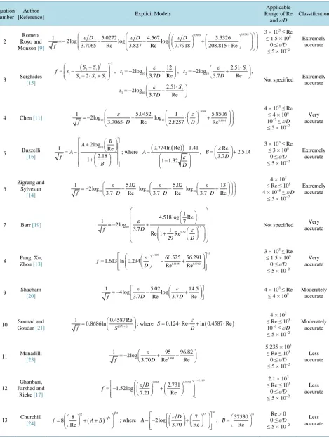
Table 1. Existing explicit friction factor models.
Equation Number
Author
[Reference] Explicit Models
Applicable Range of Re
and ε/D
Classification
2
Romeo, Royo and Monzon [9]
0.9345 0.9924
7.7
1 5.0272 4.567 5.3326
2 log log log
3.7065 Re 3.827 Re 9 81 208.815 Re
D D D
f
ε ε ε
= − − − + +
3 × 10³ ≤ Re
≤ 1.5 × 10⁸
0 ≤ ε/D ≤ 5 × 10⁻²
Extremely accurate
3 Serghides [15]
( )2 2
2 1 1
3 2 2 1 S S
f s
S S S
−
−
= −
− ⋅ +
, 1 10
12 2log 3.7 Re s D ε = − + , 1 2 10 2.51 2log 3.7 Re S s D ε ⋅ = − + , 2 3 10 2.51 2log 3.7 Re S s D ε ⋅ = − +
Not specified Extremely accurate
4 Chen [11]
1.1098
10 10 0.8981
1 5.0452 1 5.8506
2log log
3.7065 D Re 2.8257 D Re
f ε ε = − ⋅ − ⋅ ⋅ +
4 × 10³ ≤ Re
≤ 4 × 10⁸
10−7 ≤ ε/D ≤ 5 × 10⁻²
Very accurate
5 Buzzelli [16] 10 2log 1 Re 2.18 1 B A A f B + = − +
; where
(
0.774ln Re( ))
1.411 1.32 A D ε − − +
, Re 2.51 3.7D B ε + A
=
3 × 10³ ≤ Re
≤ 3 × 10⁸
0 ≤ ε/D ≤ 5 × 10⁻²
Extremely accurate 6 Zigrang and Sylvester [14]
10 10 10
1 5.02 5.02 13
2log log log
3.7 D Re 3.7 D Re 3.7 D Re
f
ε ε ε
= − ⋅ − ⋅ ⋅ − ⋅ ⋅ +
4 × 10³
≤ Re ≤ 108
4 × 10⁻⁵ ≤ ε/D ≤ 5 × 10⁻²
Extremely accurate
7 Barr [19] 0.7
0 10
.52 1 e 1 Re
29 1 4.518 log Re
1 7 2 log 3.7 R D D f ε ε + = − +
Not specified Very accurate
8 Fang, Xu, Zhou [13]
2 1.1007
1.1105 1.0712 60.525 56.291 1.613 ln 0.234
Re Re f D ε − = − +
3 × 10³ ≤ Re
≤ 1.5 × 10⁸
0 ≤ ε/D ≤ 5 × 10⁻²
Very accurate
9 Shacham [20]
1 5.02 14.5
4log log
3.7D Re 3.7D Re
f ε ε = − − +
4 × 10³ ≤ Re
≤ 4 × 10⁸
Moderately accurate
10 Sonnad and
Goudar [21] ( 1)
1 0.4587 Re 0.8686ln S S
S
f +
=
; where S 0.124 ReD ln 0.4587 Re( ) ε
= ⋅ ⋅ + ⋅
4 × 10³
≤ Re ≤ 108
10−6 ≤ ε/D ≤ 5 × 10⁻²
Moderately accurate
11 Manadilli
[23] 0.983
1 95 96.82
2log
3.70D Re Re
f
ε
= − + −
5.235 × 10³
≤ Re ≤ 108
0 ≤ ε/D ≤ 5 × 10⁻²
Less accurate
12
Ghanbari, Farshad and
Rieke [17]
2.169 1.042 0.9152 2.731 1.52log 7.21 Re D f ε − = − +
2.1 × 10³
≤ Re ≤ 108
0 ≤ ε/D ≤ 5 × 10⁻²
Less accurate
13 Churchill
[24] ( )
1 12 12 3 2 8 8 Re
f = + A+B−
; where
16 0.9 7 2log
3.70 Re
A − ε D +
= , 16 37530 Re
B=
Re > 0 0 ≤ ε/D ≤ 5 × 10⁻²
Continued
14 Round [25] 1 1.8log Re( )
0.135 Re D 6.5
f ε
= ⋅ ⋅ +
4 × 10³
≤ Re ≤ 108
0 ≤ ε/D ≤ 5 × 10⁻²
Non-advisable
15 Brkić [26]
0.4343 1
2log 10
3.71D f
β ε
− ⋅
= − +
where
(
)
Re ln
1.1 Re 1.816 ln
ln 1 1.1 Re β =
⋅
⋅ + ⋅
Not specified Less accurate
16 Rao and Kumar [27]
( )1
10 2 1
2log
0.444 0.135Re Re
D
f
ε
β
−
= +
where
2
Re 0.33 ln
6.5
1 0.55e
β −
= − Not specified Extremely inaccurate
17 Swamee and Jain [28]
1.11
10 0.9
1 5.74
2log
3.7D Re
f
ε
= − +
5 × 10³
≤ Re ≤ 108
10−6≤ ε/D ≤ 5 × 10⁻²
Less accurate
18
Vantankhah and Kouchakzadeh
[29] ( )
0.9633
1 0.4587 Re
0.8686ln
0.31G G
f G +
=
−
where G=0.124Re
(
ε D)
+ln 0.4587 Re(
)
5 × 10³
≤ Re ≤ 108
10−6 ≤ ε/D ≤ 5 × 10⁻²
Extremely accurate
more complex than the models which have two and less internal iterations
Winning and Coole [6] carried out a comparative review of 28 explicit friction factor models. They defined relative computational efficiency as the time taken by an explicit model to perform a task relative to the time taken by the Colebrook equation. The use of computational efficiency in their work clearly showed the impact of model complexity on the simulation time. They found that the models developed by Buzzelli [16] and Serg-hides [15] were the most accurate when ordered by absolute and relative errors, but when ordered by relative computational efficiencies, they ranked very low. The overall ranking reported was biased since it is not based on actual values of accuracy and relative computational efficiency. It was based on the number of available ex-plicit models. If this number is altered, the values of the combined ranking may change.
Computational efficiency is observed to be dependent on the type of logarithmic function(s) contained in the reported models. The computation of the logarithm function in many computer languages is based on series ex-pansion that requires several powers of arguments to be computed and added to each other [18]. Glustolisi [18]
and co-worker state that the natural logarithm function executes faster than the logarithmic function to base ten. This is based on the fact that the convergence function used for its computation is quite fast. Therefore, the computation of the logarithm function to base ten in many computer languages is based on the computation of the natural logarithm [18]. It should be noted that an explicit equation which requires computational time longer than that of the Colebrook’s equation defeats the aim of its development. An ideal explicit model should give a good trade-off between its accuracy and relative computational efficiency.
3. The Proposed Nonlinear Model
3.1. Data Generation
Using Microsoft Excel spread sheet, friction factor (f)data within an error limit of 10−9 were obtained from Eq-uation (1) for Re values in the range 4 × 10³≤ Re ≤ 108, using 1000 intervals in geometric order and (ε/D) value ranging from 10−6 to 0.05 using 28 intervals in arithmetic order. Thus, producing a matrix of 28,000 datasets for
f, Re and (ε/D) was obtained for model.
3.2. Model Development
function was introduced to enhance the computational efficiency of the model as noted by Glustolisi [18]. After some rearrangements, the proposed new model was thus obtained as:
10
2 log ln
Re Re
h d
b D e
D f
a c g
ε ε
= − + +
+
(19)
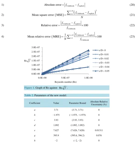
Using surface-fitting function in the MATLAB curve-fitting toolbox, coefficients a, b, c, d, e, g,and h with their parameter bounds were obtained at 95% confidence level (Table 2). The uncertainties associated with the esti-mated parameters, which are a measure of the reliability of the parameters, and consequently, a measure of the adequacy of the model, are reported in Table 2. A model which has parameter estimates with low levels of un-certainties (narrow intervals) is deemed to be good and adequate [30].
3.3. Performance Criteria
1) Absolute error= fColebrook−fexplicit (20)
2)
(
)
(
)
2
Colebrook explicit 1
Mean square error MSE
i N
i f f
N
=
= −
=
∑
(21)3) Colebrook explicit
Colebrook
Relative error f f 100
f
−
×
= (22)
4)
(
)
1 Colebrook explicitColebrook
Mean relative error MRE 1 i Ni f f 1 00
N f
= =
−
×
[image:5.595.92.539.243.714.2]=
∑
(23) [image:5.595.172.457.567.719.2]Figure 1. Graph of Re against Re f .
Table 2. Parameters of the new model.
Coefficient Value Parameter Bound Absolute Relative Uncertainty (%)
a 3.71 (3.71, 3.71) 0
b −1.975 (−1.975, −1.975) 0
c 3.93 (3.93, 3.93) 0
d 1.092 (1.092, 1.092) 0
e 7.627 (7.626, 7.628) 0.01311
g 395.9 (395.6, 396.2) 0.076
h −2 (−2, −2) 0
0.0E+00 5.0E+06 1.0E+07 1.5E+07 2.0E+07 2.5E+07 3.0E+07
0.0E+00 5.0E+07 1.0E+08
Reynolds number (Re)
e/D= 0
e/D= 0.01 e/D= 0.02
e/D = 0.03
e/D = 0.04 e/D = 0.05
5) Relative Computational efficiency: According to Winning and Coole [6], relative computational efficiency is the ratio of the time required by the explicit model to perform a task to the time required by the Colebrook equation to perform the same task. It means that a model with relative computational efficiency value greater than one (1.0) will require more time than the Colebrook equation to perform a particular task and vice-versa for a model with a value less than one (1.0).
Ten million friction factor calculations were performed using the available explicit models in the ranges of Re and
ε
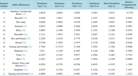
D for which the Colebrook equation is valid. These calculations were performed four times and the av-erage was recorded for each of the explicit model. For this analysis, f values for the Colebrook equation were determined using the method developed by Clamond [3] because of its speed of convergence. The relative computational efficiency was thereafter determined based on the approach proposed by Winning and Coole [6]. The results are as shown in Table 4.3.4. Model Accuracy, Adequacy and Computational Efficiency
It is observed from Table 3 that the new model (for this study), having the least mean relative and maximum relative errors of 0.0025% and 0.0664%, respectively, is more accurate than the selected extremely accurate models. In addition to the high accuracy of the new model from this study, its parameters are observed to have very low uncertainties ≤ 0.076% (see Table 2). This indicates that the parameters are known precisely. Conse-quently, the model is deemed very accurate and adequate for predicting friction factor.
It is observed from Table 4 that all the existing extremely accurate models, with the exception of Buzzelli [16]
equation, have relative computational efficiencies greater than one (1.0). This is not unexpected, given their complexity with respect to the number of logarithmic functions contained in the models. On the contrary, rela-tive computational efficiency values of less than one have been reported in the work of Winning and Coole [6]
for all the extremely accurate models. These values are disputable considering the complexity of these models (in terms of the numbers of logarithmic functions). Our findings show that the Buzzelli [16] model is almost two times faster than the Serghides [15], Romeo, Royo and Monzon [9], Zigrang and Sylvester [14] models. The Buzzelli [16] model has only two logarithmic functions, a combination of logarithm to base ten and the natural logarithm functions. The Buzzelli’s [16] model, based on the analysis in this study, is the best existing model in terms of accuracy and relative computational efficiency. However, it is found that that the new model is 39 and 1.9 times (in terms of mean and maximum relative errors, respectively) more accurate than the Buzzelli [16]
[image:6.595.87.538.499.694.2]model (see Table 3). Interestingly, the new model has two logarithmic functions and a higher accuracy (see
Figure 2 for error distribution). It has approximately the same relative computational efficiency as the Buzzelli
[16] model, which has only two logarithmic functions. Thus, the new model is regarded as a superior model to the existing extremely accurate explicit models.
Table 3. Explicit models ordered by maximum relative error.
Equation
number Reference
Absolute Error
MSE
Percentage Relative Error (%)
Minimum Maximum Average Minimum Maximum Mean
19 This study 3.176E−12 2.306E−05 7.868E−07 4.662E−12 6.730E−09 0.0664 0.0025
2 Serghides [15] 6.465E−08 8.965E−05 5.377E−05 3.446E−09 1.620E−04 0.1255 0.0978
3 Buzzelli [16] 9.740E−13 8.977E−05 5.438E−05 3.511E−09 9.544E−09 0.1255 0.0990
4 Zigrang and Sylvester [14] 3.152E−08 8.965E−05 5.444E−05 3.474E−09 8.454E−05 0.1255 0.1011
18 Vantankhah and
Kouchakzadeh [29] 7.882E−11 9.517e−05 2.158E−05 9.836e−10 2.625E−07 0.1332 0.0614
5 Romeo, Royo and
Monzon [9] 3.692E−06 6.382E−05 2.449E−05 7.188E−10 2.490E−02 0.1462 0.0477 6 Chen [11] 2.858E−08 1.258E−04 3.456E−05 1.743E−09 1.029E−04 0.3596 0.0709
7 Barr [19] 1.047e−09 3.281E−04 5.207E−05 5.010E−09 2.387E−06 0.5089 0.0942
8 Fang, Xu, Zhou [13] 3.101E−08 4.612E−04 8.178E−05 1.095E−08 7.320E−05 0.5997 0.1645
9 Shacham [20] 2.044E−09 3.464E−04 5.659E−05 4.034E−09 6.200E−06 0.8679 0.1254
10 Sonnad and Goudar [21] 6.593E−06 3.961E−04 8.527E−05 1.093E−08 7.413E−02 0.9926 0.1697
11 Haaland [22] 9.660E−09 7.309E−04 1.713E−04 3.736E−08 2.128E−05 1.2910 0.3241
12 Manadilli [23] 6.261E−09 1.863E−03 2.898E−04 2.159E−07 1.945E−05 2.5827 0.5485
13 Ghanbari, Farshad
and Rieke [17] 1.740E−09 2.000E−03 2.657E−04 2.121E−07 1.399E−04 2.7744 0.7810
16 Brkić [26] 5.781E−07 2.178E−03 2.854E−04 2.733E−07 8.089E−04 2.9427 0.5403
14 Churchill [24] 1.529E−07 2.025E−03 3.019E−04 2.864E−07 1.518E−03 3.2178 0.5746
18 Swamee and Jain [28] 1.254E−07 2.479E−03 3.333E−04 3.159E−07 1.271E−03 3.436 0.6300
15 Round [25] 1.551E−08 6.000E−03 2.600E−03 1.033E−05 2.219E−04 8.3383 4.4466
17 Rao and Kumar [27] 5.631E−09 3.991E−02 1.480E−03 1.651E−05 1.195E−05 85.479 5.5086
Table 4. Computational efficiencies of the proposed and existing explicit models.
Equation
number Author [Reference]
Simulation time 1 (s)
Simulation time 2 (s)
Simulation time 3 (s)
Simulation time 4 (s)
Mean Simulation time (s)
Relative Computational
efficiency
13 Ghanbari, Farshad and
Rieke [17] 2.0018 2.0018 1.9825 2.1063 2.0231 0.3776 3 Buzzelli [16] 2.0160 1.9813 2.0708 2.1527 2.0552 0.3836
19 This study 2.0828 2.0082 2.0730 2.1669 2.0827 0.3883
11 Haaland [22] 2.0833 2.0080 2.2566 2.0259 2.0935 0.3907
16 Brkić [26] 2.0687 2.1409 2.1994 2.1103 2.1298 0.3974
12 Manadilli [23] 2.1511 1.9947 2.3941 2.0287 2.1421 0.3998
18 Rao and Kumar [27] 2.2285 2.4316 2.1779 2.0146 2.2131 0.4130
15 Round [25] 2.5790 2.1902 2.2479 2.1139 2.2828 0.4260
10 Sonnad and Goudar [21] 2.7362 2.71272 2.7368 2.7202 2.7264 0.5088
9 Shakham [20] 3.921 4.1258 4.1667 4.1146 4.082 0.7650
6 Chen [11] 4.3073 4.1367 3.9977 4.1984 4.1601 0.7763
7 Barr [19] 4.5447 4.2223 4.1907 4.3816 4.3348 0.8090
5 Romeo, Royo and
Monzon [9] 6.0524 6.2378 6.0786 6.0439 6.1032 1.1390
2 Serghides [15] 6.0707 6.1784 6.1017 6.1326 6.1334 1.1447
[image:7.595.58.539.457.720.2]4. Conclusion
A new explicit model is developed for predicting friction factor in the range for which the Colebrook equation is valid. Until now, the best predictions are obtained with models having three logarithmic functions. The new simple model having only two logarithmic functions and maximum relative error of 0.0664% in this study is found to be more accurate than the selected existing extremely accurate models. Moreover, the relative compu-tational efficiency (0.3883) of the new model is in close agreement with that (0.3836) of the Buzzelli [16] which was adjudged as the best existing model in this work. Therefore, the new model provides a good trade-off be-tween accuracy and relative computational efficiency. Thus it is superior model to the existing explicit models for estimating pipe friction factor in the fully developed turbulent flow regime.
Acknowledgements
The authors are grateful to Dr. James F. Whidborne, a Reader at the School of Aerospace, Transport and Manu-facturing, Cranfield University, United Kingdom, for his suggestions regarding the technical contents of this paper. Thanks to Emma Hughes, a Doctoral Candidate at La Trobe University, Australia, for proofreading this paper.
References
[1] Colebrook, C.F. (1939) Turbulent Flow in Pipes, with Particular Reference to the Transition Region between the Smooth and Rough Pipe Laws.Journal of the Institution of Civil Engineers, 11, 133-156.
http://dx.doi.org/10.1680/ijoti.1939.13150
[2] Colebrook, C.F. and White, C.M. (1937) Experiments with Fluid Friction Factor in Roughened Pipes. Proceedings of the Royal Society of London. Series A: Mathematical and Physical Sciences, 161, 367-381.
http://dx.doi.org/10.1098/rspa.1937.0150
[3] Clamond, D. (2009) Efficient Resolution of the Colebrook Equation. Industrial & Engineering Chemistry Research, 48, 3665-3671. http://dx.doi.org/10.1021/ie801626g
[4] Moody, L.F. (1944) Friction Factors for Pipe Flow. Transactions of the American Society of Mechanical Engi-neers, 66, 671-681.
[5] Zigrang, D.J. and Sylvester, N.D. (1985) A Review of Explicit Friction Factor Equations. Journal of Energy Resources Technology, 107, 280-283. http://dx.doi.org/10.1115/1.3231190
[6] Winning, H.K. and Coole, T. (2013) Explicit Friction Factor Accuracy and Computational Efficiency for Turbulent Flows in Pipes. Flow, Turbulence and Combustion, 90, 1-27.
[7] Genić, S., et al. (2011) A Review of Explicit Approximations of Colebrook’s Equation. FME Transactions, 39, 67-71.
[8] Yildirim, G. (2009) Computer-Based Analysis of explicit approximations to the Implicit Colebrook—White Equations in Turbulent Flow Friction Calculation. Advances in Engineering Software, 40, 1183-1190.
http://dx.doi.org/10.1016/j.advengsoft.2009.04.004
[9] Romeo, E., Royo, C. and Monzon, A. (2002) Improved Explicit Equation for Estimation of the Friction Factor in Rough and Smooth Pipes. Chemical Engineering Journal, 86, 369-374.
http://dx.doi.org/10.1016/S1385-8947(01)00254-6
[10] Moody, L.F. (1947) An Approximate Formula for Pipe Friction Factors. Trans ASME, 69, 1005-1011.
[11] Chen, N.H. (1979) An Explicit Equation for Friction Factors in Pipes. Industrial & Engineering Chemistry Funda-mentals, 18,296-297. http://dx.doi.org/10.1021/i160071a019
[12] Brkić, D. (2011) Review of Explicit Approximations to the Colebrook Relation for Flow Friction. Journal of Petro-leum Science and Engineering, 77, 34-48. http://dx.doi.org/10.1016/j.petrol.2011.02.006
[13] Fang, X., Xu, Y. and Zhou. Z. (2011) New Correlations of Single-Phase Friction Factor for Turbulent Pipe Flow and Evaluation of Existing Single-Phase Friction Factor Correlations. Nuclear Engineering and Design, 241, 897-902. http://dx.doi.org/10.1016/j.nucengdes.2010.12.019
[14] Zigrang, D.J. and Sylvester. N.D. (1982) Explicit Approximations to the Solution of Colebrook’s Friction Factor Equa-tion. AIChE Journal, 28, 514-515. http://dx.doi.org/10.1002/aic.690280323
[15] Buzzelli, D. (2008) Calculating Friction in One Step. Machine Design, 80, 54-55.
[16] Seghides, T.K. (1984) Estimate Friction Factor Accurately. Chemical Engineering Journal, 91, 63-64.
Assurance. Journal of Chemical Engineering and Materials Science, 2, 83-86.
[18] Glustolisi, O., Berardi, L. and Walski, T.M. (2011) Some Explicit Formulations of Colebrook-White Friction Factor Considering Accuracy vs. Computational Speed. Journal of Hydroinformatics, 13, 401-418.
http://dx.doi.org/10.2166/hydro.2010.098
[19] Barr, D.I.H. (1981) Solutions of the Colebrook-White Function for Resistance to Uniform Turbulent Flow. Proceed-ings of the Institution of Civil Engineers, Part 2, 71, 529-535.
[20] Schorle, B.J., Churchill, S.W. and Shacham, M. (1980) Comments on: “An Explicit Equation for Friction Factor in Pipe”. Industrial & Engineering Chemistry Fundamentals, 19, 228-229. http://dx.doi.org/10.1021/i160074a019
[21] Sonnad, J.R. and Goudar, C.T. (2006) Turbulent Flow Friction Factor Calculation Using a Mathematically Exact Al-ternative to the Colebrook-White Equation. Journal of Hydraulic Engineering, 132, 863-867.
http://dx.doi.org/10.1061/(ASCE)0733-9429(2006)132:8(863)
[22] Haaland, S.E. (1983) Simple and Explicit Formulas for the Friction Factor in Turbulent Pipe Flow. Journal of Fluids Engineering, 105, 89-90. http://dx.doi.org/10.1115/1.3240948
[23] Manadilli, G. (1997) Replace Implicit Equations with Signomial Functions. Chemical Engineering Journal, 104, 129-130.
[24] Churchill, S.W. (1977) Friction Factor Equations Spans All Fluid-Flow Regimes. Chemical Engineering Journal, 84, 91-92.
[25] Round, G.F. (1980) An Explicit Approximation for the Friction Factor-Reynolds Number Relation for Rough and Smooth Pipes. The Canadian Journal of Chemical Engineering, 58, 122-123.
http://dx.doi.org/10.1002/cjce.5450580119
[26] Brkić, D. (2011) New Explicit Correlations for Turbulent Flow Friction Factor. Nuclear Engineering and Design, 241, 4055-4059. http://dx.doi.org/10.1016/j.nucengdes.2011.07.042
[27] Rao, A.R. and Kumar, B. (2007) Friction Factor for Turbulent Pipe Flow. Division of Mechanical Sciences, Civil En-gineering Indian Institute of Science, Bangalore, ID Code 9587.
[28] Swamee, D.K. and Jain, A.K. (1976) Explicit Equations for Pipe Flow Problems. Journal of the Hydraulics Division, 102, 657-664.
[29] Vantankhah, A.R. and Kouchakzadeh, S. (2008) Discussion of “Turbulent Flow Friction Factor Calculation Using a Mathematically Exact Alternative to Colebrook-White Equation” by Jagadeesh R. Sonnad and Chetan T. Goudar. Journal of Hydraulic Engineering, 134, 1187. http://dx.doi.org/10.1061/(ASCE)0733-9429(2008)134:8(1187)
[30] Motulsky, H.J. and Christopoulos, A. (2003) Fitting Models to Biological Data Using Linear and Nonlinear Regression: A Practical Guide to Curve Fitting. GraphPad Software Inc., San Diego.
Nomenclature
f Darcy friction factor [dimensionless]
D Internal pipe diameter [m]
ε Pipe absolute roughness [m]
ε/D Relative roughness (dimensionless) Re Reynolds number (dimensionless)
a-h The new model parameters (Equation (19))
![Figure 2 for error distribution). It has approximately the same relative computational efficiency as the Buzzelli [16] model, which has only two logarithmic functions](https://thumb-us.123doks.com/thumbv2/123dok_us/7932483.749487/6.595.87.538.499.694/distribution-approximately-relative-computational-efficiency-buzzelli-logarithmic-functions.webp)