4 Tier Neural Network based Model for Reliable

(1)

4-Tier Neural Network based Model for Reliable WSNs

Mamta Katiyar

ECE Department M. M. Engineering College,

M. M. University Mullana, Ambala, Haryana,

India-133207

H.P. Sinha,

Ph.D.

ECE Department M. M. Engineering College,

M. M. University Mullana, Ambala, Haryana,

India-133207

Dushyant Gupta,

Ph.D.

Electronics Department, University College,

KUK

Kurukshetra, Haryana, India-13611

ABSTRACT

Fault tolerance is one of the attractive inherent features of neural networks. This feature facilitates to retrieve the information of interest despite of corrupted signal in presence of faults in the network. This paper presents a reliable and fault tolerant model for reliable transportation of information in Wireless Sensor Networks. Work presented in this chapter is an attempt to make the senor nodes intelligent enough to deliver the information of interest to the base station despite of the fact that wireless communication medium is noisy and information may be corrupted during transportation. Algorithm supporting the functionality of the proposed model has been analyzed through the example.

Keywords

ANN, BAM, NN, WSN.

1. INTRODUCTION

A Neural Network (NN) is a system consisting of processing components called neurons connected in parallel or distributed manner in a graph topology. In NN, neurons are connected with each other through weights called synaptic strength of connections. Weights connect the network input layer to output layer. Knowledge of NN is stored in its connections and there is no requirement of any additional storage. One of the difficulties with NNs is choosing of appropriate topology for the problem. Different methods for training the neural networks are inspired from biology science which determines the way NNs learn. In all most all of these networks, training is based on learning by example. In the problem definition, set of samples defining the correct input-output data are often given to the network and using these examples, the network weights are adjusted accordingly to produce the desired output for respective input patterns. The most important feature of a NN is its ability to recognize the data affected by noise or intentional change and to remove those variations after training.

Neural networks are efficiently used in WSNs for optimal use of energy of sensor nodes. Requirements of WSNs can be easily satisfied by the algorithms developed in neural network in application areas like parallel distributed computation, distributed storage, data robustness, fault tolerance and low computation. In a WSN platform, neural networks can help through dimensionality reduction, obtained simply from the outputs of the neural networks clustering algorithms, leads to lower communication cost and energy savings [1]. The other reason to use neural network based methods in WSNs is the similarity in the behaviour of WSNs and ANNs. Authors in [2] shown that ANNs exhibit exactly the same architecture as WSNs where behaviour of neurons is similar to sensor nodes

and connections correspond to radio links. With this opinion, the whole sensor network can be seen as a neural network and within each sensor node inside the WSN.

2. ISSUES

In WSN, a packet may not be successfully transmitted to the destination because of the following reasons: (a) Probable forwarders inside the coverage are in good working condition but have not received the packet correctly because of noise etc. and (b) All the forwarders are in failure condition.

Our proposed model is an attempt to still improve the fault tolerance and reliability of packet delivery process in WSN. This model addresses the first reason of unsuccessful packet delivery in WSNs. Proposed model is well suited for the applications where the events that can occur in the network are from a predefined set of events. Assume that sensor node has to sense an event to receive a packet from a predefined set P = {p1, p2, p3, p4, p5, …,}; where the size of each packet is m-bit.

Larger is the size of a packet, more will be the chances of faulty delivery of packet to the next probable forwarder/destination because of noise etc. Authors in [3] shown that if a packet is compressed before transmission, we can take the advantage of compression ratio but the price one may have to pay will be distortion ratio.

Our proposed model is based on encoding the associations using neural network. For each message (packet) sensed by a sensor node, a small packet (vector) associated to the original packet is forwarded towards the destination as we know that transmitting an associated vector of small size has better reliability and fault tolerance.

Authors in [4][5][6][7] presented models where an input pattern is presented to a memory and then the corresponding output pattern is presented to the transpose memory. After that the output is feed the memory and so on, until a stable state is reached. Most of these models work with bipolar and binary patterns. These models (for example Bidirectional Associative Memory) are not able to guarantee the recall of all patterns.

3. SYSTEM MODEL

(2)

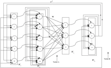
layer is applied on the weight matrix W between layer second and third to encode the association between the two

[image:2.595.58.532.94.385.2]

hetro associative vectors (signals) A and B where size of vector B is smaller than A.

Fig 1: Four Tier Network Structure for Improved Reliability / Fault Tolerance of Data Transportation in WSN

Encoded signal generated at third layer is applied to the Hopfield neural network at forth layer and it remains available at this layer until this encoded signal gets stabilized. Now finally this encoded signal is sent to the next forwarder for onwards transmission towards the sink.

Hopfield neural networks at the second and forth layers are used to improve the inherent fault tolerance of the network where partially corrupted pattern is recovered bit by bit to strengthen forward association A→B. Functionality of second and third layer together is same as of Bi-Directional Memory (BAM). The output of the second and forth layers is updated in asynchronous manner (i.e. one bit is updated at one time) and thus partially corrupted noisy signal is updated first and then it is sent to the subsequent layers for recalling the associated pattern.

3.1 Notations Used



 

 _i i

T i n

m A B

W * ( ) ( );

T n m T

m

n W

W* ( * )

. 0

1 ]

[

0 1 ]

[

* *

2

neuron layer subsequent in input as data

bit by bit copy to matrix Identity Otherwise

W

j i When W Where W W

Otherwise W

j i When W Where W W

ij ij n n ij I

ij ij m m ij Ii

      

   

ji ij ij

i i

T i m m ij H

W W and

j i When W Where A A W

Wi 

 

  

[ ]*



( )( ); 0

ji ij ij

i i

T i n n ij H

W W and

j i When W

Where B B W

W

  

  

[ ]*



( ) ( ); 0

2

Where ' i B , ' i

A are bipolar representation of vectors

A

iand

B

i

respectively and T i T

B) ( , )

(A' '

i are the transpose of vectors '

' i

A andBi.

3.2 Training Procedure

Activation functions used in the proposed 4-Tier neural network are as under:

A. For auto associative networks at layer second and forth:

0 ;

; 0

; 1 ) (

Out_j

 

  

j j

Net if output previous

negative is

Net if

positive is

Net if Net f

Where _ _



j j ji i OutW

a etj

N and ai is the ith bit of input

vector

B. For Bi-directional memory between 2 and layer-3

(Forward Association):

0 ;

; 0 ; 1 ) ( Out

 

  

negative is Net if

positive is Net if Net f

Net value is computed as under:

n m W A et . _*

N 

(3)



  

i

i T i n

m A B

W _* ( ) .( )

Forward Association:

Forward Association A→B is used at the source node sensing the event of interest.

Backward Association:

Backward association B→A is used at the base station to retrieve the actual event sent by the source node once encoded signal is received at the base station. Activation function used at the base station will be as under:

0 ;

; 0

; 1 ) ( Out A

 

  



negative is Net if

positive is Net if Net f

Where T

n m

W B

et .( )

N  * and

T n m

W )

( * is the transpose of

W

m*n.

3.3 Application Algorithm

Step1: Encode the associations for predefined event space:



 



i i T i n

m A B

W* ( ) . ; for forward associations in BAM

BAM in ns associatio backward

for ; . ) (



 



i i T i T

mXn B A

W

0 2

; . ) ( 1

 

  



ii i

i T i H

w Where layer

at network

e associativ auto

For A A W

0 4

; . ) (

2

 

 





ii i

i T i H

w Where layer

at

network e

associativ auto

For B B W

Step 2: Initialization of identity matrix to facilitate copy operation to the subsequent auto associative network layer.

n n I m m

I I andW I

W [ ] _* [ ]_*

2

1  

Step 3: Set the initial activation of layer-1 to the external input vector A.

A Out_layer_₁

While activation of the auto associative network at layer-2 are not converged do:

Step 4: Set the initial activation of layer-2 to the output of layer-1

i layer

i

A

I

a

Out

]

_



.



[

2

Step 5: Do steps 6-8 for each unit outi at layer-2

Step 6: Compute net input:



 

j

ji H j i

i a out W

net .[ ₁]

Step 7: Determine activation (output):

    

 



0 ;

; 0

; 1

]

[ ₂

i i

net if output previous

negative is net if

positive is net if

Out_i _layer _i

Step 8: Broadcast the value of [Outi]layer_₂to all other units

except itself.

Step 9: Test for convergence:

If auto associative network at layer-2 stabilized

then go to step 10;

else

go to step 5.

Step 10: Apply activation of layer-2 on the weight matrix W. Compute the net input at layer-3

W A W out

net[ ]layer2.  .

Step 11: Determine the activation (output) of layer-3.

    

 





0 ;

; 0

; 1

]

[ ₃

negative is

net if

positive is

net if

b Out_i _layer _i

Step 12: Set the initial activation of layer-4 to the output of layer-3.

[

out

_i

]

_layer4



B

.

I



b

_i

Step 13: Do steps 14-16 for each unit

4

]

[

Out

_i _layer_ .

Step 14: Compute net input:





  

j

ji H layer i i

layer

i b out W

net] [ ] .[ ]

[

2 4 4

Step 15: Determine the activation (output):

    

 



 

0 ] [ ; ] [ ; 0

] [ ; 1 ]

[

4 4

4

layer i layer

i layer i

layer i

positive is net if Out

B

Step 16: Broadcast the value of

[

Out

_i

]

_layer_₄to all other units except itself.

Step 17: Test for convergence:

If auto associative network at layer-4 stabilized then go to step 18;

else

go to step 13.

Step 18: Source node is ready to transmit the encoded signal to the next forwarder towards the base station.

At the base station, output of layer-4 is applied on T

W To recall the actual signal A.

    

 

0 ; ;

0 ; 1

) . ( ] [

positive is net if

W B f net f

A T

4. SYSTEM ANALYSIS

This section presents the analysis of proposed model to show the functionality and performance of WSN in presence of noise. As wireless communication medium is error prone, two reasons have been considered in this analysis for erroneous delivery of signal at the base station as under:

i. Error in the signal during the transmission due to mistaken bits (altered bits).

(4)

Functionality and performance of the proposed model has been illustrated through example as under considering bipolar representation of signals sensed by the sensor node (source node) for training the proposed neural network embedded in each sensor to differentiate between missing and mistaken bits and hence to differentiate between the two kind of errors during transmission in WSN. Analysis shows that proposed model has better fault tolerance for the transmission due to missing bits over the mistaken bits.

Example:

Consider the event space with the two samples A1 and A2 to

be sensed by the sensor nodes and to be sent to the base station in a WSN as under:

1]

0

1

0

1

0

1

0

1

0

1 [

1



A

0]

1

0

1

0

1

1 [

2



A

As we know that event smaller in size has better fault tolerance during transmission, we have associated vectors B1 and B2

respectively with events A1 and A2 for reliable data transfer

over the WSN. Associations are encoded and memorized in the connections (weights) of the neural network as under:

4.1.1 Encoding the Associations before

Transmission:

Input sample spaces associated vector for onward transmission 1] 0 0 1 0 1 1 0 0 1 1 0 1 0 0 1 [ 1

A B1[100111100]

0] 1 1 1 1 1 0 0 1 1 0 0 0 1 1 1 [ 2

A B2[111100111]

Bipolar versions: 1] 1 -1 -1 1 -1 1 1 -1 -1 1 1 -1 1 -1 -1 [

1

A ] 1 -1 -1 1 1 1 1 -1 -1 [

1

B 1] -1 1 1 1 1 1 -1 -1 1 1 -1 -1 -1 1 1 [

2

A B2[1111-1-1111]

Weight matrix  



 

i i T i n

m A B

W

W _* ( ) ( );

                                                                                     2 2 0 2 2 0 2 2 0 2 2 0 2 2 0 2 2 0 2 2 0 2 2 0 2 2 0 0 0 2 0 0 2 0 0 2 2 2 0 2 2 0 2 2 0 0 0 2 0 0 2 0 0 2 2 2 0 2 2 0 2 2 0 0 0 2 0 0 2 0 0 2 2 2 0 2 2 0 2 2 0 0 0 2 0 0 2 0 0 2 2 2 0 2 2 0 2 2 0 0 0 2 0 0 2 0 0 2 2 2 0 2 2 0 2 2 0 2 2 0 2 2 0 2 2 0 2 2 0 2 2 0 2 2 0 0 0 2 0 0 2 0 0 2 W



T n m T m n

W

_*

(

_*

)

                                                               2 2 2 0 2 0 2 0 2 0 2 0 2 2 2 0 2 2 2 0 2 0 2 0 2 0 2 0 2 2 2 0 0 0 0 2 0 2 0 2 0 2 0 2 0 0 0 2 2 2 2 0 2 0 2 0 2 0 2 0 2 2 2 0 2 2 2 0 2 0 2 0 2 0 2 0 2 2 2 0 0 0 0 2 0 2 0 2 0 2 0 2 0 0 0 2 2 2 2 0 2 0 2 0 2 0 2 0 2 2 2 0 2 2 2 0 2 0 2 0 2 0 2 0 2 2 2 0 0 0 0 2 0 2 0 2 0 2 0 2 0 0 0 2 W

0 );

(

)

(

]

[

*

2





i



i



ii



T i n

n ij

H

W

B

Where

W

                                                                                                                                1 1 1 1 1 1 1 1 1 1 1 1 1 1 1 1 1 1 1 1 1 1 1 1 1 1 1 1 1 1 1 1 1 1 1 1 1 1 1 1 1 1 1 1 1 1 1 1 1 1 1 1 1 1 1 1 1 1 1 1 1 1 1 1 1 1 1 1 1 1 1 1 1 1 1 1 1 1 1 1 1 1 1 1 1 1 1 1 1 1 1 1 1 1 1 1 1 1 1 1 1 1 1 1 1 1 1 1 1 1 1 1 1 1 1 1 1 1 1 1 1 1 1 1 1 1 1 1 1 1 1 1 1 1 1 1 1 1 1 1 1 1 1 1 1 1 1 1 1 1 1 1 1 1 1 1 1 1 1 1 1 1 2 H W                                              0 2 0 2 2 0 2 2 0 2 0 0 2 2 0 2 2 0 0 0 0 0 0 2 0 0 2 2 2 0 0 2 0 2 2 0 2 2 0 2 0 0 2 2 0 0 0 2 0 0 0 0 0 2 2 2 0 2 2 0 0 2 0 2 2 0 2 2 0 2 0 0 0 0 2 0 0 2 0 0 0 Similarly

0 );

(

)

(

]

[

*









i i ii

T i m

m ij

H

W

A

Where

W

i

4.1.2 Recalling the Actual Signal at the base

Station from Encoded Vector:

Case-1: No Error during the transmission of encoded signal from source to destination (base station)-

Consider that the event

1]

1 -1

-1

1 -1

1

1 -1

-1

1

1 -1

-1

[

1





A

is detected at the

sensor node (source node) for onward transmission to the base station. Before transmission, it is applied on weight matrix W and related associated pattern B1 is generated for onward

transmission as under:

Net at layer-3 = _*_W 1

A

= [+ive, -ive, -ive, +ive, +ive, +ive, +ive, -ive, -ive] Out at layer-3 = [1 0 0 1 1 1 1 0 0] = B1

When vector B1 is received at the base station, it is applied on

WT_{to generate original signal A}

1 as under:

Net= B1*WT= [+ive, -ive, -ive, +ive, -ive, +ive, +ive, -ive, -ive

+ive, +ive, -ive, +ive, -ive, -ive, +ive]

Out = [1 0 0 1 0 1 1 0 0 1 1 0 1 0 01]= A1 ; Actual signal

recalled.

Case-2: Error encounters during the transmission from source node to the destination (Base Station)-

(i) Fault tolerance of the proposed model in case error occurs due to mistaken bits:-

(5)

i.e. B1 = [-1 -1 -1 1 1 1 1 -1 -1].

Base station applies this vector on WT to retrieve the original signal associated with this received signal as under:

Net= B1 * WT

= [+ive, -ive, -ive, +ive, -ive, +ive, +ive, -ive, -ive +ive, +ive, -ive, +ive, -ive, -ive, +ive]

Out = [1 0 0 1 0 1 1 0 0 1 1 0 1 0 01] = A1; recall the original

signal.

Recovery of three bit fault: Consider that signal received at the base station (at layer-4 of neural network) encounters three faulty bits (first 3-digits as mistaken bit) during transmission.

i.e. B1 = [-11 1 1 1 1 1 -1 -1].

Net= B1 * WT

signal.

Recovery of four bit fault: Consider that signal received at the base station (at layer-4 of neural network) encounters 4-faulty bits (first 4-digits as mistaken bit) during transmission. i.e. B1 = [-11 1 -1 1 1 1 -1 -1].

Out # A1; failureto recover the original signal.

(ii). Fault tolerance of the proposed model in case error occurs due to missing bits:-

Recovery of three bit fault: Consider that signal received at the base station (at layer-4 of neural network) encounters three bit fault (2nd_{, 3}rd_{and 7}th_{digits are missing)}_during

transmission.

i.e. B1 = [1 0 0 1 1 1 0 -1 -1].

Net= B1 * WT

signal.

Recovery of four bit fault: Consider that signal received at the base station (at layer-4 of neural network) encounters four bit fault (2nd, 3rd, 7th and 8th digits are missing) during transmission.

i.e. B1 = [1 0 0 1 1 1 00 -1].

Net= B1 * WT

signal.

Recovery of five bit fault: Consider that signal received at the base station (at layer-4 of neural network) encounters five bit fault (2nd, 3rd , 7th ,8th and 9th digits are missing) during transmission.

i.e. B1 = [1 0 0 1 1 1 00 0 ].

Net= B1 * WT

signal.

Recovery of six bit fault: Consider that signal received at the base station (at layer-4 of neural network) encounters six bit fault (2nd_{, 3}rd _,6th_{, 7}th_,8th_{and 9}th_{digits are missing)}_during

transmission.

i.e. B1 = [1 0 0 1 1 0 0 0 0 ].

Net= B1 * WT

signal.

Recovery of seven bit fault: Consider that signal received at the base station (at layer-4 of neural network) encounters five bit fault (2nd, 3rd, 5th, 6th, 7th, 8th and 9th digits are missing)

during transmission.

i.e. B1 = [1 0 0 1 0 0 0 0 0 ].

Base station applies this vector on WT_{to retrieve the original}

signal associated with this received signal as under: Net= B1 * WT

Out # A1; failureto recover the original signal.

5. RESULTS AND DISCUSSION

(6)

6. REFERENCES

[1] A. Kulakov, D. Davcev, G. Trajkovski, “Application of wavelet neural-networks in wireless sensor networks”, Sixth International Conference on Software Engineering, Artificial Intelligence, Networking and Parallel/Distributed Computing and First ACIS International Workshop on Self-Assembling Wireless Networks (SNPD/SAWN'05), pp.262—267, 2005 [2] Oldewurtel, Frank, Mahonen, Petri, “Neural Wireless

Sensor Networks”, International Conference on systems & Networks Communications, ICSNS’06, pp. 28-28 .

[3] Vijay Kumar, R. B. Patel, Manpreet Singh and Rohit Vaid, “ A Neural Approach for Reliable and Fault Tolerant Wireless Sensor Networks”, in International Journal of Advanced Computer Science and Applications (IJACSA), Vol. 2(5), pp. 113-118, 2011.

[4] Y. F. Wang, “Guaranteed Record of all Training Pairs for Bidirectional Associative Memory ,” in IEEE Transactions on Neural Networks , vol. 1(6), pp. 559-567, 1991.

[5] L. Lee, W. J. Wangl, “Improvement of Bidirectional Associative Memories by using Correlation Significance”, in Electronics Letters, vol. 29(8), pp. 688-690, 1993.

[6] C. L. Leung, “Optimum Learning for Bidirectional Associative Memory in the sense of Capacity”, in IEEE Transaction on Systems, Man and Cybernetics, vol. 24(5), pp. 791-796, 1994.