Multi Valued Neuron with Sigmoid Activation Function for Pattern Classification

http://dx.doi.org/10.4236/jcc.2014.24023

Multi-Valued Neuron with Sigmoid

Activation Function for Pattern

Classification

Shen-Fu Wu, Yu-Shu Chiou, Shie-Jue Lee

Department of Electrical Engineering, National Sun Yat-sen University

Email: [email protected], [email protected], [email protected]

Received December 2013

Abstract

Multi-Valued Neuron (MVN) was proposed for pattern classification. It operates with complex-va- lued inputs, outputs, and weights, and its learning algorithm is based on error-correcting rule. The activation function of MVN is not differentiable. Therefore, we can not apply backpropagation when constructing multilayer structures. In this paper, we propose a new neuron model, MVN-sig, to simulate the mechanism of MVN with differentiable activation function. We expect MVN-sig to achieve higher performance than MVN. We run several classification benchmark datasets to com- pare the performance of MVN-sig with that of MVN. The experimental results show a good poten- tial to develop a multilayer networks based on MVN-sig.

Keywords

Pattern Classification; Multi-Valued Neuron (MVN); Differentiable Activation Function; Backpropagation

1. Introduction

The discrete multi-valued neuron (MVN) was proposed by N. Aizenberg and I. Aizenberg in [1] for pattern classification. The neuron operates with complex-valued inputs, outputs, and weights. Its inputs and outputs are mapped onto the complex plane. They are located on the unit circle, and are exactly the th

k roots of unity. The activation function of MVN k-valued logic maps a set of the th

k roots of unity on itself. Two discrete-valued MVN learning algorithms are presented in [2]. They are based on error-correcting learning rule and are deriva- tive-free. This makes MVN have higher functionality than sigmoidal or radial basis function neurons.

In this paper, we propose a new neuron model, MVN-sig, to simulate the mechanism of MVN with dif- ferentiable activation function. We consider the activation function of MVN as a function of the argument of a weighted sum. We stack multiple sigmoid functions to approximate this multiple step function. Hence, we can obtain a differentiable input/output mapping and we apply a naive gradient descent method as its learning rule. We expect MVN-sig to achieve better performance than MVN.

The rest of the paper is organized as follows. Section 2 briefly describes MVN and its activation function. Section 3 presents MVN-sig and the sigmoid activation function. The learning algorithm of MVN-sig is des- cribed in detail. Section 4 presents the results of three experiments. Finally, conclusions and discussions are given in Section 5.

2. Multi-Valued Neuron

2.1. Discrete MVN

A discrete-valued MVN is a function mapping from a n-feature input onto a single output. This mapping is described by a multiple-valued (k-valued) function of n-feature instances, f(x₁,,x_n), which uses n+1 complex-valued weights:

) (

= ) , ,

(x₁ x_n P _{0 1}x_{1 n}x_n

f  ω +ω ++ω (1) where x1, xn are the features of an instance, on which the performed function depends, and ω0, ω1, ωn

are the weights. The values of the function and of the features are complex. They are the kth roots of unity:

) / 2 (

=expi jk

j π

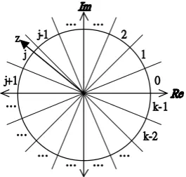
ε , j∈0,1,,k−1, and i is an imaginary unity. P is the activation function of the neuron:

k j z

arg k

j if k

j i z

P( )=exp( 2π ), 2π ≤ ( )< 2π( +1) (2)

where j=0,1,,k−1 are values of the k-valued logic, z=ω0+ω1x1++ωnxn is the weighted sum, and

) (z

arg is the argument of the complex number z. Equation (2) is illustrated in Figure 1.

Equation (2) divides the complex plane into k equal sectors and maps the whole complex plane onto a subset of points belonging to the unit circle. This subset corresponds exactly to a set of the _kth

roots of unity. The MVN learning is reduced to the movement along the unit circle and is derivative-free. The movement is determined by the error which is the difference between the desired and actual output. The error-correcting learning rule and the corresponding learning algorithm for the discrete-valued MVN were described in [5] and modified by I. Aizenberg and C. Moraga [3]:

, ) ( | | 1) ( = 1

i s q r r r

i r

i x

z n

C _{ε ε}

ω

ω −

+ +

+

(3)

for i=0,1,,n, where xi is the input of th

i feature with the components complex-conjugated, n is the number of the input features, εq is the desired output of the neuron, εs=P(z) is the actual output of the

neuron (see Figure 2), r is the number of the learning epoch, ωir is the current weighting of the th

i feature,

1 +

r i

ω is the following weighting of the ith feature after correction, Cr is the constant part of the learning rate

(it may always equal to 1), and |z_r| is the absolute value of the weighted sum obtained on the _rth

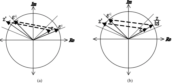
epoch. The factor

| |

1

r

z is useful when learning non-linear functions with a number of high irregular jumps. Equation (3) ensures that the corrected weighted sum moves from sector s to sector q (see Figure 2(a)). The direction of this movement is determined by the error δ =εq−εs. The convergence of the learning algorithm was proven in [6].

2.2. Continuous MVN

The activation function Equation (2) is piece-wise discontinuous. This function can be modified and generalized for the continuous case in the following way. When k→∞ in Equation (2), the angle value of the sector (see in Figure 1) will approach to zero. The activation function is transformed as follows:

| | = )) ( ( exp = ) (

z z z iarg z

P (4)

where z is the weighted sum, arg(z) is the argument of complex number z, and |z| is the modulus of the complex number z. The activation function Equation (4) maps the weighted sum into the whole unit circle (see Figure 2(b)). Equation (2) maps only to the discrete subsets of the points belonging to the unit circle. Equation (2) and Equation (4) are both not differentiable, but their differentiability is not required for MVN learning. The Learning rule of the continuous-valued MVN is shown as follows:

1_{= ( ) = ( ) ,}

( 1) | | ( 1) | | | |

r r r q s r r q

i i i i i

r r

C C z

x x

n z n z z

ω + ω ₊ ε ₋ε ω ₊ ε ₋

+ + (5)

for i=0,1,,n.

3. MVN with Sigmoid Activation Function

The learning algorithm of MVN is reduced to the movement along the unit circle on the complex plane. They are based on error-correcting learning rule and are derivative-free. Therefore, we can not use chain rule for error backpropagation to construct multilayer networks using MVN. In [3], I. Aizenberg and C. Moraga introduced a heuristic approach to construct the multilayer feedforward neural networks based on MVN. This inspired us to develop a differentiable activation function to which we can apply backpropagation learning rule. We expect the new learning rule to have more execution time but it can achieve better performance than MVN on a single neuron.

(a) (b)

3.1. Multi-Valued Sigmoid Activation Function

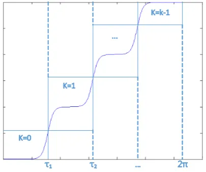
The basic idea of the multi-valued sigmoid activation function is to approximate the functionality of MVN using multiple sigmoid functions. In [7], E. Wilson presented a similar model for robot thruster control and farther applications. The original activation function of MVN is written in Equation (2). This activation function operates with the argument of weighted sum. Therefore, we can transfer this activation function into a function of argument which is illustrated in Figure 3. The corresponding MVN presentation is in Figure 4. This form of original activation function of MVN is a combination of multiple step functions, which can be approximated by stacking multiple sigmoid functions:

1 (₁ )

1 1

1 1 (₁ )

=1 =1

2 / ( ) =

1 exp

2 /

( ) = ( ) =

1 exp

i c _i

k k

i c _i

i i

k f

k

F f

θ τ

θ τ π

θ

π

θ θ

− −

− −

− −

+

+

∑

∑

where F(θ₁) is the multi-valued sigmoid activation function, θ1 is the argument of weighted sum, τi is the

argument of _ith

root of unity and f_i(θ₁) is the sigmoid function setting on τi. The activation function

2 1 1):

(θ θ →θ

F in Equation (6) is a mapping from the argument of weighted sum onto the argument of certain root of unity. Hence, we use Euler’s formula in Equation (7) to transfer the outcome to a complex value.

) ( ) (

= _{2 2}

2 θ θ

θ

isin cos

ei + (7) where θ2 is the outcome of activation function F(θ1). We can approach the functionality of MVN activation

function in Equation (2) by using Equations (6) and (7). Therefore, we can build a new model architecture which

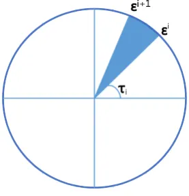
Figure 3. MVN activation function {0, ,τ₁,τk−₁} represents the set of roots of unity by their arguments.

can not only solve multi-valued logic problems but also be differentiable. We call this model “MVN-sig” and its model architecture is illustrated in Figure 5.

Since the activation function is no longer discrete-valued, we need to determine how to obtain the cor- responding label for classification problems. The most intuitive method is to equally divide the mapped range of the activation function. This label judgement method is illustrated in Figure 6.

3.2. Learning Single Neuron Using Gradient Descent Method

Because the MVN-sig a complex-valued neuron, the output of MVN-sig can be derived from input:

, , , ,

= , =

j j re j im j j re j im

x x +x w w +w (8) where x_j,re and x_j,im indicate the real and imaginary parts of _jth

input variable, respectively. Likewise, re

j

w_, and w_j,im indicate the real and imaginary parts of _jth

weight. Thus, the weighted sum of a given n-variable instance can be written as:

, , , , , , , ,

=0 =0 =0

= = ( ) ( )

n n n

j j j re j re j im j im j im j re j re j im

j j j

z

∑

∑

∑

Let the output of MVN-sig be 2

2

2) ( )=

( = =

ˆ_t a_t ib_t cosθ isinθ eiθ

y + + . For an instance t, at and bt are

the real and imaginary parts of MVN-sig output, respectively.

2 2 1 1

ˆ = = ( ) ( ) = ( ( )) ( ( )) = ( ( ( ))) ( ( ( )))

t t t

y a ib cos isin cos F isin F

cos F arg z isin F arg z

θ θ θ θ

+ + +

+ (10)

Figure 5. MVN-sig model architecture.

The error function for an instance t is defined as:

1

ˆ

= , =

2

t t t t t t

E δ δ δ y −y (11)

where yt is the desired output and yˆt is the actual output of MVN-sig neuron. δt is the error between the

desired value and the output. δt signifies the complex conjugate of δt. Let the desired output be yt =αt +iβt.

) ( ) ( = ˆ

= t t t t t t

t y −y α −a +i β −b

δ . Hence, the error function Et is a real scalar function:

} ) ( ) {( 2 1 = 2 1

= t t t t 2 t t 2

t a b

E δδ α − + β − (12)

In order to use the chain rule to find the gradient of error function Et, we have to calculate both real and

imaginary parts independently. In Equation (12), we observe that Et is a function of both (αt−at) and

)

(βt−bt , and at and bt are both functions of wj,re and wj,im. We defined the gradient of the error func- tion Et with respect to the complex-valued weight wj as follows:

, ,

= ( ) = ( )

def

t t t

j

j j re j im

E E E

w i

w w w

η ∂ η ∂ ∂

∆ − − +

∂ ∂ ∂ (13)

The gradient of the error function with respect to the real and imaginary parts of w_j can be written as:

, , , ( ( )) ( ) = ( ) ( ( )) ( ) ( ( )) ( ) ( ) ( ( )) ( )

t t t

j re t j re

t t

t j re

E E a F arg z arg z

w a F arg z arg z w

E b F arg z arg z

b F arg z arg z w

∂ ∂ ∂ ∂ ∂ ∂ ∂ ∂ ∂ ∂ ∂ ∂ ∂ ∂ + ∂ ∂ ∂ ∂ (14) , , , ( ( )) ( ) = ( ) ( ( )) ( ) ( ( )) ( ) ( ) ( ( )) ( )

t t t

j im t j im

t t

t j im

E E a F arg z arg z

w a F arg z arg z w

E b F arg z arg z

b F arg z arg z w

∂ ∂ ∂ ∂ ∂ ∂ ∂ ∂ ∂ ∂ ∂ ∂ ∂ ∂ + ∂ ∂ ∂ ∂ (15)

We can combine Equation (14) and Equation (15) into Equation (13):

, , = { } ( ( )) ( ( )) ( ( )) ( ) ( ) { }{ } ( )

t t t t

j

t t

j re j im

E a E b

w

a F arg z b F arg z

F arg z arg z arg z

i

arg z w w

η ∂ ∂ ∂ ∂

∆ − +

∂ ∂ ∂ ∂

∂ ∂ ₊ ∂

∂ ∂ ∂

(16)

Firstly, we derive each term within the first braces in Equation (16) from Equation (12) and Equation (10):

) ( = ) (

= _{t t t}

t

t _{a Re}

a

E _{α δ}

− − − ∂ ∂ (17) ) ( = ) (

= _{t t t}

t

t _{b Im}

b E

δ

β − −

− ∂ ∂ (18) ))) ( ( ( = )) ( ( ))) ( ( ( = )) (

( F arg z sin F arg z

z arg F cos z arg F a_t − ∂ ∂ ∂ ∂ (19) ))) ( ( ( = )) ( ( ))) ( ( ( = )) (

( F arg z cos F arg z

z arg F sin z arg F b_t ∂ ∂ ∂ ∂ (20)

Equation (16) contains the derivative of the multi-valued sigmoid activation function. We can derive this acti- vation function in Equation (6):

( ( ) )

1 1

( ( ) ) ( ( ) )

=1 =1

( ( )) 2 / 2 exp

= =

( ) ( ) 1 exp 1 exp

c arg z

k k i

c arg z _i c arg z _i

i i

F arg z k c

arg z arg z k

τ

τ τ

π π − −

− −

− − − −

∂ ∂

∂ ∂

∑

∑

Finally, the third braces in Equation (16) contains the derivatives of the argument of weighted sum z. The derivation is shown as follows:

1 2 2 ( ) ( ) ( ) ( ) ( ) ( ) = ( ) = ( ) ( ) ( ) j j

arg z Im z Re z Im z Re z Im z

tan

w w Re z Re z Im z

− ′ ′

∂ ∂ −

∂ ∂ + (22)

where Re(z) and Im(z) represent the real and imaginary parts of weighted sum z and Re′(z) and Im′(z)

represent their derivatives, respectively. From Equation (9), we can simplify this equation:

), ( = ) ( ), ( = ) ( , , j re j j re j x Im w z Im x Re w z Re ∂ ∂ ∂ ∂ (23) ) ( = ) ( ), ( = ) ( , , j im j j im j x Re w z Im x Im w z Re ∂ ∂ − ∂ ∂ (24)

where Re(x_j) and Im(x_j) represent the real and imaginary parts of jth input variable x. Thus, the derivatives of the argument of weighted sum with respect to the real (wj,re) and imaginary wj,im parts is shown as follows:

)) ( ) ( ) ( ) ( ( | | 1 = ) ( 2 , j j re j x Re z Im x Im z Re z w z arg ₋ ∂ ∂ (25) )) ( ) ( ) ( ) ( ( | | 1 = ) ( 2 , j j im j x Im z Im x Re z Re z w z arg ₊ ∂ ∂ (26) j im j re j x z z i w z arg i w z arg 2 , , | | = ) ( ) ( ∂ ∂ + ∂ ∂ (27)

where xj represents the complex conjugate of

th

j input variable x. From Equations (17)-(21) and (27), we can generate the learning rule of jth input weighting ∆wj:

( )

1 1

2 2 (₁ ) 2

=1 2 exp = { ( ) ( ) ( ) ( )}{ }{ } | | 1 exp c k i

j t t c _i j

i

c z

w Re sin Im cos i x

k z

θ τ

θ τ π

η δ θ δ θ − −₋ −₋

∆ − −

+

∑

where θ1 is the argument of the weighted sum and θ2 is the output of multi-valued sigmoid activation func-

tion (F(θ₁)).

3.3. Stopping Criteria

We combine two stopping criteria to make sure the learning process stops when the output is accurate and stable. Firstly, we continue to iterate until the difference between the network response and the target function reaches some acceptable level. In Equation (29), we keep tracking the mean squared error until it reaches a given value

λ. Secondly, we check the relative change in the training error is small using Equation (30). λ

δ

δ ≤

∑

N

t

where N is the total number of learning instances, δt is the error between desired value and estimation, and

) (wt

E and E(wt−1) represent the mean squared errors at tth and (t−1)th learning epochs.

Figure 7 shows two examples of error convergence. Vertical and horizontal axis represent mean squared error and time epoch, respectively. In Figure 7(a), if we only use Equation (30) as the stopping criterion, the learning process will stop early and has worse training and testing accuracy. On the other hand, if we do not use Equation (30), it will take too much time to converge. In Figure 7(b), we can see the learning process is relatively stable after 300 epochs. We monitored the testing accuracy at 300 epoch and at the end of learning process. They did not change much during this interval and that is why we use Equation (29) and Equation (30) as our stopping criteria.

3.4. MVN-Sig Learning Algorithm

We develop the learning algorithm based on the multi-valued sigmoid function and the gradient descent method. The convergence of the learning algorithm can be proven based on the convergence of the gradient descent method in [8]. The implementation of the proposed learning algorithm in one iteration consists of the following steps:

procedure MVN-sig

This is one learning epoch with N learning instances Let i=1 represents the ith instance

Let z be the current value of weighted sum.

s

z

P( )=ε / Equation (10) /

s q ε

ε

δ← −

while i≤N do

Check equation with activation function. for j = 0 to n do / n-variable instance /

j r j r

j w w

w+1← +∆ / Equation (28) / end for

n r n r

r _{w x w x}

w

z 1

1 1 1 1 0 =

~ + ₊ + _++ +

) ~ (z P

q₋ ←ε δ

1 =i+ i end while

Iterates until the outcome meets stopping criteria. / Equation (29) and Equation (30) / end procedure

4. Simulation Results

The proposed strategies and learning algorithms are implemented and checked over a given three benchmark

(a) (b)

datasets [9]. The software simulator is written in Matlab R2011b (64-bit) running on a computer with AMD Phenom II X4 965 3.4 GHz CPU and 8 GB RAM.

4.1. Wine Dataset

This dataset is downloaded from the website of UC Irvine Machine Learning Repository [9]. It contains 178 instances and, for each instance, there are 13 real-valued input variables. The instances belongs to any of the 3 classes that indicates 3 different types of wines.

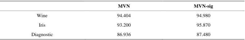
To solve this classification problem, we use 5-fold cross-validation. The first fold has 136 instances in the training set and 42 instances in the testing set. The other 4 folds have 144 instances in the training set and 34 instances in the testing set, respectively. For MVN, we used the testing set to compute their average classi- fication performance after learning with the training set completely with no training error, i.e., training accuracy being 100%. For MVN-sig, we computed their average classification performance after learning process met the stopping criteria. The testing accuracy obtained by MVN and MVN-sig, respectively, for this dataset, is shown in Table 1. From this table, we can see that MVN-sig achieves a better testing accuracy than MVN.

4.2. Iris Dataset

This well known dataset is also downloaded from the website of UC Irvine Machine Learning Repository [9]. It contains 150 instances and, for each instance, there are 4 real-valued input variables. The instances are belong- ing to any of the 3 classes (Setosa: 0, Versicolour: 1 and Virginica: 2).

To solve this classification problem, we use 5-fold cross-validation. The dataset is randomly divided into 120 instances of training set and 30 instances of testing set. For MVN, the learning process will not stop after 10,000 iterations if we want to learn whole instances with no error, i.e., training accuracy being 100%. The training accuracy of our MVN-sig algorithm is from 96% to 99%, and we choose 96% to be the stopping criterion for MVN learning. For MVN-sig,we computed their average classification performance after learning process met the stopping criteria. The testing accuracy obtained by MVN and MVN-sig, respectively, for this dataset, is shown in Table 1. From this table, we can see that MVN-sig achieves a better testing accuracy than MVN.

4.3. Breast Cancer Wisconsin (Diagnostic) Dataset

This is also downloaded from the website of UC Irvine Machine Learning Repository [9]. It contains 569 instances and, for each instance, there are 32 real-valued input variables. The instances are belonging to 2 classes (malignant: 0 and benign: 1).

To solve this classification problem, we use 5-fold cross-validation. The first fold has 452 instances in the training set and 117 instances in the testing set. The other 4 folds have 456 instances in the training set and 113 instances in the testing set, respectively. For MVN, we used continuous learning rule in Equation (5) since the discrete one is not suitable for binary classification. We used the testing set to compute their average classification performance after learning with the training set completely with no training error, i.e., training accuracy being 100%,. For MVN-sig,we computed their average classification performance after learning process met the stop- ping criteria. The testing accuracy obtained by MVN and MVN-sig, respectively, for this dataset, is shown in Table 1. From this table, we can see that MVN-sig achieves a better testing accuracy than MVN.

5. Conclusions and Discussions

The parameter c in Equation (6) affects the converging time and performance. We can develop a parameterfree model since the activation function of MVN-sig is differentiable. But if we make this model parameter-free, the

Table 1. Accuracy comparison of MVN and MVN-sig.

MVN MVN-sig

Wine 94.404 94.980

Iris 93.200 95.870

execution time is increased tremendously. In this paper, we select suitable parameters for each experiment. The simulation results obtained with benchmark datasets show MVN-sig meets our expectation of original thoughts. From the result of Iris dataset, we can see if we loosen the MVN stopping criterion, MVN-sig can still achieve better testing accuracy. But the critical downside is the much higher time complexity. In this paper, we just apply a simple gradient descent method to the neuron. More complicated techniques for reducing back- propagation time can be applied.

There are three main concerns about the future work of the MVN-sig neuron. Firstly, we have to develop a multilayer neural network using MVN-sig and investigate its performance. Secondly, to reduce its execution time we need to do more research on the learning algorithm. Finally, we have to find its pros and cons in the real-world applications.

References

[1] Aizenberg, N.N. and Aizenberg, I.N. (1992) CNN Based on Multivalued Neuron as a Model of Associative Memory For Grey Scale Images. In Proceedings of Second IEEE International Workshop on Cellular Neural Networks and their Applications (CNNA-92), 36-41. http://ieeexplore.ieee.org/stamp/stamp.jsp?arnumber=274330

[2] Aizenberg, I., Aizenberg, N.N. and Vandewalle, J.P. (2000) Multi-Valued and Universal Binary Neurons: Theory, Learning and Applications. Springer. http://dx.doi.org/10.1007/978-1-4757-3115-6

[3] Aizenberg, I. and Moraga, C. (2007) Multilayer Feed Forward Neural Network Based on Multi-Valued Neurons (mlmvn) and a Backpropagation Learning Algorithm. Soft Computing—A Fusion of Foundations, Methodologies and Applications, 11, 169-183. http://www.springerlink.com/index/T645547TN41006G0.pdf

[4] Aizenberg, I., Paliy, D.V., Zurada, J.M. and Astola, J. T. (2008) Blur Identification by Multilayer Neural Network Based on Multivalued Neurons. 19, 883-898. http://ieeexplore.ieee.org/stamp/stamp.jsp?arnumber=4479859

[5] Aizenberg, I. (2010) Periodic Activation Function and a Modified Learning Algorithm for the Multivalued Neuron. 21, 1939-1949. http://ieeexplore.ieee.org/stamp/stamp.jsp?arnumber=5613940

[6] Aizenberg, I. (2011) Complex-Valued Neural Networks with Multi-Valued Neurons. Springer.

[7] Wilson, E. (1994) Backpropagation Learning for Systems with Discrete-Valued Functions. Proceedings of the World Congress on Neural Networks, San Diego, California, June.

[8] Hagan, M.T., Demuth, H.B., Beale, M.H., et al. (1996) Neural Network Design. Thomson Learning Stamford, CT.