D irect S im u lation M eth o d s
for M u ltip le C h an gep oin t
P rob lem s
Zhen Liu, B .S c.
Subm itted for the degree of Doctor of Philosophy
at Lancaster University,
ProQuest Number: 11003426
All rights reserved
INFORMATION TO ALL USERS
The qu ality of this repro d u ctio n is d e p e n d e n t upon the q u ality of the copy subm itted.
In the unlikely e v e n t that the a u th o r did not send a c o m p le te m anuscript and there are missing pages, these will be note d . Also, if m aterial had to be rem oved,
a n o te will in d ica te the deletion.
uest
ProQuest 11003426
Published by ProQuest LLC(2018). C op yrig ht of the Dissertation is held by the Author.
All rights reserved.
This work is protected against unauthorized copying under Title 17, United States C o d e M icroform Edition © ProQuest LLC.
ProQuest LLC.
789 East Eisenhower Parkway P.O. Box 1346
2
D irect S im u lation M eth o d s for
C h an gep oin ts P ro b lem s
Z hen Liu B .S c
D epartm ent of M athem atics and S tatistics
Fylde College, Lancaster University
Subm itted for the degree of D octor of Philosophy
at Lancaster University, Septem ber 2007.
A b str a c t
The multiple changepoint model has been considered in a wide range of statistical
modelling, as it increases the flexibility to simple statistical applications. The main
purpose of the thesis enables the Bayesian inference from such models by using the
idea of particle filters. Compared to the existed methodology such as RJM CMC
of Green (1995), the attraction of our particle filter is its simplicity and efficiency.
We propose an on-line algorithm for exact filtering for a class of multiple change
point problems. This class of models satisfy an im portant conditional indepen
dence property. This algorithm enables simulation from the true joint posterior
distribution of the number and position of the changepoints for a class of change
point models. The com putational cost of this exact algorithm is quadratic in
the number of observations. We further show how resampling ideas from particle
filters can be used to reduce the com putational cost to linear in the number of
observations, at the expense of introducing small errors; and propose two new,
optim um resampling algorithms for this problem. In practice, large com putational
savings can be obtained whilst introducing negligible error. We dem onstrate how
th e resulting particle filter is practicable for segmentation of human GC content.
3
property does not hold. In particular we consider models w ith dependence of the
param eters across neighbouring segments.
Examples of such models are those w ith unknown hyper-param eters, and piecewise
polynomial regression models which assume continuity of the regression function.
The particle filter we propose is based on a simple approxim ation to the filtering
recursion. We show th a t the error introduced by the approxim ation can be small.
We dem onstrate our m ethod on the problem o f Bayesian curve fitting. The novelty
of our model is th a t we fit a piecewise polynomial function and allow for both
discontinuity and continuity a t changepoints. This m ethod is compared to existing
D ecla ra tio n
I declare th a t th e work presented in this thesis is my own, except where stated
otherwise. The work of C hapter 4 is based on the publication of Fearnhead and
Liu (2007).
The algorithms developed in C hapter 4 and 5 are coded by myself in a combi
nation of R and C + + programming languages. The tem plate numerical toolkit
(TNT) developed by N ational Institute of Science and Technology (NIST) is used
for m atrices m anipulation.
Zhen Liu
A ck n ow led g m en ts
I am very grateful to my supervisor, Professor Paul Fearnhead. I feel very lucky
to be supervised by him in the past three years. His innovative thoughts, modest
attitu d e and remarkable achievement in his research work has been inspired me
throughout my PhD study. He has been extremely supportive of me, as he has
shown great patience to check every line of my code and thesis. He also provided
me a lot of chances to atten d different training and conferences.
I am also very grateful to Dr Joe W hittaker, for his encouragement and guidance
in th e first year of my PhD study. W hen I arrived this country th a t is more th an
10,000 miles away from home for the first tim e,it was him who made me confident
to finish this thesis.
My life at Lancaster would have been different without a friendly environment.
In particular, I would like to thank Dongfang Shi, David Yen, Hongsheng Dai,
Yanchun Bao, Peter Henrys, Tristan Marshall, Ting-li Su and Vilda Purutcuoglu
for their friendship, advice and invaluable discussions. I would also like to thank
the football team m ates in the departm ent. The game with them made me very
energetic in the academic research.
Of course, I would like to thank my parents for their supports in all aspects. They
spent countless time and energy to make me a doctor without thinking of any
reward. However, it is time to reward them now. Two friends from the other side
of the A tlantic Ocean are worth mentioning: Dan Liao and Junling Xiong. I would
6
like to take the chance to than k they two.
Finally, I gratefully acknowledge the financial support for this project given by the
C o n ten ts
1 I n tr o d u c ti o n 1
1.1 R e tro s p e c t... 1
1.1.1 Rejection s a m p lin g ... 2
1.1.2 Markov chain Monte C a r lo ... 3
1.2 M o tiv a tio n ... 4
1.2.1 Im portance s a m p lin g ... 5
1.2.2 Sequential Monte Carlo m e t h o d ... 6
1.3 Outline of the thesis ... 8
2 P a r t i c le filte rs 10 2.1 In tro d u c tio n ... 10
2.1.1 The basis of particle f il te r s ... 11
2.1.2 Resampling in particle filte rs ... 13
2.1.3 Sampling importance resampling ... 14
C O N T E N T S ii
2.1.4 W hen to resam p le... 16
2.2 Sampling a lg o r ith m s ... 17
2.2.1 Sequential im portance s a m p lin g ... 18
2.2.2 Auxiliary SIR f i l t e r ... 20
2.2.3 O ther sampling a lg o rith m s ... 23
2.3 Resampling a lg o rith m s ... 24
2.3.1 Stratified s a m p l in g ... 24
2.3.2 Rejection control ... 26
2.3.3 Optim al re sam p lin g ... 28
2.3.4 MCMC m o v e ... 31
2.4 Smoothing p ro c e d u re ... 33
2.4.1 Smoothing by storing particle h i s t o r y ... 33
2.4.2 Forward-backward s m o o th in g ... 36
2.4.3 Two-filter s m o o th in g ... 37
3 C h a n g e p o in ts m o d e ls 40 3.1 In tro d u c tio n ... 40
3.2 D istribution of changepoints ... 42
C O N T E N T S iii
3.4 Particle filter a p p r o a c h ... 47
3.4.1 M ixture Kalman f i l t e r ... 48
3.4.2 Rao-Blackwellised particle f i l t e r ... 51
4 O n -lin e in fe re n c e fo r m u ltip le c h a n g e p o in t p ro b le m s 57 4.1 In tro d u c tio n ... 57
4.2 Models and N otations ... 59
4.3 On-line I n f e r e n c e ... 62
4.3.1 Exact on-line In fe re n c e ... 63
4.3.2 Approximate In f e re n c e ... 66
4.4 Numerical E x a m p le s ... 73
4.5 DNA S e g m e n ta tio n ... 79
4.6 Discussions ... 81
4.7 A p p e n d i x ... 85
5 E ffic ien t B a y e s ia n A n a ly sis o f M u ltip le C h a n g e p o in t M o d e ls w ith D e p e n d e n c e a c ro ss S e g m e n ts 91 5.1 In tro d u c tio n ... 91
5.2 Changepoint model ... 94
C O N T E N T S iv
5.3.1 Filtering recursion ... 102
5.3.2 Filtering with resam p lin g ...107
5.4 Backward s m o o th in g ... 108
5.5 Param eter e s tim a tio n ...112
5.6 Evaluation of m e th o d o lo g y ... 112
5.6.1 Accuracy ...113
5.6.2 Im portance w e ig h ts ... 119
5.7 Simulation studies ... 122
5.7.1 Smooth curves ...124
5.7.2 Unsmooth c u r v e s ...126
5.7.3 Further co m p ariso n ... 134
5.8 Well-log d a t a ...135
5.8.1 Historical m e th o d o lo g ie s...136
5.8.2 Model and p r i o r ...136
5.8.3 R e s u lts ... 138
5.9 Discussions ... 138
5.10 A p p e n d i x ... 141
L ist o f F igu res
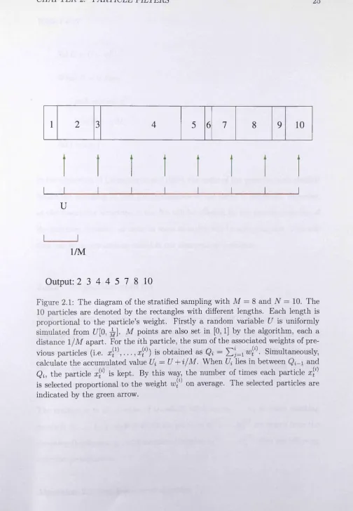
2.1 The diagram of the stratified sampling w ith M = 8 and N = 10.
The 10 particles are denoted by the rectangles w ith different lengths.
Each length is proportional to the particle’s weight. Firstly a ran
dom variable U is uniformly simulated from U[0, ^ ] . M points
are also set in [0,1] by the algorithm, each a distance 1 /M apart.
For the ith particle, the sum of the associated weights of previous
particles (i.e. x ^ \ . . . , x ^ ) is obtained as Qi = Yl)=i wt^ ■ Simulta
neously, calculate the accumulated value Ui = U + i / M . W hen Ui
lies in between Qi_i and Q i, the particle is kept. By this way,
the number of times each particle is selected proportional to the
weight w® on average. The selected particles are indicated by the
L IS T OF FIG U R ES
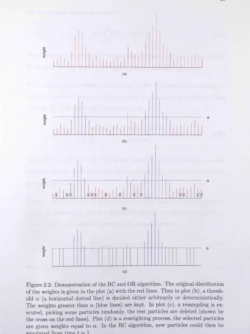
2.2 D em onstration of the RC and OR algorithm. The original distri
bution of the weights is given in the plot (a) with the red lines.
T hen in plot (b), a threshold a (a horizontal dotted line) is decided
either arbitrarily or deterministically. The weights greater th an a
(blue lines) are kept. In plot (c), a resampling is executed, picking
some particles randomly, the rest particles are deleted (shown by
the cross on the red lines). Plot (d) is a reweighting process, the
selected particles are given weights equal to a. In the RC algorithm,
new particles could then be simulated from tim e t = 1...
2.3 A diagram of particle filters running from tim e 1 to 7. There are
10 dots at each time, which represent 10 particles with different
weights. Each particle will give birth to new particles at next time.
Only the particles selected by resampling algorithm will survive and
are presented at each time. The arrows indicate the relationship
between the particle and its off-springs. The same color means the
particles have a common ancestor. The history of each particle can
be seen very clearly in this way, and we can find th a t how quickly
th e number of distinct ancestors of particles reduces as we go back
over time. For example at time 7, it is obvious th a t all the particles
are generated by two distinct particles at tim e 1...
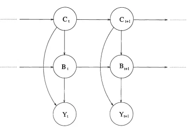
3.1 A state space model for changepoints problem. The underlying state
consists of two components: the changepoint Ct and the param eter
B t . Ct stands at the top hierarchy of the model and takes some
discrete values in a finite space. So it can be seen as an indicator
function. In contrast, B t and Yt is modelled can take a value in a
continuous space. Conditional on Ct , a relationship between B t and
L IS T OF FIG U R ES vii
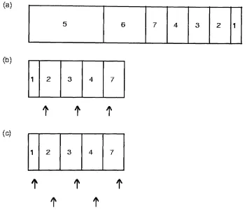
4.1 Example of the stratified resampling algorithm as used in SOR or
SRC. (a) Example set of particles. Each box represents a particle,
labelled with its value (the time of the most recent changepoint),
and whose w idth is proportional to its weight. Particle 5 has weight
0.3; particle 6 has weight 0.25; particles 2-4 and 7 each have weight
0.1; and particle 1 has weight 0.05. (b) Stratified resampling within
SOR to resample 5 particles. In this case a — 0.15 and p arti
cles 5 and 6 are kept w ithout resampling. The remaining particles
are ordered as shown, with 3 to be resampled. A uniform random
variable, [/, on [0, a] is simulated, and 3 arrows are produced at
positions U, U + a, and U + 2a. The particles which are pointed
to by the arrows are resampled and are each assigned a weight a.
(c) Stratified resampling within SOR with a — 0.2. Again particles
5 and 6 are kept w ithout resampling, and the remaining particles
are ordered. We again simulate [/, a uniform random variable on
[0, a], and place arrows at U, U + a, U + 2a an so on. In this case
the number of arrows needed, and hence the number of particles
resampled, will depend on U. We show two possible set of arrows
for this example, the top set produces 3 resampled particles, and
the bottom set 2. Each resampled particle is assigned a weight a. . 69
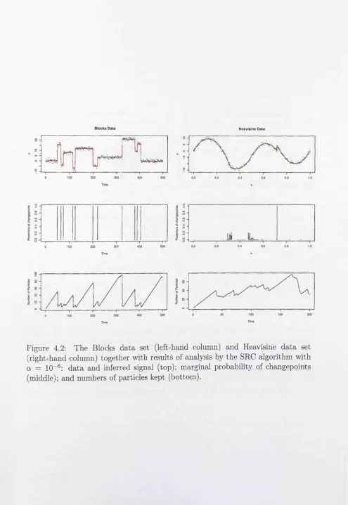
4.2 The Blocks d a ta set (left-hand column) and Heavisine d a ta set
(right-hand column) together with results of analysis by the SRC
algorithm w ith a = 10-6 : d ata and inferred signal (top); marginal
probability of changepoints (middle); and numbers of particles kept
L IS T OF FIG U RES viii
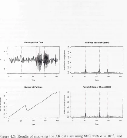
4.3 Results of analysing the AR d a ta set using SRC with a — 10-6 ,
and the particle filter of Chopin (2007) with 50,000 particles: d ata
(top left), marginal probabilities of changepoint for SRC (top right)
and particle filter of Chopin (2007) (bottom right), and number
of particles kept using SRC (bottom left). The true AR model
to th e four segments have model orders 1, 1, 2, and 3 respec
tively. The corresponding param eters are [Ik = 0.4; [3k = —0.6;
(3k = (—1 .3 ,-0 .3 6 ,0 .2 5) and (3k = (—1 .1 ,—0.24) w ith error vari
ances 1.22, 0.72, 1.32 and 0.92 respectively... 76
4.4 Analysis of 3.6 Mb of d ata from the MHC region. The d ata consist
of number of C + G nucleotides in 3kb windows. We show 20 reali
sations from the joint posterior distribution of the segmentation. . 82
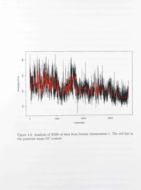
4.5 Analysis of 35Mb of d ata from human chromosome 1. The red line
is th e posterior mean GC content... 83
5.1 An example of a dependent changepoint and an independent change
point. The vertical dotted line indicates the position of changepoint. 97
5.2 An example of a continuous changepoint and a discontinuous change
point. The vertical dotted line indicates the position of changepoint 97
5.3 A dem onstration of Ct , M t and 0 t and their values (shown in the
L IS T OF FIG U R ES
5.4 The plots on the left show the two different marginal posterior dis
trib u tio n of the position of change point,i.e. p (C \y i:n) (The ap
proxim ated distribution is actually p{Cn\Cs = 0 ,y i:n)). The plots
on the right show the two different joint posterior distribution, i.e.
p ( C , M|y 1:n). (Red line: Approximated distribution; Blue line: Ex
act d is trib u tio n )...
5.5 Left panels: The three lines in each plot are true curve (green solid
line), fitted curves by approxim ated algorithm (red dash line) and
by exact algorithm (blue dash line), respectively. All the curves are
produced by averaging across 100 independent realisations. Right
panels: The three lines in each plot are differences between every
two curves over time. The red line is th a t between approximately
fitted and true curves. The blue line is th a t between exactly fitted
and true curves. The green line is th a t between approximately fitted
and exactly fitted curves...
5.6 The im portance weights from 1000 replicates of simulations and
the fitted curves, each of which is an average of 1000 realisations,
chosen from the simulation results by the im portance weights we
calculated. Upper: The importance weights and fitted curve of the
Heavisine data. Bottom: The importance weights and fitted curve
of the Blocks d a t a ...
5.7 The im portance weights from 1000 replicates of simulations and
the fitted curves, each of which is an average of 1000 realisations,
chosen from the simulation results by the im portance weights we
calculated. Upper right: The importance weights and fitted curve
of the Bumps data. Bottom: The im portance weights and fitted
L IS T OF FIG U R ES x
5.8 Left plots: The marginal posterior distribution of positions and
types of changepoints p (C t,M t
|yi:*),
red lines represent the dis continuous changepoints and green lines represent the continuouschangepoints. Right plots: The true curves (blue lines) and the
fitted curves (red lin e s ) ... 125
5.9 Heavisine curve. Upper: The marginal posterior distribution of
positions and types of changepoints, p(Ct , M t
|yi:n).
Red lines rep resent the discontinuous changepoints while green lines representcontinuous ones. Middle: the simulated d a ta and the fitted curve.
Bottom: the true curve...127
5.10 The variance of noise, a 2 (red line), and its 95% confidence interval
(blue lines) over tim e...127
5.11 Blocks curve: Upper: The marginal posterior distribution of posi
tions and types of changepoints, p(Ct, M t
|y1:n).
Red lines represent the discontinuous changepoints while green lines represent continuous ones. Middle: the simulated d ata and the fitted curve. The
bottom plot is the true curve... 128
5.12 The variance of noise, a 2 (red line), and its 95% confidence interval
(blue lines) over tim e... 128
5.13 Bumps curve: Upper: The marginal posterior distribution of posi
tions and types of changepoints, p(Ct, M t \y 1:n). Red lines represent
the discontinuous changepoints while green lines represent continu
ous ones. Middle: the simulated d ata and the fitted curve. Bottom:
the tru e curve... 129
5.14 The variance of noise, a 2 (red line) , and its 95% confidence interval
L IS T OF FIG U R ES xi
5.15 Doppler curve: Upper: The marginal posterior distribution of posi
tions and types of changepoints, p(Ct, M t \yi:n). Red lines represent
the discontinuous changepoints while green lines represent continu
ous ones. Middle: the simulated d a ta and the fitted curve. Bottom:
th e tru e curve...130
5.16 The variance of noise, a 2 (red line), and its 95% confidence interval
(blue lines) over tim e...130
5.17 We have compared 4 methodologies on the Heavisine d a ta set. Top
left: the methodology of Denison et al. (1998); Top right: methodol
ogy of DiM atteo et al. (2001); Bottom left: Methodology of Chapter
4; B ottom right: Methodology of our algorithm. The blue dash line
is the true curve and the red line is the fitted curve. The circles in
the bottom plots indicate the slight difference of those two curves. 133
5.18 Plot of well-log d a ta ... 135
5.19 Upper plot: The marginal smoothing distribution of positions and
types of changepoints p{Ct , M t \yhn). Green lines indicate the con
tinuous changepoints and blue lines indicate discontinuous change
points. B ottom plot: The underlying line for well log data. The
d a ta is properly scaled and a piecewise quadratic model is used. . . 139
L ist o f T ables
4.1 Mean Kolmogorov Smirnov Distance in P(Ct \yi-.t) averaged over t
for the Heavisine and AR models and the four resampling algo
rithm s. Stratified Rejection Control (SRC) and Rejection Control
(RC) were implemented with a = 10-6 ; these algorithms used an
average number of 43 and 70 particles for the Heavisine and AR
models respectively. Optimal Resampling (OR) was implemented
w ith N = M + 1 = 49 and N = M + 1 = 90; Stratified Optimal
Resampling (SOR) used N = M + 5 - 51 and TV = M + 5 = 92
(chosen so th a t the average number of particles is the same for all al
gorithms for each d ata set). Results based on 50 replications of each
algorithm for one version of each d ata set. The true distribution,
P(Ct\yi:t), was calculated using the exact on-line algorithm. . . . 5.1 The Root Mean Square Error between every two lines out of the
tru e line, the line produced by approximate algorithm and the line
produced by exact algorithm. D ata Set 1, 2 and 3 correspond to
the top left, top right and bottom left plots of Figure 5 . 5 ...
5.2 The effective sample size (ESS) of each d ata set based on the 1000
L IS T OF T A B L E S xiii
5.3 Mean square error of each methodology on the sm ooth curves in
Figure 5.8. The MSE of D PF is calculated based on (a)z/ = 6250,
7 = 1000 (so th a t F ( a 2) = 0.42); and (b) v = 11111,7 — 1000 (so
th a t E(<j2) = 0.32) 126
5.4 Mean square error of each methodology on the unsm ooth functions
in Figure 5.9-5.15. The MSE of D PF is calculated base on v = 1000
C h ap ter 1
In tro d u ctio n
1.1
R e tr o sp e c t
Sampling-based Bayesian statistical methods have been very popular in the last 20
years because of its simplicity in approximating the intractable integrals involved
w ith the inferential problem, particularly in high dimensions. All these methods
are based on the Monte Carlo integration, in which a set of samples x^ , . . . , x ^
are independently simulated from a target distribution of random variable X with
probability density function p(x). Then we can use these samples to approximate
the expectation of any function h(-) of X , provided the expectation exists. T h at
is if we want to calculate
( i . i )
we can approximate it by a sample mean
(1.2)
C H A P T E R 1. IN TR O D U C TIO N 2
The approach is remarkably easy to use and gives an unbiased estim ate with
variance proportional to 1 /N (i.e. vax(h(x))/N ) .
In particular, if we take h(x) — Ia{x) where Ia(x) is an indicator function so th a t
it takes value 1 if x £ A and value 0 otherwise, then the probability Pr(a; E A) are
approxim ated only by the proportion of samples in A:
P r(x
e
A) = E (JA(x)) » ^ £U (*w).
t= l1.1.1
R e je c tio n sa m p lin g
However, It is often the case th a t we are unable to simulate directly from the
target density p(-). A sensible m ethod to overcome the problem is to simulate
from another density q(-) which is easy to simulate from, but then to only accept
those samples w ith a probability paccept- This is the basic idea of rejection sampling
(Hammersley and Handscomb, 1964).
To run the method, we only need to know the target density p(-) up to a normal
ising constant, and have to set an upper bound K such th a t
p (x )/q (x) < K for all x,
therefore the support of q(-) contains all the support ofp(-). The sampling proce
dure is done as follows:
A lg o r ith m 1.1 Rejection sampling
S te p 1 Simulate x from the proposal density q(x);
C H A P T E R 1. IN T R O D U C T IO N 3
S te p 3 Generate a random variable U uniformly from the interval [0,1];
S te p 4 I f U < paccept accept x; otherwise repeat.
Then xs accepted by this algorithm are independent identically distributed (i.i.d)
samples from the target distribution. Furthermore, the average acceptance prob
ability is 1 /K .
The efficiency of the rejection sampling is dependent on the upper bound K , and
particularly the dimensions of the target distribution. The acceptance probability
decreases exponentially as the dimension increases.
1.1.2
M arkov ch ain M o n te C arlo
If we run the rejection sampling iteratively over an irreducible and aperiodic
Markov chain whose equilibrium distribution is the target distribution, this is
the intuitive idea behind Markov chain Monte Carlo (MCMC).
The main difficulty of MCMC is how to construct a suitable Markov chain to
enable a simulation from the target distribution. A general algorithm which they
call Metropolis-Hasting algorithm is proposed by Metropolis et al. (1953) and then
generalised by Hasting (1970). The algorithm requires a transition kernel k (x ,x ')
for the Markov chain, which is a proposal density function of x' for each given
value of x. Thus at each iteration, a sample x' is drawn from the kernel k (x ,x '),
and the new value x in the chain is
x = <
x' with probability paccept,
(1.3)
C H A P T E R 1. IN T R O D U C TIO N 4
where
. f k(x', x)p(x') 1 .
P a c c e p t = mm S 1 , 7 /W \ f ' ( l - ^ )
t k(x, x')p(x) J
The initial value of x can be chosen arbitrarily. Then Tierney (1994) has proved
th a t the Markov chain obtained by the above algorithm is time-reversible and has
an equilibrium distribution p(-).
The transition kernel can be chosen arbitrarily as well, in principle, so any choice
should work. However, not all kernels are equally good w ith respect to the con
vergence property (or mixing property) of the algorithm. Common choices include
fully conditional distribution (in Gibbs sampling) and random walk with normal in
crement (in random walk Metropolis algorithm). For a complete review of MCMC,
see Gilks et al. (1996); Robert and Casella (1999). Note th a t MCMC does not
provide independent draws from p(-); but Monte Carlo estim ators such as (1.2)
will still be consistent.
1.2
M o tiv a tio n
The MCMC m ethod has been very successful since the beginning of 1990s, because
of its flexibility to a lot of statistical models. It is a popular approach to sample
different complicated probability distributions. However, there are still some limi
tations of MCMC m ethod in some situations. For example, it is inefficient for the
recursive estim ation problems. Hence, we introduce in the thesis another sampling
C H A P T E R 1. IN T R O D U C T IO N
1 .2.1
Im p o r ta n c e sa m p lin g
5
There might be another problems with d(p) as an estim ator of d: although sam
pling from p(-) is possible, the estim ator $(p) might have very high variance.
Instead, an importance sampling technique (see Geweke, 1989, for example) can be
used to overcome the problem. We can choose another distribution of the random
variable X w ith density q(x), from which, the samples a^1), . . . , x ^ can be easily
simulated. Thus, we can rewrite D as
$ = [ h(x)^Y^-q(x)(Ix, (1.5)
J q{x)
and it can be approxim ated by
N
$(q) = (1.6)
i= 1
where we define th e (normalised) importance weight as
w<<)« ErS'
f > w = 1-
(L7)
Thus the im portance sampling is basically choosing the samples concentrated on
th e area where there is greatest variation in the integrand so th a t each simulated
value contains greatest information. If we choose q(-) so as to make h{x)p(x)/q{x)
nearly constant, the variance of ti(q) will be much lower th an the variance of $(p).
C H A P T E R 1. IN T R O D U C T IO N
where the im portance weight w® is
6
«»<*> = (1 9)
q(x®) 1 J
instead. However, in many applications, the target probability p(-) and the pro
posal density q(-) may be known only up to a normalising constant. This is always
tru e when applying the im portance sampling to the state space model and, par
ticularly in Bayesian statistics. Hence the use of normalised im portance weights
is more general.
1.2.2
S eq u e n tia l M o n te C arlo m e th o d
Im portance sampling has a wider scope th an reducing the variance of Monte Carlo
estimators. This thesis will concentrate on the im portance sampling in the sequen
tial settings, which is also known as particle filters (Doucet et al., 2001; Liu, 2001).
The technique has been commonly used in time series model for some dynamic
problems such as target tracking (Gordon et al., 1993), signal deconvolution (Liu
and Chen, 1995), speech recognition (Godsill and Clapp, 2001), oil drilling (Fearn-
head and Clifford, 2003) and stock pricing (Kitagawa, 1996), amongst others. In
such cases, the new observation becomes available at each time, thus a real time
inference or prediction is required. In other words, a sequence of distributions
7rt , which is the posterior of the underlying states given the observations in the
dynamic system, needs to be estim ated at each time t. A typical example of irt is
th e position and speed of a target at time t in the target tracking problem.
The reason why the importance sampling can be used efficiently to estim ate these
posteriors is th a t the approximate samples from the distribution nt can be recycled
by importance sampling to produce approximate samples from the distribution
C H A P T E R 1. IN T R O D U C TIO N 7
are different, we can augment the supports of 7rt to the supports of 7rt+i, and
simulate the im puted samples to approxim ate 7rt+i (Kong et al., 1994). The biggest
advantage of this sequential computing is th a t the im portance weights at each time
t do not need to be re-computed from the scratch. The dynamic updating produces
a reduction on the com putational cost.
The motivation of the thesis is to consider and develop particle filters for analysis
of multiple changepoint problems. W ith particle filters, we aim to draw samples
directly from the posterior distribution of changepoints.
The multiple changepoints model we use here consists of a sequence of change
points occurring at discrete positions. Both the number and positions of them
are unknown. The MCMC method has been dominant in the Bayesian analysis
of the changepoints models. If the number of changepoints is known, the m ethod
can be directly used for inference in the models (e.g. Stephens, 1994; Chib, 1996).
If the number of changepoints is unknown, a common approach is the reversible
jum p Markov chain Monte Carlo (RJMCMC) method of Green (1995). However,
RJM CM C can suffer from poor mixing, and hence a high CPU cost, unless effi
cient MCMC move can be designed. But this is generally very hard, particularly
for the move between different models in RJM CMC (see Brooks et al., 2003, for
guidelines on how to design these moves).
By contrast, the particle filtering approach to changepoints model is less obvious.
An artificial time has to be given so th a t a pseudo sequence of the posterior
distributions of changepoints can be fed into the particle filters as it were the
targ et distributions arising in a dynamic problem. The particle filtering approach
avoids the diagnosis of the convergence of Markov chains and hence the design of
moves in the MCMC. It is also believed th a t the particle filter approach provides
b etter estimates in term s of robustness and effectiveness.
C H A P T E R 1. IN T R O D U C T IO N 8
the two are not th a t separated. Instead, we can even embed one algorithm into
the other, to improve the performance of the algorithm.
1.3
O u tlin e o f th e th esis
The them e of this thesis is the construction of a direct simulation methodology
based on the particle filters, and the application to the multiple changepoint prob
lems. The m ethod is proposed to enable inference for the changepoint model to
be made more efficiently. The outline of the subsequent chapters is as follows:
In C hapter 2, the basic structure of particle filter including sampling, resampling
and smoothing is introduced. A very simple example which is known as the SIR
filter or B ootstrap filter (Gordon et al., 1993) is given immediately to dem onstrate
how the particle filter works on the non-linear/non-G aussian state space model.
M otivated from the demonstrative example, a number of literature focusing on
improving the performance of the particle filters are reviewed. The improvements
cover all aspects of the particle filters (e.g. sampling, resampling and smoothing).
In C hapter 3, we describe the multiple changepoint problem through a state space
model so th a t the on-line inference can be made. We adapt a point process of Barry
and H artigan (1993) to model the distribution of the positions of changepoints and
th e number of changepoints is autom atically implied. The underlying states have
a hierarchy w ith the changepoints and the associated param eters, which will make
the particle filters introduced in Chapter 2 less accurate and efficient. So it is
advantageous to marginalise the param eter state sequence as nuisance param eters
and focus on the on-line inference of changepoints first. Two specific examples
given by Chen and Liu (2000) and Chopin (2007) respectively are reviewed. The
approach of Chen and Liu (2000) is a special case of Rao-Blackwellised particle
change-C H A P T E R 1. IN T R O D U change-C T IO N
points.
9
The innovative p art of the thesis is C hapter 4. We propose an on-line algorithm
for exact filtering of the multiple changepoint problems. This algorithm enables
simulation from the true joint posterior distribution of the number and position of
th e changepoints for a class of changepoint models. The algorithm is constructed
w ith in a particle filter framework, and we dem onstrate how the resulting particle
filter is practicable for segmentation of human GC content.
In C hapter 5, we extend the multiple changepoint model to allow for dependen
cies across segments and apply it to the curve fitting examples. We propose an
algorithm for approxim ated filtering of the multiple changepoints model and a
smoothing algorithm to detect both the positions and types of changepoints. We
dem onstrate the performance of our algorithm on both smooth and unsmooth
curves, and compare the it with some MCMC method. Practically, we use the
algorithm to analyse well log d a ta from the oil industry. The results are presented
there as well.
In the final chapter, we present some conclusions and point out some further
C h ap ter 2
P a rticle filters
2.1
In tro d u ctio n
Particle filters are sequential Monte Carlo methods based upon point mass (or
“particle” ) representation of probability densities, which are widely applied for
on-line inference of state space models:
X, = f {Xt. u Wt)
Yt = g ( X t,Vt).
Here W t and Vt are sequences of mutually independent random variables of known
distribution. To enable the inferences of the underlying states X t to be made, the
measurements Yt are taken at each discrete time t — 1 , 2 , . . . , n. The underlying
states X t follow a Markov process. We denote the transition probabilities implied
by (2.1) as p (x t+i\xt); and assume a prior distribution for the state at time 1,
p(x i).
If (2.1) are linear equations, and W t and Vt have Gaussian distributions, the
Kalman filter (Kalman and Bucy, 1961) can be used to calculate the posterior
C H A P T E R 2. P A R T IC LE F ILTE R S 11
distribution of the states. If the assumptions fail to hold, some other sub-optimal
algorithm needs to be used, like the particle filter.
The particle filter gives a Monte Carlo approxim ation to the distributions of inter
est. A set of comprehensive reviews of particle filters can be found in Liu and Chen
(1998); Doucet et al. (2001); Arulampalam et al. (2002). The use of Monte Carlo
m ethods in filtering can be traced back to the pioneering contribution of Hand-
schin and Mayne (1969) and Handschin and Mayne (1970), in which the Monte
Carlo methods are used only to estim ate the mean and covariance of the posterior.
A nother earlier sequential Monte Carlo methods was proposed by West (1992)
when filtering w ith the mixture probability densities. Alternatives to the particle
filters include the extended Kalman Filter (Jazwinski, 1973; Anderson and Moore,
1979), the Gaussian sum filter (Sorenson and Alspach, 1971) and the approximate
grid-based m ethods (Bucy and Senne, 1971). See also West and Harrison (1997)
for a complete review.
2 .1 .1
T h e b asis o f p a rticle filters
The aim of the particle filter is to estim ate recursively in tim e the posterior distri
bution of states p (x i:t|yi;t) (where x i:* := ( z i , . . . , x t) and y i ;t := {yx, . . . , yt)), or
the m arginal distribution p (x t \yi:t) (also known as the filtering distribution), and
consequently, some functions of the states, e.g. the expectations E p(h (X t)). We
focus on the filtering distribution in this thesis.
At any tim e t, the marginal distribution p (x t|ym) is given by B a yes’ theorem
Although the recursions of posterior p (x t \y1:t) are easily obtained, solving them
(2.2)
p (x t \yi:t)
J
p(yt \xt)p(xt \y1:t - l ) d x t ' p(yt\xt)p(xt\yi:t-i)C H A P T E R 2. P A R T IC LE F ILTE R S 12
is normally intractable, as it involves the evaluation of complex high-dimensional
integrals in calculating f p{yt\xt)p{xt\yi:t-i)dxt . The basic idea of particle filter is
to use im portance sampling sequentially to approximate the intractable integrals
appearing in equations ( 2 . 2 ) and ( 2 . 3 ) .
The particle filter is based on the assumption th a t the probability density function
is able to be approxim ated by a swarm of weighted particles. Given th a t there has
been a discrete set of particles and associated weights at tim e t — 1,
for i = 1 , . . . , N , the posterior distribution of x t- i therefore can be approximated
by:
N
p (x t-i\y i:t-i) = ^ 2 w l %\ 5 { x t- i - x ^ i ) , (2.4)
i= l
where £(•) is th e Dirac-Delta function. Substituting it into (2.2) and (2.3), the
density function at next time t can be approximated as:
N
p (x t \yi:t-i) = (2.5)
i=1 N
p (x t \yi:t) OC ^ p ( y t \ x t ) p { x t \ x ^ \ ) wt-i- ( 2 * 6 )
i=1
One iteration of the particle filter produces an approximation of (2.6) by a set of
weighted particles. One possible approach is to draw the particles x ^ from the
transitional probability p (x tI x ^ ) , for i = 1 , . . . , N and approximate (2.6) by these
particles w ith weights
N
oc w f \ p { y t \ x f ) and y > ((i> = 1. (2.7)
i=l
Thus th e weights have been easily updated from the previous weights. So the
C H A P T E R 2. P A R T IC LE F IL T E R S 13
Similarly, if the joint posterior distribution p(^-i-.t-i\yi:t-i) is approxim ated by
N
P ( X l : t - l | y i : t - l ) = i ~ 1
Due to th e Markov property, we can still draw x[^ from p (x t \x[ll 1) and attach it
to th e particle X]*.^. Then the associated weight of the new particle x ^ , w[*\ is
updated in the same way as (2.7).
2 .1 .2
R e sa m p lin g in p a rticle filters
The problem of the updating process is th a t the variance of the weights increases
exponentially over tim e (Kong et al., 1994; Doucet, 1998), which means th a t after
a few iterations, the distribution of importance weights becomes more and more
skewed. As tim e increases, all but one particle has negligible weights. This is
known as degeneracy. The algorithm, consequently, fails to give a good approxi
m ation to the true posterior distributions.
Simply increasing the sample size can not solve the degeneracy problem. Instead,
resampling can be used to reduce the effect of degeneracy. The key point of
resampling is to eliminate the particles having small weights and concentrate on
the particles which have large weights. Thus, only those particles w ith significant
weights will be selected and propagated to the next time. A typical resampling
m ethod is the multinomial sampling (Gordon et al., 1993), in which all the particles
produced at time t will be resampled according to their weight i.e.
Prfxf*" = x P ) = w f i = 1 , . . . ,7V.
C H A P T E R 2. P A R T IC LE F ILTE R S 14
Ni copies after resampling, where
N i = N w
[•] stands for the integer part.
Resampling also bring some undesired effects: (i) it increase the variance of any
estim ator, so estim ation should be done before the resampling (Liu and Chen,
1998); (ii) resampling limits the use of parallel computing since all particles have to
be combined together before resampling; (iii) if we focus on estim ating p (x 1;i|y i:t)
other th a n p (x t\y i:t), resampling can lead to sample impoverishment when the
number of distinct values Xk for k « t th a t are stored will be small.
2 .1 .3
S a m p lin g im p o r ta n ce resam p lin g
The above procedure naturally leads to a very simple particle filter called sampling
importance resampling (SIR) filter (Gordon et al., 1993). The algorithm has also
been developed independently by Kitagawa (1996) and Isard and Blake (1996),
where it is called Monte Carlo filter and Condensation algorithm, respectively.
The innovation of the SIR filter is th a t a resampling step is introduced at every
tim e to overcome the degeneracy problem. At each time t, the particles will be
resampled N times by multinomial sampling and all selected particles will have
equal weights, 1 / N say. This swarm of particles is assumed to be an approximate
sample from the true posterior at th a t time. According to (2.7), the weight at the
next tim e before the resampling is
(2.8)
C H A P T E R 2. P A R T IC LE F ILTE R S 15
A lg o r ith m 2.1 The SIR filter
For t = 1
S a m p lin g For each x f \ , if t = 1, draw xfi directly from p(xfi); if t > 2,
draw a new particle x ^ independently from pixtlx^lfi).
W e ig h tin g Assign each particle xf* a (normalised) weight which is calcu
lated as
U
) ....
p ( y M ' })wt (2.9)
f o r i = l , . . . , N .
R e s a m p lin g Resample the N particles independently N times, with replace
ment, according to the associated weights. Then assign the newly simulated
The term “im portance resampling” comes from the weighting stage where an em
pirical distribution th a t approximates the target distribution p (x t \yi:t) is generated
by essentially using im portance sampling approach.
The SIR filter is very convenient to use, as (i) it uses the transition probability
each particle as the weight, which is easily evaluated; and (iii) it uses multinomial
sampling to select the particles.
But the cost to pay for the convenience is expensive: (i) the proposal density
function ignores the information of the observations, which makes the filter in
efficient and sensitive to outliers; (ii) multinomial sampling can add substantial
Monte Carlo variation to the algorithm, (iii) the resampling at each tim e may be
unnecessary.
We now look at ideas suggested to address these problems. The first two problems
particles equal weights Denote them by x[lK
C H A P T E R 2. P A R T IC LE F ILTE R S 16
are quite fundamental. They are related to two m ajor aspects of particle filters: (i)
how to sample the particles and (ii) how to resample these particles. Many ideas
have been made to stress these two problem in the past 15 years, and these will
be briefly reviewed later. The third problem can be overcome by doing resampling
only if the weights become sufficiently skewed. We discuss this problem first.
2 .1 .4
W h e n to resam p le
A number of papers look at when to resample (Kong et al., 1994; Liu and Chen,
1995, 1998). The idea is th a t the effect of resampling is greatest when the weights
are highly skewed. This can be measured via effective sample size (ESS), which is
originally used to measure the efficiency of importance sampling (Liu, 1996; Neal,
1998). The ESS answers the question th a t is how large a simple random sample
from a target distribution would be required to estimate the function of interest in
the im portance sampling. This is similar to the idea of auto-correlation time for
MCMC m ethod, which is used to measure the effective sample size of a sample of
size N generated from the Markov chain.
Liu (1996) has derived an analytical approximation result to the ESS at each time
t in particle filters:
N
N ess = T - T 7 ---7 - y ( 2 - 1 0 )
1
+
V&Zp(xt \ x t - i ) v t)where rt = p (x t \y1:t)/p (x t\x t-i) and the V a r ^ i ^ ^ r * ) is the variance of wt with
respect to the transition probability function. However, it is in general hard to
obtain Varp(a;t|a;t_1)(rt), Kong et al. (1994) therefore suggested to use the sample
C H A P T E R 2. P A R T IC LE F ILTE R S 17
From (2.11), we know th a t the ESS is determined by the distribution of im portance
weights. So the ESS can be used to measure the degree of degeneracy in the particle
filter. A small value of N ess indicates th a t distribution of weights is quite skewed,
which is caused by a severe degeneracy. Liu and Chen (1995, 1998) use this idea to
m onitor the ESS, and resample when the value falls below a pre-fixed threshold,
N t .
Note th a t the intuitive interpretation of ESS does not hold when resampling is used
in the particle filters, as the particles after resampling are no longer independent.
However, ESS still gives a natural condition for when to resample. An alternative
Monte Carlo procedure for estim ating an ESS is given by Carpenter et al. (1999).
2.2
Sam pling algorith m s
The SIR filter can be viewed as using im portance sampling to approximate (2.6)
w ith proposal distribution
N
P(xt \yi:t-l) « (2-12)
i=1
S a m p le s are generated from this by (i) simulating particles w ith weight in
the resampling stage; and (ii) propagation each resampled particle using p (x t \xt- i )
in the sampling stage. However, the importance sampling approximation may
be poor when p (x t \y1:t- i ) is quite different from p (x t \yi:t)- This case would be
happened when the likelihood p(yt \xt) is very peaked or when there is little overlap
between the likelihood p(yt \xt) and the prior approximation p{xt \y1:t- i ) . In such
cases, particles near the very narrow likelihood peak will be given much bigger
weights th a n any others so th a t only a small fraction of particles simulated from
p(xt\yi:t-i) wiU be selected by the resampling. An alternative way of viewing this
C H A P T E R 2. P A R T IC LE F ILTE R S 18
the shape and position, most support of the prior, from which we have simulated,
plays a minor role in the support of the posterior, and the corresponding particles
are relatively unim portant.
A more fundam ental weakness of the SIR filter is th a t the empirical approximation
of (2.12) has poor performance in the tails, so the target distribution can be only
poorly approxim ated when there are outliers.
To overcome these problems, a number of variations to the SIR filter have been de
veloped to improve the filter’s performance on the sampling aspect, which include
using other importance sampling proposal density (Liu and Chen, 1995; P itt and
Shephard, 1999), using rejection sampling (Hurzeler and Kunsch, 1998) or using
MCMC m ethods (Berzuini et al., 1997). For more separate reviews, see Liu and
Chen (1998) and Doucet (1998).
2.2 .1
S eq u e n tia l im p o r ta n ce sa m p lin g
Liu and Chen (1995) suggested to use importance sampling instead, which they
call sequential importance sampling (SIS), so th a t the particle xf* is able to be
easily generated from a proposal density function q(xt \x[%l 1, yt), so equation (2.6)
becomes:
p (x t \yi:t) °c 2 ^ --- (0--a--- 9 ^ tF t- n 2 /ih i2-1'*)
i=i Q\x t\x t-iiy t)
then the corresponding weight is
. t a <214)
C H A P T E R 2. P A R T IC LE F ILTE R S
A lg o r ith m 2.2 The S IS filter
19
I n itia lis a tio n Sample xf* ~ q.{xi\yi) fo r i = 1 , . . . ,1V at time t — 1, assigning
weight w f = \yx)/ q ( x f \yx) to i t
I m p o r ta n c e s a m p lin g (a t tim e t) Assume we have particles then
sample
x f ~ l { x t \x{f \ , y t).
Assign xf* a new weight, according to (2.14)
E n d Time goes to t + 1, and algorithm goes to importance sampling step.
Note th a t if we choose proposal density as
q { x t \ x t \ , y t ) = p ( x t \ x {fli) ,
the SIS filter becomes the SIR filter without resampling step. If we choose
q (x t\x tlu yt) = p { x t \xf_l ,y t), (2.15)
then (2.14) becomes
wt(t) oc w ^ p i y t l x ^ ) . (2.16)
So given a value of x[%l v the importance weights w® are the same no m atter
w hat values of x ts are drawn from this proposal density function, which amounts
to saying th a t variance of the importance weights conditional on the x ^ , i.e.
v a r ^ f ^ S i ) is equal to zero. For this reason, (2.15) is known as optimal proposal
density function (Arulampalam et al., 2002). However, calculating p{xt \x{f;ll , y t)
C H A P T E R 2. P A R T IC LE F ILTE R S 20
non-Gaussian cases. Alternative choices of the proposal density are available. See
Liu and Chen (1998) and references therein for more details.
One fundam ental problem with the SIS approach is th a t no resampling is used.
The algorithm will inevitably suffer sample degeneracy. A remedy to this problem
is using resampling when the ESS falls below a certain threshold.
2 .2 .2
A u x ilia r y S IR filter
P itt and Shephard (1999) also suggested to use im portance sampling. Their work
known as auxiliary SIR (ASIR) filter is m otivated from the equation (2.6), which
can be re-w ritten as
N
P(Xt\yi:t) OC Y ^ P ( y t \Xt)P(Xt\Xf - l ) Wt-l i=1
i= i J P(yt\xt)P{xt \x l-i)d x t J
= ^ p ( x M % y t ) p ( y M l\ ) w t l v (2.17)
i=1
So th e target distribution p (x t \yi-.t) is a mixture distribution with distributions
p (x t \x[ll v yt), each assigned weights
X t - i P ( y M - i ) w t - i (2T8)
The ASIR filter aims to approximate this mixture density and use the approxima
tion as a proposal distribution in an im portance sampling method.
A simple implementation of such an importance sampling approach would lead to
an 0 ( N 2) algorithm. So P itt and Shephard (1999) aimed to calculate the joint
posterior distribution of both the state x t and the indices i instead, for which
C H A P T E R 2. P A R T IC LE F ILTE R S 21
0 ( N ) . Thus we define
p{xt , i\yi:t) = yt)- (2.1.9)
The corresponding proposal density could be defined as
q(xu i\yi:t) = X t l M x t l x t - n yt), (2.20)
where A ^ is an approximation to A ^ . Thus the marginal posterior of the index
is
q(i\yi:t) =
J
^ tliq { x t\x t- i,y t) d x t = A « , (2.21)so we may choose the index i with respect to the weight A ^ , and then simulate
x t from the transition probability q(xt \x[ll 1, y t) given the index and the latest
observation yt . Then each pair ( x ^ \ i ^ ) will be reweighted:
U)
Wt oc P { x t \ i {j)\yi-.t) q { x t \ i {j)\yi-.t)
\ [ t ^ q ( x l j ) \x{^ \ y t)
wt-P p iV tlx t^ P ix P \xt-T )
^ t - P q i x t ^ x t - P j y t )
The complete ASIR filter is given below:
A lg o r ith m 2.3 A S IR filter
P r e li m in a r y a t tim e t - 1 N weighted particles are generated; (2.22)
S e le c tio n Simulate from { 1 , 2 , . . . , N } according to the weight A ^ 1; fo r j =
C H A P T E R 2. PA R T IC LE FILTE R S 22
P r e d ic ti o n Simulate x f J) from q(xt \ x ^ \ y t) independently fo r j = 1 , . . . , N ;
F ilte r in g Assign each pair (x[l a weight which is (2.22);
E n d Time goes to t.
In the non-linear Gaussian state space model, the optim al proposal density, i.e.
q(xt\x[l_ i \ y t ) = p { x t \ x f ^ l \ y t) and = w ^ \ p { y t|z 2 i) , can be chosen, then
(2.22) is a constant. If we consider p(yt \xt) to be log-concave, the q{xt \ x ^ l \ yt)
can be approxim ated by the optim al density, so near-optim al results are obtained.
More generally, we can take q(xt \ x f ^ l \ y t) = p (x t \x[1^ ) , and approximate =
p(yt\p>t^)wt- i where p® is a statistic of x t \ x f \ such as mean, mode, or a sample,
then th e new weight is
w ^ i )p { y t\x t))p(x(tj ) \x \ t T )
^t-lQ iX t^X t-P yy t)
p ( y M 3)) ,9 9ox
( I C j))\ { J
p(yt\Ft
)Compared to the SIR and SIS filter, the ASIR filter can produce much less vari
able weights because there is a preliminary selection of the particles before the
resampling step by using the predictive information p(yt \pt) at tim e t — 1 so th a t
the new weight is dependent on where the particles are sampled from and
there-' ( j )
fore potentially on the whole trajectory through w\_v Note th a t the selection
step is performing a similar function to resampling, but allowing the resampling
probabilities to depend on yt . Thus no further resampling step is needed. The
original ASIR filter did include a resampling step (P itt and Shephard, 1999), but
see C arpenter et al. (1999) for an example of how much this can make worse the
C H A P T E R 2. P A R T IC LE F ILTE R S
2 .2 .3
O th er sa m p lin g a lg o rith m s
23
Hurzeler and Kunsch (1998) advocated the use of rejection sampling to draw the
particles, which has the most attractive property th a t it produces independent
samples. The basic idea of the m ethod is to simulate x® from a proposal proba
bility q(xt \x[ll 1, y i :t) (normally taken to be the transition probability), then accept
x® w ith probability
v ( y t \ x f )
P a c c e p t — | ( i ) \ '
max^i) p(yt\xt )
If the max (i)p(yt\x®) is not available, an upper bound c of piyAxt) can be used
xt
instead. The likelihood still dominates the selection of particles. But this time,
because the rejection sampling is used, it is impossible to know exactly how many
particles have to be simulated to achieve the required accuracy.
Berzuini et al. (1997) proposed an MCMC method to simulate the particles from
th e optim al distribution p (x t \ x ^ 1, y t), which they call Metropolis-Hasting impor
tance resampling (MHIR). The particle is simulated within a single iteration of
any M etropolis-Hastings algorithm (Metropolis et al., 1953; Hasting, 1970) having
p (x t \x(tll 1, y t) as its equilibrium distribution, and accept it with a corresponding
probability. See the reference for more details.
Like any MCMC m ethod, the MHIR filter always needs a long burn-in and thinning
period to make sure th a t the Markov chain will converge to the target distribution
p (x t \x\ll 1, yt) . So the MHIR is, in general, less efficient th an the SIR filter when
the approxim ation (2.6) to the equilibrium distribution works quite well.
C H A P T E R 2. P A R T IC LE F ILTE R S
2.3
R esa m p lin g algorith m s
24
The SIR filter has given an initial impression of the effect of resampling step in
evolving the state space model over time. It sampled the particles at each
tim e according to the multinomial distribution of the im portance weights s.
However, as we have mentioned, one disadvantage of the resampling is th a t it
introduces extra random variation to the estimator. Thus, other methods for
resampling which introduce less variability have been introduced. Most variance
reduction techniques in Monte Carlo integration (see Fishman, 1996, for a complete
reference) can be applied in the context of particle filters. The main one is stratified
sampling; though similar ideas are behind the residual sampling of Crisan and
Lyons (1997); Liu and Chen (1998).
2 .3 .1
S tr a tifie d sa m p lin g
A low-variance resampling method is the stratified sampling proposed by Carpenter
et al. (1999), which is based on the idea of stratification (Cochran, 1963). In the
particle filters, assume we have N particles a t time t denoted by with weights
wi'K Consider resampling a set of M particles. The basic idea is to resample
particle x® N{ times, where
E{Ni) = N w ® ,
and Ni takes the value Nw.(0 or N w l + 1.
The specific stratified algorithm of sampling M times from N particles is given
below. A demonstrative example of this algorithm is also given in Figure 2.1.
A lg o r ith m 2.4 Stratified sampling
Given that there are N particles with associated weights (a ;^ ,
C H A P T E R 2. P A R T IC LE F ILTE R S 25
1
2
3
4
5
6
7
8
9
10
1
1
U
1/M
Output: 2 3 4 4 5 7 8 10
Figure 2.1: The diagram of the stratified sampling with M = 8 and N = 10. The 10 particles are denoted by the rectangles with different lengths. Each length is proportional to the particle’s weight. Firstly a random variable U is uniformly sim ulated from U[0, j^\. M points are also set in [0,1] by the algorithm, each a distance 1 /M apart. For the zth particle, the sum of the associated weights of pre
vious particles (i.e. x f \ . . . , x ^ ) is obtained as Q{ = i wt ] ■ Simultaneously, calculate the accumulated value U{ = U + i / M . W hen Ut lies in between and
Qi, the particle x f is kept. By this way, the number of times each particle x[l)
[image:45.523.9.514.23.752.2]C H A P T E R 2. P A R T IC LE F IL T E R S
While i < N
26
Set U = U — w j0 ;
While U < 0 then
pick particle x f ;
U = U + 1 /M ;
Set i — i + 1;
In the algorithm of Carpenter et al. (1999), the order of the particles were shuffled
before th e sampling so th a t the randomness of the result is increased. However,
as th e covariance structure of the A^s will be affected by the specific ordering of
the particles, choosing an order in some situation will be advantageous. This will
tu rn out to be particularly useful in our changepoint problems.
2 .3 .2
R e je c tio n con trol
Most resampling methods produce a sample of over-correlated particles, which
give a greater Monte Carlo variation. To overcome the problem, Liu et al. (1998)
presented an idea of rejection control (RC) to combine the rejection sampling with
the im portance sampling in the state space model, by which independent particles
are simulated at each time.
The m ethod is to set a series of threshold value c*i, a2, . • •, a s a t some checking
points ti, t2, . • • , t s, at each of which the particles , . . . , are drawn from the
sampling distribution qts, with associated weights w\s \ , w[s ^, then the following
rejection procedure is: