Evaluation the Price of Multi Asset Rainbow Options Using Monte Carlo Method

http://dx.doi.org/10.4236/jamp.2016.41021

Evaluation the Price of Multi-Asset Rainbow

Options Using Monte Carlo Method

A. Rasulov

1

_{, R. Rakhmatov}

1

_{, A. Nafasov}

2

1_{University of World Economy and Diplomacy, Tashkent, Uzbekistan} 2_{National University of Uzbekistan, Tashkent, Uzbekistan}

Received 21 October 2015; accepted 22 January 2016; published 29 January 2016

Abstract

Solution of the system stochastic differential equations in multi dimensional case using Monte Carlo method had many useful features in compare with the other computational methods. One of them is the solution of boundary value problems to be found at just one point, if required (with associated saving in computation), whereas deterministic methods necessarily find the solution at large number of points simultaneously. This property can be particularly useful in problems such option pricing, where the value of an option is required only at the time of striking, and for the state of the market at that time. In this work we consider a European multi-asset options which mathematically described by the system of stochastic differential equations. We will apply Monte Carlo method for the solution of that system which is the price of Multi-asset rainbow options.

Keywords

Monte Carlo Method, Multi Asset Options, Boundary Value Problems, Stochastic Differential Equations

1. Introduction

Monte Carlo simulation is a popular method for pricing financial options and other derivative securities because of the availability of powerful workstations and recent advances in applying the tool. The existence of easy-to-use software makes simulation accessible to many users who would otherwise avoid programming the algorithms necessary to value derivative securities. This paper presents examples of multy-asset rainbow options pricing with using Monte Carlo methods. In effect, this method computes an estimate of a multidimensional integral, the expected value of the discounted payouts over the space of sample paths. The increase in complex-ity of derivative securities has led to a need to evaluate high-dimensional integrals. Monte Carlo simulation is attractive relative to other numerical techniques because it is flexible, easy to implement and modify, and the error convergence rate is independent of the dimension of the problem.

algo-rithms of Monte Carlo easy applied to multi processor computers. In this work we consider a European type multi-asset option. Monte Carlo method will be used for the solution to the system of stochastic differential equ-ations which is the price of Multi-asset rainbow options.

2. Stochastic Models of Multi-Assets Pricing

An exotic option which’s payout depends on more than one underlying asset as opposed to a standard vanilla option, which typically involves a single underlying asset. In this sense, a two-asset option is a special case of a multi-asset option, where the number of underlying assets is limited to two, and hence the option is said to be two dimensional. An example is an option on a basket of stocks. A basket call option may be based on three stocks. If the value of the overall set of stocks is above the strike price, it would be better for the option’s holder to buy all the stocks in the basket.

In general, multi-asset options can be classified as American multi-asset options and European multi-asset op-tions. For a European multi-asset option, there are three broad categories: rainbow options, basket options, and quanta options.

It is known that the price movement of two or more risky assets can be described by a system of stochastic differential equations. Options derived from two or more underlying risky assets are called multi-asset options. Multi-asset option price satisfies a multidimensional parabolic partial differential equation. Different types of multi-asset options are distinguished by their payoff functions. Hence a given multi-asset option pricing problem can be modeled as a terminal-boundary value problem to a multidimensional parabolic differential Equation (PDE) with appropriate boundary condition. Since the dimension of the PDE is determined by a number of the underlying risky assets, which can be very large, even if an explicit solution can be obtained, if will still be very difficult to evaluate the expression.

In order to price multi-asset options, we need first to establish the price movement model for the underlying multi-assets. Let X_i be the price of the i-th risky asset (i = 1, m). In general the prices of multi-assets mathe-matically can be modeled as:

1 m i

i ij j

j i

dX

dt dW

X µ =σ

= +

∑

(i = 1, …, m) (1.1)

where dW_i (i = 1, …, m) are one dimensional standard Brownian motions E dW( i)=0, Var dW( i)=dt, here ( i, j) 0

Cov dW dW = , (i≠ j), Cov(.,.) denotes the covariance, µ_i-is expected return rate of X_i, σ_ij-is com- ponent of the instantaneous standard deviation of the rate provided by X_j, which may be attributed to the X_i. SDE (1.1) can be written in vector form

[ ]

t dX =adt + σ dW

where

1

m X X

X

 

 

=  

 

 



 ,

1 1

m m X a

X µ

µ

 

 

=  

 

 

 _{ ,} 1t

mt W W

W

 

 

=  

 

 



 ,

[ ] [ ][ ]

σ

= X

σ

₀ , here

[ ]

1 0

0 m

X X

X

 

 

=  

 

 

 ,

[ ]

11 1

0

1

m

m mm

σ σ

σ

σ σ

 

 

=  

 

 



 



.

Let (X₁,...,Xm) be m risky assets (e.g., stock, foreign exchange rate, ..), satisfying geometric Brownian mo-tion.

Let

V

be an option derived from underlying assets (X₁,...,Xm), as a function of m + 1 variables

1

(X ,...,Xm) and t:

1

( ,..., m, )

V =V X X t . (1.2)

Let q_i is dividend rate of asset X_i, and

1 m

ij ik jk k

a

σ σ

=

i.e. A= _{ }a_ij =σ σ_{0 0}T, where

σ

₀T is the transpose of matrix σ₀. Let r is risk free interest rate. From the Ito formula for the multivariate stochastic process [5], it easy to get Black-Sholes equation for multi-asset options:

2

, 1 1

1

( ) 0

2

m m

ij i j i i

i j i j i i

V V V

a X X r q X rV

t = X X = X

∂ ∂ ∂

+ + − − =

∂

∑

∂ ∂

∑

∂ (1.3)

This equation is called the Black-Sholes equation for multi-asset options. Since A=   a_ij is a symmetrical nonnegative matrix the Equation (1.3) a multidimensional parabolic equation. Here r-instantaneous (in very

short term) risk-free rate of interest. If λ_i-market price of risk of X_i than

1 m

i i ij

i r

µ

λ σ

=

− =

∑

. Denoting the

op-tion payoff funcop-tion at maturity (t=T) by f X( ₁,...,Xm), then the mathematical model of the European

mul-ti-assets option is: Solve PDE (1.3) in domain D:

{

0≤Xi< ∞ (i=1,..., ); 0m ≤ ≤t T

}

with the terminal condi-tion

1 1

( ,..., m, ) ( ,..., m)

V X X T = f X X (1.4)

By transformation Y_i=LnX_i the Equation (3.3) becomes 2

, 1 1

1

( ) 0

2 2

m m

ii

ij i

i j i j i i

a

V V V

a r q rV

t = y y = y

∂ ₊ ∂ _{+ − −} ∂ _{− =}

∂

∑

∂ ∂

∑

∂ (1.5)

1

1

( ,..., , ) ( y,..., ym) m

V y y T = f e e (1.6)

The terminal value problem to multidimensional Equation (1.5), (1.6) has a solution. Back to the original va-riables (X₁,...,Xn) we obtain the European multi-asset option pricing formula:

( ) 1

2

1

1

1 0 0

1 2

( ,... ) 1

( , ) exp

2 ( ) , , 2( )

det

m

r T t T

m m

f

e A

V X t d d

T t T t

A

ξ ξ α α _{ξ ξ}

π ξ ξ

− − _{∞ ∞ } − _

 

=_{   }

− −

 

∫ ∫

 

 

 

 (1.7)

where

1

m α α

α

 

 

=  

 

 

 _{ , and}

( ) ( )

2

i ii

i i

i

X a

Ln r q T t

α ξ

= + − − − (i = 1, …, m). (1.8)

The Equation (1.7) is called the Black-Sholes formula for European multi-asset options.

However, this is a multiple integral with singularities in the integrand. When large numbers of assets are in-volved, the integral has high multiplicity and is very difficult to evaluate. Thus, finding a closed-form expression is only the first step in solving the pricing problem of the European multi-asset option. We still need to find a simple way to get special solution to the problem for each concrete form of the payoff function. That is way for the solution of the multi-asset problem (1.5) and (1.6) we propose Monte Carlo the algorithms (“random walk on spheroids”, “RWOS”) which was given in [1]. Another approach connected with Monte Carlo algorithm for the solution above problem (1.1) is given [2] [3].

As is known, multi-asset options originated in Europe. The motivation to develop multi-asset options is to as-sess the price of bonds which are able to be repaid by different currencies, and one of these options is “rainbow option” which considered below.

3. Application to the Rainbow Options

It is known rainbow options refer to all options whose payoff depends on more than one underlying risky asset; each asset is referred to as a color of the rainbow. Examples of these include (see: [4]-[6]):

-Best of assets" or cash option, delivering the maximum of two risky assets and cash at expiry (Stulz 1982), (Johnson 1987), (Rubinstein 1991)

-Call on min" option, giving the holder the right to purchase the minimum asset at the strike price at expiry (Stulz 1982), (Johnson 1987)

-Put on max" option, giving the holder the right to sell the maximum of the risky assets at the strike price at expiry, (Margrabe 1978), (Stulz 1982), (Johnson 1987)

-Put on min" option, giving the holder the right to sell the minimum of the risky assets at the strike at expiry (Stulz 1982), (Johnson 1987)

-Put 2 and call 1", an exchange option to put a predefined risky asset and call the other risky asset, (Margrabe 1978). Thus, asset 1 is called with the “strike” being asset 2.

Thus, the payoffs at expiry for rainbow European options are:

Best of assets or cash max (S1; S2; : : : ; Sn; K); Call on max max (max (S1; S2; : : : ; Sn); K; 0); Call on min max (min (S1; S2; : : : ; Sn) ; K; 0); Put on max max (K; max(S1; S2; : : : ; Sn); 0) Put on min max (K; min (S1; S2; : : : ; Sn); 0); Put 2 and Call 1 max (S1; S2; 0).

As a rainbow is a combination of various colors, a rainbow option is a combination of various underlying as-sets. The value of rainbow option depends on the performance of the underlying asas-sets. According to the payoff structure, rainbow options mainly have the following two forms:

Better-of options. The holder of better-of option receives exercise payoff associated with the better performer of the underlying assets. In general, the payoff function of a European better-of option can be written as

1

max( ( ),..., m( ))

Payoff = X T X T , where X Ti( ) is the price of the risky asset at t=T .

In our case the terminal condition (1.4) will be

1 1

( ,..., m, ) max( ,..., m)

V X X T = X X (2.1) The solution of (1.3) with this terminal condition will be (see: [3])

( ) 1

2

1

1 1 _{0 0} 1

1 2

max( ,... ) 1

( ,..., , ) exp

2 ( ) , , 2( )

det

m

r T t T

m

m m

m

e A

V X X t d d

T t T t

A

ξ ξ α α _{ξ ξ}

π ξ ξ

− − _{∞ ∞ } − _

 

=_{   }

− −

 

∫ ∫

 

 

 

 (2.2)

where α is defined by (1.8).

b) Out-performance options. The exercise payoff of out-performance option is based on the difference in the performance of two assets. Mathematical model of out-performance options: to solve Equation (1.3) with ter-minal condition: V X X T( ₁, ₂, )=max

{

X₂−X₁,0

}

. As we notice above to calculate the multi-dimensional sin-gular integral (2.2) is very difficult. That is way in this case for numerically calculation we could use the Monte Carlo algorithm which is given in [1]. In below given example the out-performance and better-of (worse-of) op-tions of two risky assets can each be reduced to a one-dimensional problem.

Example. The mathematical model the better-of two risky assets option pricing is the terminal-boundary value problem (1.3), (2.1) in the domain D:

{

(X X t₁, ₂, ) : 0≤X₁< ∞ ≤, 0 X₂< ∞ ≤ ≤, 0 t T

}

, solve the Boundary value problem

2 2 2

2 2

11 1 2 12 1 2 22 2 2

1 2

1 2

1 1 2 2

1 2

1 2 1 2

1

2 2

( ) ( ) 0

( , , ) max( , ).

V V V V

a X a X X a X

dt dX X X X

V V

r q X r q X rV

X X

V X X T X X

∂ ₊  ∂ ₊ ∂ ₊ ∂ 

  _{∂ ∂ ∂} 

 



 _{∂ ∂}

+ − + − − =

 _{∂ ∂}



 ₌

 

(2.3)

The exact solution of this problem will be (see: [3])

1( ) 2( )

1 2 1 1,2 2 2,1

( , , ) q T t ( ) q T t ( )

V X X t =X e− − N d +X e− − N d (2.4)

where

1

2 1 11 12 22

2 1,2

11 12 22

1

ln ( 2 ) ( )

2

( 2 )( )

X

q q a a a T t

X d

a a a T t

 

+_ − + − + _ −

 

=

[image:5.595.88.539.101.283.2]

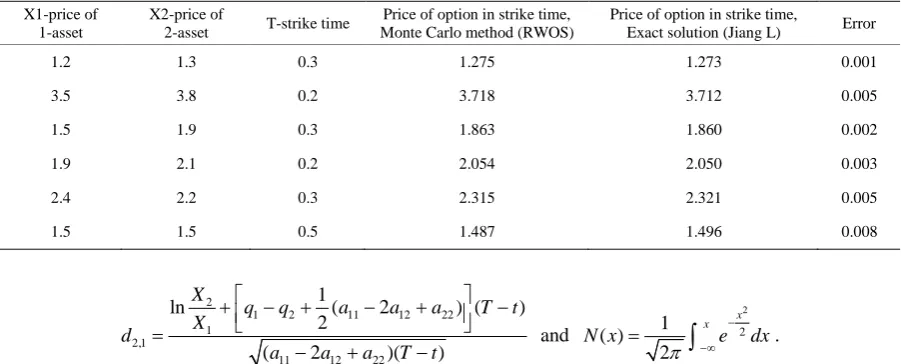
Table 1. The results of calculation for two risky assets.

X1-price of 1-asset

X2-price of

2-asset T-strike time

Price of option in strike time, Monte Carlo method (RWOS)

Price of option in strike time,

Exact solution (Jiang L) Error

1.2 1.3 0.3 1.275 1.273 0.001

3.5 3.8 0.2 3.718 3.712 0.005

1.5 1.9 0.3 1.863 1.860 0.002

1.9 2.1 0.2 2.054 2.050 0.003

2.4 2.2 0.3 2.315 2.321 0.005

1.5 1.5 0.5 1.487 1.496 0.008

2

1 2 11 12 22

1 2,1

11 12 22

1

ln ( 2 ) ( )

2

( 2 )( )

X

q q a a a T t

X d

a a a T t

 

+_ − + − + _ −

 

=

− + − and

2

2

1 ( )

2

x x

N x e dx

π

− −∞

=

_∫

.

Now we will give numerical results which were obtained by the method which is given in [3] and compare with exact solution (2.4).

The results of numerical experiments are given below in Table 1. The number of trajectories (quantity of trails) N = 10,000.

4. Conclusion

Interest in use of Monte Carlo methods for option pricing is increasing because of the flexibility of the method in handling complex financial instruments. Further, the use of variance reduction techniques along with the greater power of today’s workstations has reduced the execution time required for achieving acceptable precision. Monte Carlo simulation will continue to gain appeal as financial instruments become more complex, worksta-tions become faster, and simulation software is adopted by more users. The computational experiments de-scribed above shows that proposed Monte Carlo the algorithms (“random walk on spheroids”, “RWOS”) which was constructed in [1] worked well. In a future we should compare the complexity of proposed in this work al-gorithm with the methods which is given in the paper [2] and find out optimal one.

References

[1] Rasulov, A.S., Mascagni, M. and Raimova, G. (2006) Monte Carlo Methods for Solution Linear and Nonlinear Boun-dary Value Problems. Printing House of UWED, Tashkent. (In English)

[2] Milstein, G.N. and Schoenmakers, J.G.M. (2002) Monte Carlo Construction of Hedging Strategies against Multi-Asset European Claims. Stochastic and Stochastic Reports, 73, 125-157.

[3] Jiang, L. (2005) Mathematical Modeling and Methods of Option Pricing. World Scientific Publishing Co. Pte. Ltd., Singapore.

[4] http://www.investment-and-finance.net/derivatives/m/multi-asset-option.html

[5] http://finmod.co.za/3assetrainbow.pdf