Dynamic GMM Estimation With Structural Breaks An Application to Global Warming and its Causes

Munich Personal RePEc Archive

Dynamic GMM Estimation With

Structural Breaks. An Application to

Global Warming and its Causes.

Travaglini, Guido

Università degli Studi di Roma "La Sapienza"

11 February 2008

Dynamic GMM Estimation With Structural Breaks. An Application to Global Warming and its Causes.

Guido Travaglini

Università di Roma “La Sapienza” Istituto di Economia e Finanza Email: [email protected]

First version. February 2008.

Dedicated to Marta Russo, corruption fighter.

Keywords: Generalized Method of Moments, Multiple Breaks, Principal Component Analysis, Global Warming.

Abstract.

In this paper I propose a nonstandard t-test statistic for detecting n≥1 level and trend

breaks of I(0) series. Theoretical and limit-distribution critical values obtained from Montecarlo experimentation are supplied. The null hypothesis of anthropogenic versus natural causes of global warming is then tested for the period 1850-2006 by

means of a dynamic GMM model which incorporates the null of n≥1 breaks of

1. Introduction.

The literature on the topic of time-series structural breaks has significantly progressed since Perron’s seminal article (1989) that has modified the traditional approach of Unit Root (UR) testing (Dickey and Fuller, 1979). By departing from different null hypotheses that include UR with or without drift, trending series with I(0) or I(1) errors, with or without Additive Outliers (AO), the alternative hypotheses formulated have accordingly included different combinations that range from one single level and/or trend break (Zivot and Andrews, 1992) to multiple structural breaks of unknown date (Banerjee et al., 1992; Bai and Perron, 2003; Perron and Zhu, 2005; Perron and Yabu, 2007).

The present paper, by drawing from this vast experience, and especially from a

seminal contribution in the field (Perron and Zhu, 2005), proposes a novel t-statistic

testing procedure for multiple level and trend breaks occurring at unknown dates (Vogelsang, 1997). This procedure is easy and fast at identifying break dates, as it

compares the critical t statistic, obtained by Montecarlo simulation under the null

hypothesis of I(0) series with stationary noise, with the actual t statistic obtained

under the alternative represented by a I(0) model with a constant, a trend term, the two structural breaks and one or more stationary noise components.

The plan of the paper is the following. Section 2 formulates the theoretical null

and alternative hypotheses maintained, computes the critical values of the t statistics

of the two structural breaks and produces their finite-sample Montecarlo simulations. The Appendix contains some related off-text material.

Section 3 synthetically explains the characteristics and properties of the Generalized Method of Moments (GMM) which is a toolkit necessary to circumvent errors in variables, endogeneity and related problems. Parametric and nonparametric tests for selecting the ‘best’ GMM model specification among alternative sizes of the instrument and regressor sets are introduced and explained, together with the dynamic (i.e. sequential) versions of GMM and of the significance-weighted dynamic Principal Component Analysis (PCA).

Section 4 is addressed at testing a red-hot topic that represents the center stage of many recent top-level discussions: the anthropogenic origin of global warming, supposedly determined by the rapid pace of industrialization and the ensuing worldwide development of productive and commercial activities. The time series of mean World temperatures and of several human and natural forcings for the period 1850-2006 are introduced and then filtered by means of the Hodrick-Prescott procedure (HP). Thereafter, Granger causality and selection of the ‘best’ GMM model specification are performed. Finally, dynamic GMM estimation results

producing the time series of the regression coefficients, their t statistics and the

significance-weighted shares are obtained and exhibited.

2.1. Testing for Structural Breaks. The Null and the Alternative Hypotheses.

The departing point to test for the existence of structural breaks in a time series function is the null hypothesis given by the I(0) series

1) Δ ≡ −y_t y_t y_t−1 = e_t; y1 =0

where y_t spans the period t = 1, ..., T, and e_t ∼N(0,1) corresponds to a standard Data Generating Process (DGP) with random draws from a normal distribution whose underlying true process is a driftless random walk.

Let the field of fractional real numbers be Λ =

{

λ₀,1−λ₀

}

, where 0<λ₀ <1 is a preselect trimming factor, normally required to avoid endpoint spurious estimation in the presence of unknown-date breaks (Andrews, 1993). Let the true break fraction be

λ∈Λ for 0<λ₀ < < −λ (1 λ₀) and λ₀T ≤λT ≤ −(1 λ₀)T the field of integers wherein the true break date occurs.

Given the null hypothesis of eq. 1, the simplest available alternative is provided by a I(0) series with a constant and a trend, their respective breaks, and a time vector of noise. Specifically, the alternative is represented by an augmented AO model (Perron, 1997), usually estimated by Ordinary Least Squares (OLS). In Sect. 3.1, the alternative will be augmented with a vector of exogenous I(0) series and estimated by GMM to account for heteroskedasticity, autocorrelation and endogeneity.

After trimming for the time interval now set as t=

{

λ₀T,(1−λ₀)T

}

, Δy_t is the endogenous variable such that

2) Δ =y_t μ λ₁( )+μ λ₂( )DU_t( )λ τ λ+ ₁( )t+τ λ₂( )DT_t( )λ +ε λ_t( ); ∀ ∈Λλ

where the ( )λ notation refers to the time-changing coefficients and variables of the dynamic equation estimation. The disturbance ε λ_t( )=I I D. . .(0,σ_ε2) is I(0) with

[

_t( )' _s( )

]

0; ,

E

ε

λ

ε

λ = ∀t s, s≠t (Perron and Zhu, 2005; Perron and Yabu, 2007). The two differently defined unknown-date break dummies DU_t and DT_t are: A) 1(DU_t = t>TB_t), a change in the intercept of Δy_t, (μ μ1− 0), namely a break in the

mean level of Δy_t;

B) (DT_t = −t TB_t)1(t>TB_t), a change in the trend slope (τ τ1− 0), namely a change in

the inclination of Δy_t around the deterministic time trend.

The coefficients μ₀ and τ₀ are the respective pre-change values. As a general rule there follows, from the above notation, that any of the two structural breaks is represented by a vector of integers ∀TB_t ∈

{

λ₀T,(1−λ₀)T

}

(Banerjee et al., 1992).

to unknown-date structural breaks in terms of temporary change(s) in the level of the endogenous variable (the "crash" model). Similarly, case B corresponds to temporary shifts in its trend slope (the "changing growth" model) (Perron 1997; Banerjee et al., 1992; Vogelsang and Perron, 1998). Eq. 2, by using both cases together, is defined by Perron and Zhu (2005) as a “local disjoint broken trend” model with I(0) errors (their “Model IIb”).

In addition, for E

( )

Δy_t ≡0 in eq. 2, E

(

μ λ τ λ ≠₁( ), ( )₁

)

0, i.e. the coefficients are expected not to equal zero. The Appendix demonstrates that E

(

μ λ τ λ =₁( ), ( )₁

)

0 holds only for a non-breaks alternative model, namely, when λ =1.

As usual in the break literature, eq. 2 is estimated sequentially for all λ∈Λ. After dropping the λ notation for ease of reading from the single coefficients, we obtain a time series of length 1 (1+ −λ₀)T of the coefficient vector

[

1 2 1 2

]

ˆ( ) , , ,

β λ ≡ μ μ τ τ which is closely akin to the Kalman filter ‘changing coefficients’ procedure. As a by-product, the t statistics of ˆβ λ( ) for the same trimmed interval are obtained and defined as tˆ ( )_μ λ _t and ˆ ( )t_τ λ _t, respectively. They are nonstandard-distributed since the corresponding breaks are associated to unknown dates and therefore appear as a nuisance in eq. 2 (Andrews, 1993; Vogelsang, 1999).

These t statistics can be exploited to separately detect time breaks of type A and/or of type B, just as with the nonstandard F, Wald, Lagrange and Likelihood Ratio tests for single breaks (Andrews, 1993; Vogelsang, 1997, 1999; Hansen, 2000) and for multiple breaks (Bai and Perron, 2003). However, different from these methods that identify the break(s) when a supremum or weighted average is achieved and tested for (e.g. Andrews, 1993), all that is required is to sequentially find as many

t statistics that exceed in absolute terms the appropriately tabulated critical value for a preselect magnitude of λ.

In practice, after producing the critical values for different magnitudes of λ by Montecarlo simulation, respectively denoted as ( , )t_T λ L and ( , )t_T λ T , any n≥1 occurrence for a given confidence level (e.g. 95%) whereby ˆ ( )t_μ λ _t >t_T( , )λ L and

ˆ ( )_{t T}( , )

t_τ λ >t λ T indicates the existence of n≥1 level and trend breaks, respectively, just as with standard t-statistic testing1.

2.2. Theoretical and Empirical t _statistics.

To achieve this goal, some additional notation is required. Let the K₁-sized vector of the deterministic variables of eq. 2 be X_t =

[

1, ,t DU_t( ),λ DT_t( )λ

]

, and let the OLS estimated coefficient vector be

1

3)

0 0

0 0

(1 ) (1 )

ˆ( ) '

T T

t t t t

t T t

y X X X

λ λ

λ λ

β λ − −

= =

=

∑

Δ

∑

with variance 0 0 1 (1 ) 2 ( ) ' T t t t X X λ ε λ σ λ − − = ⎡ ⎤ ⎢ ⎥

⎣

∑

⎦ . Let also the estimated and the true parameter vector respectively be defined as β λˆ( )≡

[

μ τ μ τˆ ˆ ˆ₁, ,_{1 2},ˆ₂

]

and β*≡ ⎣⎡μ τ μ τ₁*, ₁*, ₂*, ₂*⎤_⎦, such

that the scaling matrix of the rates of convergence of β λˆ( ) with respect to β* is

given by ϒ =_t diag T_⎣⎡ 1/ 2,T3 / 2,T1/ 2,T3 / 2⎤_⎦.

Then, by generating Δy_t according to eq. 1 we have, for 0< <λ 1

4) ˆ( ) *

[

( )

]

1 ( )

L

T T T

−

⎡ ⎤

ϒ _⎣β λ −β _⎦ → Θ λ Ψ λ ,

whereby, for W r( ) a standard Brownian motion in the plane r∈[0,1], the following limit expressions ensue:

5)

1 1

0 0

( ) (1), (1) ( ) ,(1 ) (1),(1 ) (1) ( )

T λ σ W W W r dr λ W λ W W r dr

⎡ ⎛ ⎞⎤

Ψ = _⎢ − − − _⎜ − _⎟⎥

⎢ ⎝ ⎠⎥ ⎣

∫

∫

⎦ and 6) 2 2 3 2 3 (1 ) 1 1/ 2 1

2

(1 ) (2 3 )

1/ 3 2 6 ( ) (1 ) 1 2 (1 ) 3 T λ λ

λ λ λ

λ λ λ λ ⎡ ₋ − ⎤ ⎢ ⎥ ⎢ ⎥ − − + ⎢ ⎥ ⎢ ⎥

Θ = ⎢ ⎥

− ⎢ ₋ ⎥ ⎢ ⎥ ⎢ ⎥ − ⎢ ⎥ ⎢ ⎥ ⎣ ⎦ .

From eq. 4 the limit distribution of the coefficient vector is the same as that reported by Perron and Zhu for Model IIb (2005, p.81), while its asymptotic t statistics are computed as follows:

7) t_T( )λ = Θ_T( )λ −1Ψ_T( )λ

(

Ω_T( )λ

)

1/ 2

8.1)

[

]

1

0 1/ 2

(1) ( )

( , ) 3

(1 )

T

W W r dr

t L

λ λ

λ λ

− =

−

∫

8.2)

1

1/ 2 0

1/ 2 2

(3 1) (1) 2(2 1) ( )

( , ) 3

(1 )(3 3 1)

T

W W r dr

t T

λ λ λ

λ

λ λ λ λ

− − −

=

⎡ − − + ⎤

⎣ ⎦

∫

The empirical critical values of the t statistics are obtained by Montecarlo

simulation2. For select magnitudes of λ running from 0.10 to 0.90, and for a

reasonable sample size (T = 200), the 1%, 5% and 10% finite-sample critical values

of eqs. 8.1 and 8.2 are reported in Table 1. These are obtained after performing N =

10,000 draws of the T-sized vector of artificial discrete realizations of Δy_t of eq. 1.

Each of these realizations is in turn given by the cumulative sum of 1,000 values of

(

)

*

. . . 0,1 1,000

t

y N I D

Δ _∼ with y₁* =0.

Thereafter, the Brownian functionals of eq. 5 are approximated by such sums, which are independently and identically distributed, and eqs. 8.1 and 8.2 subsequently computed. Finally, the critical absolute values are obtained by finding the extremes falling in the 99%, 95% and 90% percentiles together with their 10% upper and lower confidence bands.

From Table 1 the critical values can be seen to achieve minimal absolutes at

λ=0.50 and larger values at both ends of λ. Finally, except for λ=0.50, t_T( , )λ L is

smaller than ( , )t_T λ T by a factor that reaches 1.2 at both ends3.

In addition, the N-draws artificially computed t statistics for given values of λ,

considering positives and negatives, are normally distributed with zero mean and variance given by the squares of eqs. 8.1 and 8.2 with the numerators (excluding the integers) replaced by their own standard error obtained by simulation. These

numerators are respectively denoted as ( , ) _t_T λ L numand ( , ) _t_T λ T num. Their

components, the T-length and N-draws series W(1) and

1

0

( )

W r dr

∫

in eqs. 8.1 and 8.2,

are zero-mean I(0) Gaussian processes. However, independent of λ, the former

exhibits unit variance and the latter a variance close to 1/3, being respectively distributed as a standard normal and as a doubly truncated normal distribution with

2

By construction, the squares of the two t statistics, for given λ, correspond to their respective limit Wald-test statistics. As for the first of them see for instance Bai and Perron (2003). For both see Vogelsang (1999) although the simulation method adopted therein differs from that of the present paper.

3

extremes close to 5% and to 95%. These are the only constant variances, since all the

others are strictly dependent on the magnitude of λ.

The results of the numerators and other statistics are reported in Table 2 with

T=200. The variances of the estimated numerators of eqs. 8.1 and 8.2 achieve a

minimal value at λ=0.50, being more than twofold for the first and more than tenfold

for the second at both ends. Both λW(1) and (3λ λ−1)W(1) grow, as their variances

respectively are λ2 and

(

λ λ(3 −1)

)

2. The variance of the second component of the

numerator of eq. 8.2,

1

0

2(2λ−1)

∫

W r dr( ) , achieves a minimum of zero at λ=0.50 and

rises at both ends. Similarly for the variances of the simulated t statistics (shown in

the last two columns of Table 3), which attain a minimal value in correspondence of

λ=0.50, where they share an almost equal value and then increase by eight and ten

times at both ends, respectively. Finally, the estimated variance of the first statistic is on average 40% smaller than the second, reflecting the similar albeit smaller gap in their critical values, as reported in Table 1.

3.1. The Dynamic Generalized Method of Moments (GMM).

A K₂-sized vector of stationary stochastic components

2

,1,..., ,_K

t t t

X = ⎣⎡x x ⎤_⎦ is

now introduced alongside with the vector of deterministic components X_t described

in Sect.2.2. X_t may include contemporary and/or 1≤ H <T lags or leads of their

observations. Together with X_t, it constitutes the entire K-sized vector of regressors

X_t = ⎣⎡X X_{t t}⎤_⎦, whereK =K₁+K₂.

Eq. 2, in an OLS setting, can thus be extended to produce the following dynamic estimating equation:

9) Δ =y_t X_tB( )'λ +e_t( )λ

where

1

1 2 1 2 1

( ) , , , , ,..., _K

B λ = ⎣⎡μ μ τ τ ξ ξ ⎤_⎦ and ξ_k, k =1,...,K₂, are the coefficients of X_t,

∀λ ∈Λ. Finally, e_t( )λ =I I D. . .(0,σ_e2).

Eq. 9, just as eq. 2, enables constructing a time series of length 1 (1+ −λ₀)T of

the coefficient vector ( )B λ and of the ensuing two t statistics ˆ ( )t_μ λ _t and ˆ ( )t_τ λ _t4.

GMM estimation of ( )B λ requires the introduction of an L-sized Z_t instrument set

(

L≥K

)

. In many cases, Z_t is represented by lag transformations of the set X_t such

that Z_t = ⎣⎡1,X_{t m−} ⎤_⎦, for m=1,...M lags and 1≤H ≤M <T .

4

The L-sized vector of sample moments for the trimmed time interval is 10) 0 0 (1 ) ˆ _ˆ ( , ) ( ) T

t t t

t T

g Z e

λ

λ

β λ − λ

=

=

∑

where the coefficient vector ˆβ and the first-stage residuals eˆ_t stem from a (possibly)

consistent TSLS estimation of eq. 9. The sample means of the above are

[

]

1

0

ˆ ˆ

( , ) (1 ) _t( , )

g β λ = −λ T − g β λ

with the orthogonality property thatE g⎡_⎣ (βˆ_t)⎤ ≡_⎦ 0.

Let also the ensuing L L× weight matrix be

11) 0 0 (1 ) 1 0

ˆ ˆ ˆ

( , ) (1 ) ( , ) ( , ) '

T

t t

t T

W T g g

λ

λ

β λ λ − − β λ β λ

=

⎡ ⎤

=_⎣ − _⎦

∑

such that ˆ_GMM( ) arg min

(

g( , )ˆ W( , )ˆ 1g( , )ˆ

)

β

β λ β λ β λ − β λ

∈Β

= .

Computation of the partial first derivatives of the sample moments yields the

L K× Jacobian matrix

12) 0 0 (1 ) 1 0

( ) (1 ) '

T

t t t

t T

G T z x

λ

λ

λ λ − −

=

⎡ ⎤

= _⎣ − _⎦

∑

where , z_t x_t respectively are the L.th and the K.th element of vectors Z_t and X_t.

Finally the efficient GMM estimator, by letting

0 0 (1 ) ' T t t t T

Z y z y

λ

λ −

=

=

∑

Δ is

13) βˆ_GMM( )λ = ⎣⎡G_t'( )λ W( , )β λˆ −1G_t( )λ ⎤_⎦−1G_t'( )λ W( , )β λˆ −1Z y' _t

where, specifically

14)

1

1 2 1 2 1

ˆ _{( ) ˆ ˆ, , , , ,...,ˆ ˆ} ˆ ˆ

GMM K

β λ _{= ⎣}⎡μ μ τ τ ξ ξ ⎤_⎦

whose asymptotic normality property is

(

)

1/2 ˆ * ˆ

( ) N 0, ( , )

d GMM

where

15)

0 0

1 1

(1 ) (1 )

ˆ ˆ

( , ) T '( ) ( , ) T( )

S G W G

λ λ

β λ λ β λ − λ −

− −

⎡ ⎤

= ⎢_⎣ ⎥_⎦

is the “sandwich” matrix.

The reasons for selecting a GMM estimation model in the present context are the following:

1) the model perfectly suits the I(0) model of eq. 2 so that the estimated relevant t

statistics are easily comparable to their simulated critical values of Table 1;

2) the estimated coefficients are scale-free relative to equations in levels as the regressors in origin are often differently indexed with the risk of producing, otherwise, spurious coefficient results;

3) GMM estimation automatically corrects for autocorrelation and heteroskedasticity of the error term by using the Heteroskedasticity and Autocorrelation Consistent (HAC) method (Newey and West, 1987);

4) By accordingly selecting the optimal instrument vector, GMM disposes of parameter inconsistency deriving from error-in-variables estimation.

In particular, the second point implies the fact that nonstationary series, unless

cointegrated, produce spurious coefficient t statistics, error autocorrelation and a

bloated 2

R (Granger and Newbold, 1974; Phillips, 1986). Spuriousness is also found

between series generated as independent stationary series with or without linear trends and with seasonality (Granger et al., 2001) or with structural breaks (Noriega and Ventosa-Santaulària, 2005). These occurrences are found in this literature with

OLS regressions where the t statistics – in particular those of the deterministic

components – diverge as the number of observations gets large5.

In the context of Instrumental Variables regressions with a stationary

endogenous variable, however, spuriousness of the coefficient t statistics arises when

many instruments and/or a large bandwidth are used. This is the reason why the appropriate bandwidth and number of instruments must be chosen (Koenker and

Machado, 1999; Hansen and West, 2002; Kiefer and Vogelsang, 2002) 6.

5

By means of some applied experimenting with Montecarlo simulation, it is shown that in a standard OLS (T=200) model with an I(0) endogenous variable and T≥K≥1regressors, the t statistics of the coefficients of the deterministic components, by departing from values below unity at K=1, diverge toward a value of 2.00 at a rate of K1/ 6. With an I(1) endogenous variable, the same t statistics depart at K=1 from values over 8.0 and 15.0 for the constant and the trend, respectively, and remain virtually unchanged with increasing K.

6

In a setting characterized by an I(0) endogenous variable, selection of the appropriate HAC bandwidth (HB) and number of instruments (L) is crucial, since large values of both give rise to spurious t statistics of the regressor coefficients and of their higher-fractile values. In fact, by means of the same kind of applied experimenting as the above, it is found that for T=200,three regressors (constant, trend and a stationary variable) and select HB = 0,1,5,30, the t statistics grow respectively at rates 1 5 1 4 1 3

, ,

L L L and _L1 2

, and in general _L1 2

3.2. Parametric and Nonparametric Tests for the Selection of Alternative GMM Models, and Dynamic Principal Component Analysis.

In GMM modeling of the static version of eq. 9, the researcher is faced with a large variety of choices regarding the size of the regressor and instrument sets

(provided L≥K), especially when lags and/or leads of these can be included. In fact,

coefficient estimates and their efficiency and significance can be very sensitive to different choices (Hansen and West, 2002). The search for the ‘best’ or ‘optimal’ model specification is thus no easy task, since it is based on a careful weighting procedure among a batch of selection tests.

These tests are applicable to the static version of eq. 9, namely, to the single regression that covers the sample time span. Since this regression provides a mean of

the coefficients and statistical tests of all the regressions for λ∈Λ, the appropriate

selection can be easily performed. The most commonly used model selection tests fall into two categories: parametric and nonparametric, as follows

1) the Akaike and Schwarz Criteria (AIC and BIC) utilized to select optimal lag length of the regressor set;

2) the Durbin-Watson (DW) test for first-order autocorrelation;

3) the J statistic for overidentifying restrictions (Hansen, 1982), distributed as χ2_{L K−} ; 4) the Anderson-Rubin (AR) and the LM tests for TSLS instrument weakness

proposed by Andrews and Stock (2007), respectively distributed as F_{L T L, −} and χ2_L.

5) the minimum eigenvalue (MIE) of the HAC weight matrix W( )βˆ to assess its magnitude, i.e., the closeness to zero (orthogonality) of the GMM sample moment means g_t( )βˆ ;

6) the MIE of the T-scaled sandwich matrix S( )βˆ (eq. 15), to test for the magnitude of the variance of eq. 9, that is, for model efficiency;

7) the maximum eigenvalue (MAE) of the matrix X Z Z Z_t' _t

[

_t' _t

]

−1Z X_t' _t, to test for first-stage TSLS instrument size reduction;

8) the MIE of the first-stage TSLS matrix which, for Ω =e e_t' _t, is defined as

[

]

1

1 1

G_T = Ω− X Z Z Z_t' _{t t}' _t − Z X_t' _tΩ− , a slight variant of the weak-instrument testing proposed in the literature (Stock et al., 2002; Stock and Yogo, 2003);

The first, rather than parametric, may be defined as a scoring test, while the other three are parametric with known distributions. Instead, the eigenvalue-based tests and their implied null hypothesis are typically nonparametric and require some explanation. Specifically, the first three eigenvalue tests (5 to 7) stem from central Wishart ensembles whose entries derive from Gaussian series N I D. . .(0,σ2). These ensembles are real p.d. symmetric covariance or correlation matrices, here denoted as

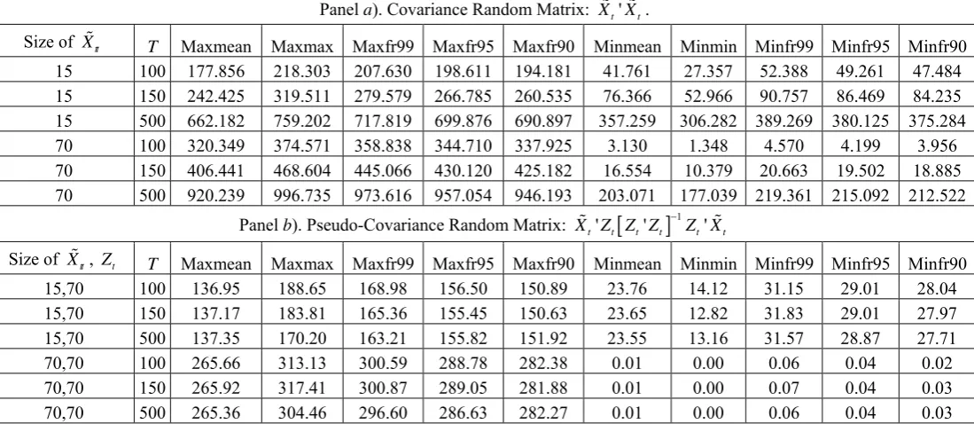
Critical values of the latter are supplied by the authors, while those of the former are exhibited in Table 3 for N.I.D.(0,1) and sample series of different sizes, 15 and 70, chosen to accommodate the actual samples used in this paper, and lengths (T=100, 150 and 500). N=1,000 Montecarlo draws for each simulation were used. V

is a standard covariance matrix in the first two cases (5 and 6) and a pseudo-covariance in the third (7)7. For this purpose, Panels a and b are respectively exhibited in Table 3.

For V a covariance or correlation matrix originated from N I D. . .(0,σ2) series, the bulk spectrum (screeplot) limiting joint distribution of the sample eigenvalues is close to normal if K₂ is small, and converges to the Marčenko-Pastur distribution as

2

K gets larger (Johnstone, 2001). Moreover, the sample mean of the eigenvalues is T

(unity) if V is a covariance (correlation) matrix, independent of K₂ and T. Instead, the limiting joint distribution of the centered and scaled MAEs follows the left-skewed Tracy-Widom joint distribution (Johnstone, 2001; Tracy and Widom, 2002), while the limiting joint distribution of the centered and scaled MIEs is usually very close to normality8.

In random matrix theory, the MIE is of particular relevance to establish the ‘magnitude’ of a matrix when the MAE→ ∞ whereby no precise guidance could be supplied in the field of indefinite numbers. The MAE is of equal relevance, especially when the MIE →0, although it addresses a different target by catching, together with the corresponding eigenvector, a larger if not most part of the variations of the bulk of the components of V.

Both eigenvalue-based tests are used for comparative purposes among different models and entail specific null hypotheses. In fact, the null hypothesis of the MIE is that of no conditioning of the entire vector of components (i.e. instrument weakness), while the null hypothesis of the MAE conforms with size reduction of PCA. By consequence, for a preselect significance level, a MIE (MAE) larger than the critical value of Table 3 rejects no bulk conditioning (no size reduction).

Given X_t (Sect. 3.1), define by virtue of the Spectral Decomposition Theorem

the symmetric covariance matrix X X_t' _t =ERE, where R is the K₂×K₂ diagonal matrix of the eigenvalues r_i , (i=1,...,K₂) in descending order, and E the same sized matrix of eigenvectors with column elements v_{i j,} , (j=1,...,K₂). For each jth eigenvector E_j, define the scalar v_m =arg max(E_j), (m=1,...,K₂; m≠i) such that the

7

The matrix X Zt' t is rectangular insofar as L>K2. Hence the eigenvalues of the matrix [ ] 1

' ' '

t t t t t t

X Z Z Z − Z X are not the same as those of a standard random square matrix, because they are independent of T as shown in Table 3. Also, the distribution of the MAEs is somewhat different, as stated in the subsequent footnote.

8

static PCA shares, corresponding to the eigenvalues in descending order, are described as follows

16)

2

1

( | ) K

i i m i

i

s r v r

=

=

∑

.

After defining α_m the mth. regressor’s marginal significance of the coefficient, the time series of length 1 (1+ −λ₀)T of the mth. regressor’s dynamic and significance-weighted share measured over the trimmed interval t∈

{

λ₀T,(1−λ₀)T

}

may be expressed as

17)

( )

( )

2

1

(1 ) ( | ) ; K

i m i m i

i

s r v r

=

⎡ ⎤

λ =_⎢ − α _⎥ λ ∀λ∈Λ

⎣

∑

⎦ ,

which provides the Dynamic PCA to be exploited in the following Sections.

Apart from the dynamics involved, eq. 17 is preferable to eq.16 because it weighs each component share by the statistical significance appended to its coefficient. Traditional PCA, in fact, by ignoring this evidence and by sticking to nominal shares, may overstate in quite a few instances the components whose role is virtually close to zero.

4.1. Global Warming and Forcings During the Period 1850-2006.

Planet Earth has passed through many waxing and waning climate episodes during the entirety of its life. For instance, the Mid-Cretaceous (120-90 million years ago) and the Paleocene-Eocene Thermal Maximum (PETM, 55 million years ago) have experienced temperatures distinctly warmer than today, with animals and plants living at much higher latitudes and with higher carbon dioxide (CO2) levels, roughly two to four times than the present-day ones.

Abrupt climate changes have occurred also during the more recent Phanerozoic eon (Shaviv and Veizer, 2003), like the last glacial period (Alley, 2000), the Medieval Warm Period, centered around 1000 A.D., and the Maunder Minimum in Europe during the years 1645-1715 A.D. Many of these changes have affected human activities, like the disappearance of the Neanderthal man and countless population migrations, e.g. the Siberian exodus toward the Americas, the Dravidian occupation of Ceylon, and the short-lived experience of the Vikings in Greenland.

of Northern Africa, partly commenced since the late Roman Empire and that of Australia, caused by extensive burn-and-slash practices of the aboriginals.

While the above cited may be casual episodes of the often perverse relationship between humans and nature, the by now secular global warming phenomenon is undoubtedly cause of concern. In fact, the last hundred years or so have experienced a renewed climate change by exhibiting a rise in the mean global surface temperature by about 0.6 ± 0.2°Csince the late 19th century, and by about 0.35 ±0.05° C over the last 40 years (Chenet et al., 2005). This global warming phenomenon, while definitely not being unique in Earth’s history (Baliunas and Soon, 2003), has spurred intense debate on the analysis of its causes and is by now a worldwide major issue which involves popular media, scientists, corporations, governments and political organizations.

In fact, while the rise in temperatures is of undisputed evidence, yet at a lower pace in the last decades, the search for a main culprit is still in progress and well alive, and is being characterized by two opposing fronts regarding its causes: the advocates and the skeptics of the anthropogenic origin.

Advocates of the human-induced greenhouse effects, purportedly caused by CO2 emissions and industrial aerosols, include several scientists (e.g. Hansen et al., 2007), the UN-mandated Nobel-prized Intergovernmental Panel on Climate Change (IPCC), and large sections of governments and politicians, involved in fostering public scares, fund raising, propaganda, data mining and even red tape9.

Skeptics, on the other hand, form a scientifically-based consensus that supports and proves the prevalence of long-run evolving natural causes, defined as “global forcings”, like solar activity and Cosmic Ray Flux (CRF) (Shaviv and Veizer, 2003; Svensmark, 1998; Bard and Frank, 2006, Usoskin et al., 2003), volcanic aerosols (Mann et al., 2005) and ocean currents (Gray et al., 1997). This consensus is based on reliable paleoclimatological dataset reconstructions (e.g. Crowley, 2000; Lean, 2000, 2004; Usoskin et al, 2003, 2004a, 2004b; Mann et al., 2005; Krivova et al., 2007), most of which are downloadable from the National Oceanic and Atmospheric Administration (NOAA) website.

Clearly, the analysis of the interaction of the variables implied in the secular global warming process is very complex, as it requires countless and valuable in-depth experimenting stemming from different scientific fields, such as astrophysics, climatology, biology and chemistry. Statistics and econometrics may contribute to the current state of knowledge by supplying interesting insights into causality occurring in a casual environment. Not much work has been produced hitherto in this field, except for few though valuable contributions (e.g. Lanne and Liski, 2004; Kaufmann et al., 2006). Certainly more will come in the future.

9

Global warming is identifiable with data sets on land and sea temperature recordings collected by different agencies for select periods, areas, altitudes, hemispheres, etc. Of these, the Best Estimated Anomaly (BEA) of the updated HADCRUT3 dataset (Brohan et al., 2005), available for the period 1850-2006 on an annual basis, was here selected due both to its spatial and temporal breadth. Therefore, the BEA index represents the endogenous variable used in eq. 9, whose GMM estimated parameter vector is given by eq. 13.

In line with BEA, which constitutes a time series of 157 observations and is synonym of global warming and climate change10, an ample dataset of forcings was retrieved from different sources worldwide available over the internet, and especially from the NOAA website. The list of forcings which play the role of regressors and instruments in GMM estimation is exhibited in the Data Description and Sources, and is made of the following two main categories: anthropogenic and natural forcings.

The anthropogenic forcings include average real GDP percapita of the total 12 Western Europe major countries and of its overseas offshoots (U.S.A., Canada, Australia and New Zealand), and their total population (Maddison, 2007)11. They are respectively labeled INCOME and TPOP. Anthropogenic forcings also include the components of trace or greenhouse gases (GHGs), which are given by four measures of emissions: carbon dioxide in global volume (Marland et al., 2007), and final emissions of CO2, methane and nitrous oxide expressed in terms of Radiative Forcing (RF) (Robertson et al., 2001). They are respectively labelled as: CO2V, FCO2, FCH4 and FN2O. While the first may be considered as a stock, the other three are a flow.

The category of natural forcings includes the average yearly number of monthly sunspot series (NGDC, 2007), a measure of total solar irradiance received at the outer surface of Earth's atmosphere in terms of RF (Krivova et al., 2007), combined solar and volcanic RF, composite solar RF, combined solar and volcanic RF, composite volcanic RF, tropical volcanic RF (Mann et al., 2005) and, finally, Pacific Decadal Oscillations (Shen et al., 2006). In sequence, these forcings are labelled as: SUNSPOTS, TSI, VOLSOL, COMPSOL, COMPVOL, VOL and PDO.

When unavailable for the more recent years, the data series are forecasted by the autoregressive method, with lags p selected via minimum BIC. Other available data, such as tropical solar RF (Mann et al., 2005), tropospheric aerosols represented by sulphur and fossil-fuel black carbon emissions (Crowley, 2000), and measures of Beryllium 10 (10Be ) and Radiocarbon 14 (14C ) that proxy CRF (Crowley, 2000), were left out of the list because of excess collinearity with some of the above. In fact, after performing appropriate HP filtering (Hodrick and Prescott, 1997) of all level forcings – logged when applicable12 – and extracting their cyclical component, these

10

On the subtle, yet not insignificant difference between climate and temperatures see Baliunas and Soon (2003).

11

By dating back to 1850, this data subset - albeit limited - is the only available in Maddison’s comprehensive statistics that stretches the period chosen.

12

were found to be correlated at levels higher than 0.85, and then discarded because of the risk of obtaining downsized coefficients and t statistics during regression estimation.

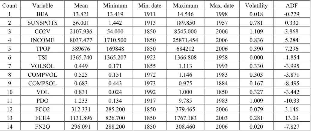
Table 4 reports some descriptive raw statistics of BEA and of the 13 selected forcings. Of interest are the large differences between the minima and the maxima of SUNSPOTS, PDO and CO2V, expressed in terms of their volatility coefficients. Also, the majority of the ADF t-test statistics reveals nonstationarity, justifying the need for filtering in order to achieve nonspurious regression results (Sect. 3.1).

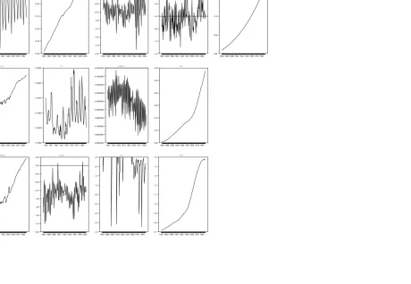
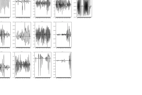
Finally, Figs. 1 to 3 illustrate the levels and the HP-filtered differences of the logs of BEA and of the 13 forcings. From the left panel of Fig. 1, global warming can be shown to exhibit a trending behavior since 185013, which is ostensibly stationary when appropriately differenced. All of the human forcings exhibit a trend, but methane (FCH4) seems to taper off in the last decade. On the other hand, the natural forcings are mostly cyclical, with SUNSPOTS exhibiting a known regularity of around 11 years.

While retaining their labels, all the variables used in calculations and estimations that will follow are henceforth understood, unless otherwise defined, to be represented by their HP-filtered magnitudes (see fn. 12).

4.2. Expected Effects of Forcings over Global Warming.

The 13 listed forcings by means of ongoing research are expected to bear specific effects over the World temperature changes represented by BEA. Whether founded or ungrounded, these purported effects are at first presented, then tested for by means of Granger causality testing (Granger, 1969).

Of the human forcings, economic activity and the size of population (INCOME and POPULATION) are expected to raise BEA via GHG emissions, extensive deforestation and generalized use of inefficient technologies. The United States and China nowadays, appear by some estimates to be the main responsible for CO2 volume emissions, and especially the second is poised to double its GHG emissions within a decade or so.

Solar activity manifests itself in different forms that may significantly affect climate variability. Sunspot numbers (SUNSPOTS), total solar irradiance (TSI) and solar cosmic rays (CRF) are highly correlated and constitute the ensemble of “solar forcing”. Their long-run reconstructions stem from direct measurements, like the

cyclical nature (e.g. sunspots). Too low a smoothing parameter applied to low-frequency raw series would in fact produce a cyclical output not strictly comparable with that obtained from high-frequency raw series, thereby giving rise to spurious coefficients in regression estimation.

13

The logged level of the BEA equation can best be represented as follows

4 6 2 2

1

(BEA) 1.103-10 10 .578 (BEA) ; R .829, D.W.=1.981 (6.4) (2.1) (3.9) (8.8)

t t

Log = −T− −T + Log ₋ =

where the t-statistics are reported in brackets, and T and 2

sunspot numbers since Galileo, or from solar proxy variables like the accumulated layers of 10Be in ice cores and 14C in tree rings. Whether directly or through cloud formation or by changes in the Earth’s albedo, solar forcings are in many cases shown to sizably affect the Earth’s climate (Usoskin et al., 2003, 2006; Shaviv and Veizer, 2003; Svensmark, 1998).

In particular, increased sunspot activity – according to some theories – causes a cooling of the Sun’s surface by trapping its energy output. This was evidenced by telescope measurements made from 1976 to 1980, which showed that the sun's surface had cooled by about 6° C as the number and size of sunspots increased. Also, it is known that the Little Ice Age coincided with a sunspot minimum. However, the matter is debated, since according to other theories the correlation between climate changes and sunspot numbers is positive (Baliunas and Soon, 2003).

TSI is expected to raise the Earth’s temperatures via increased luminosity, although there is no general agreement on its size and significance nor on its relationship with sunspots, since its variability (only 0.1%-0.2% over the 11-year cycle) is so low as to deserve the nickname of ‘solar constant’ (Fouka et al., 2006). TSI is likely to operate in conjunction with the CRF by negatively affecting climate via low-altitude cloud cover and increased rainfalls (Svensmark, 1998; Svensmark and Frijs-Christensen, 2007; Shaviv, 2005).

Volcanic activity is also poised to affect climate, especially in the Northern Hemisphere (Shindell et al., 2004). The release of aerosols rich of sulphates and CO2 reflects sunlight away from the surface of the Earth causing a climate cooling due to dust veils (tephra) suspended in the atmosphere. At the same time, however, aerosols absorb solar and infrared radiation leading to warming of the surrounding air masses. This applies in particular to large volcanic eruptions whose effects may last for years, as in occasion of the eruptions of Krakatoa in 1883, El Chichón in 1982 and Pinatubo in 1991. The net effect on overall climate is therefore still matter of dispute (Shindell et al., 2004; Mann et al., 2005; Chenet et al., 2005).

The IPCC doggedly defends since at least a decade the anthropogenic hypothesis by stating in its Third Assessment Report (AR3 2001) that "forcing due to changes in the Sun's output over the past century has been considerably smaller than anthropogenic forcing…Its level of scientific understanding [is] very low, whereas GHGs forcing continues to enjoy the highest confidence level….[and] the temporal evolution indicates that the net natural forcing has been negative over the past two and possibly even the past four decades….[It is thus] unlikely that natural forcing can explain the warming in the latter half of this century".

energy within the troposphere14.

The contentions here produced can be on a first instance checked by means of Granger Causality testing, which uses a regression of the following kind:

18) _{, , , t}

1 1

+ +

P P

i t p i t p p j t p

p p

X a θ X ₋ ϑ X ₋ υ

= =

= +

∑

∑

where a is the constant term, and υ_t is an IID disturbance. X_{i t,} is the preselect forcing

regressed against a constant, lags of itself and lags of a preselect cross forcing X_{j t,} ,

i≠ j. The parameters θ_p and ϑ_p refer to their own arguments for lags p∈[1, ]P .

After setting a range of P from 1 to 35 years, the BIC is chosen as the proper

lag selection criterion, since for small samples the AIC – by prefering longer lags – is notoriously inconsistent. Results of the most relevant causalities are exhibited in Table 5, with the proviso that they are merely descriptive being of bivariate nature and that only multivariate econometric modeling, especially in the dynamic form adopted in this paper, provides the necessary guidance for drawing grounded conclusions regarding causality.

Specifically, the only significant Granger causalities (beneath 5% marginal significance) are those recorded from TSI to SUNSPOTS, which is negative, and those from volcanic activity and PDO over BEA, which respectively are positive and negative. Apart from these, no causality is acceptable by common standards, excluding the one running from CO2V to BEA (which stands beneath 10% marginal significance and is positively signed). Far from drawing from this evidence hasty and unwarranted conclusions, the long-debated IPCC contention finds some support, let alone the results emerging from the following Section.

4.3. GMM Model Selection and Preliminary Empirical Results.

As advanced in the Introduction, testing for breaks in the time series of global warming and its causes is equivalent to testing for the null hypothesis of its anthropogenic nature. Natural causes during the period 1850-2006, in fact, do not exhibit any known substantial break worldwide.

The detection of single and multiple breaks, obtained by means of the Zivot- Andrews (1992) and of the Bai-Perron (2003) procedures, produces conflicting results which are very sensitive to both the lags of the endogenous variable and of the

forcings included15. This is an additional reason for proceeding, after performing the

14

According to some IPPC estimates, “a GHG level of 650 ppm would “likely” warm the global climate by around 3.6°C, while 750 ppm would lead to a 4.3°C warming, 1,000 ppm to 5.5°C and 1,200 ppm to 6.3°C. Future GHG concentrations are difficult to predict and will depend on economic growth, new technologies and policies and other factors” (Press conference, Paris, February 2, 2007)

15

optimal static GMM model selection, along the lines of the proposed dynamic method so as to analyze the time series of breaks, coefficient and shares of the forcings that determine global warming.

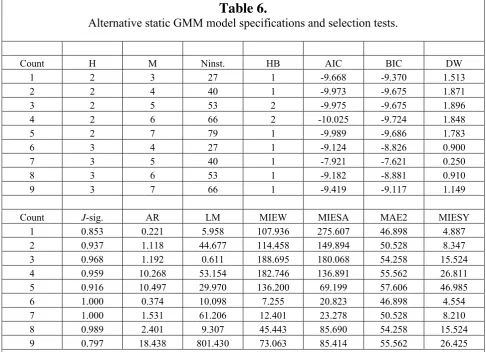
Table 6 shows, with reference to Sect. 3.2, the magnitudes of the different tests

adopted to select the optimal H/M combination among different static GMM model

specifications16. While the magnitude of the Durbin-Watson statistic (DW) definitely

rules out H=3, the AR and especially the LM test statistic (Andrews and Stock,

2007) significantly point to the combination H=2 and M=6, for a size of the

instrument set L=66 and a HAC bandwidth (HB) equal to 2. DW, the AIC and BIC

also prefer M=6 with respect to M=7.

In addition, the first two MIE tests for H=2 included in Table 6 exceed the 99%

critical values reported in Table 3 Panel a for similar sizes, thereby rejecting the null

of no weakness, so much as the last MIE test, whose magnitude exceeds its critical value (Stock et al., 2002; Stock and Yogo, 2003). Finally, the MAE test statistic falls

short of the corresponding tabulated values in Table 3 Panel b, significantly not

rejecting the null of no size reduction.

Finally, the combination of the MIE and MAE with the AIC and BIC results

lend support for the optimal H/M parsimonious combination to be made up of 2

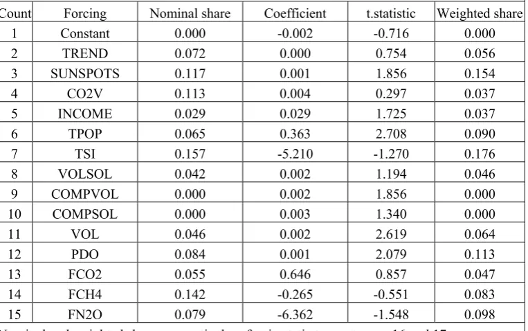
regressor and 3 instrument lags, for a size of the instrument set L=66. Table 7 shows

the coefficient and share results of the corresponding static GMM specification. The shares reported are both expressed in nominal and in significance-weighted terms. As to the latter, the sum of the natural and of the human forcing contributions respectively are roughly 55% and 35%, well off the mark of 10% and 90% established by the IPCC (AR4, 2007). Interestingly enough, when passing from nominal to weighted shares, the contribution of CO2V dramatically falls while that of FN2O slightly rises.

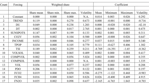
Table 8 eventually produces the statistics of the dynamic GMM estimation

with breaks. Due to a trimming factor λ =₀ .10, the period covered is restricted to

1864-1990. The weighted share means reported17 assign to the trend and to changes

in the major natural forcings (SUNSPOTS, TSI and PDO) a tally of over 70%. Only one of the weighted shares of changes in the anthropogenic forcings exceeds 5%, and their tally is no more than 20%. In particular, the share of CO2 volume emissions is responsible of climate changes in terms of global warming by 5.6% only, well far away from the 90% statistic concocted by the IPCC (AR3, 2001).

The mean coefficients are also of interest. Changes in TSI, FCO2 and FN2O have a negative effect over climate changes independent of their magnitude, which reflects the different scales of the forcings (see Table 4). Hence, they are on average

16

The combination H=3 and M=8 is not included due to some matrix singularities. With H=1, the statistical significance of the J statistics is unacceptably low and its results go unreported. Finally, larger H magnitudes than those reported exceedingly reduce the degrees of freedom given the length of T. The repetition of the “Count” column in the Table is merely included for readability purposes. Although unreported for ease of space, the ADF t-test statistics of the disturbance significantly reject the null of no stationarity.

17

temperature dimmers. There follows, thus far, that two out of three GHGs expressed in RF do not cause warming, but on the contrary prevent solar irradiance to reach the Earth’s surface.

In addition, changes in TSI on average are dimmers while SUNSPOTS are warmers. This counterintuitive evidence can be explained by the recently reckoned phenomenon that solar flares, which occur to the accompaniment of TSI, generate storms of solar-magnetic flux that partially shield the Earth from cosmic radiation and promote cloud formation (Svensmark, 1998; Svensmark and Frijs-Christensen, 2007). On the other hand, sunspot numbers are on average warmers because, by raising total solar output, they negatively affect mean cloudiness and outweigh the

effect of TSI (Baliunas and Soon, 2003; Usoskin et al., 2003).

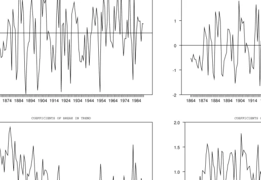
4.4. Time Series of Breaks, Coefficients and Shares of the Selected GMM Model.

Of even greater interest than the results above reported is the analysis of the overtime evolution of breaks, coefficients and weighted shares obtained from the selected dynamic GMM model estimation.

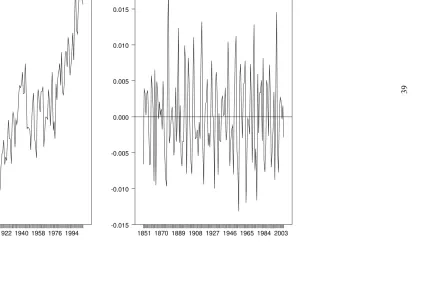
Fig. 4 shows the time series of the coefficients and of the t-statistics of the level

and trend breaks. Neither of these exceeds in absolute terms the critical values

provided in Table 1 for any of the given λ magnitudes. In fact, their minima

(maxima) respectively are -1.897 and -0.415 (2.754 and 1.775), well within the absolute value of any of the tabulated figures. The purported null hypothesis of one or more structural breaks associated to human forcings is therefore rejected, different from the results previously achieved with the Zivot-Andrews and the Bai-Perron tests (Sect. 4.3), and similar in kind to those of Lanne and Liski (2004).

The trimmed time series of the level and trend break coefficients are shown in Fig. 4. The first exhibits no trend and has a nonzero mean, while the second has zero mean and is slightly declining with time, i.e., it has a negative trend. This reinforces the finding that the endogenous variable (BEA) tapers off overtime, as shown in Sect. 4.1.

Fig. 5 shows the time series of the coefficients of the individual forcings, whose descriptive statistics are provided in Table 8. For most part of the trimmed sample, the impact of changes in the GHGs (FCO2, FCH4 and FN2O) over BEA is of negative sign, confirming their dimming as opposed to warming effect over climate changes. Only the impact of the CO2 volume is mostly positive, but it shows a severe drop since the second half of the Seventies, perhaps because of the improved worldwide controls over its emissions (Lanne and Liski, 2004). In any case, the sign positiveness of CO2V is explained by condensation of FCO2 emissions into clouds and aerosols formed by their cooling of the troposphere. This accumulative process after several decades, by absorbing solar infrared energy, causes like volcanic activity a greenhouse effect (Hansen et al., 2007) and/or a magnified transmission of solar irradiance over the Earth’s surface.

positive and negative in sign, respectively. Their patterns are somehow specular in trend, since the first peaks in the years 1940-50 and the second troughs a decade later. Specifically, the coefficient of SUNSPOTS has been falling during the last half-century or so, while that of TSI has been rising. While retaining the conclusion that the first variable is a warmer and the second a dimmer, the net dynamics of the coefficients are consistent with the tapering off of BEA, which is demonstrated to be caused by a reduced impact of sunspot activity and a growing impact of solar irradiance. Of varying intensity, and positively signed, are also the coefficients that represent the impact of volcanic activity (VOL) and of the Pacific Decadal Oscillation (PDO) over climate changes. While VOL’s ‘winter warming’ impact (Shindell et al., 2004) is falling since the early 20th. century after the Krakatoa effect, the PDO’s impact is widely cyclical, but exhibits a drop during the last decades (Gray et al., 1997).

Since the coefficients of other forcings are mostly irrelevant, there remains to interpret the time-changing effects, both positively signed, of the remaining two anthropogenic forcings: incomes and total population. INCOME’s impact over BEA shows a dramatic drop since the early sixties, maybe because of the large introduction of more efficient techniques and of the progressive abandonment of coal as a source of energy. It again rises since the early Nineties in conjunction with TPOP’s impact, maybe because of the large-scale industrialization process enjoyed by China and India, where energy consumption is still out of check.

Figs. 6 and 7 show the HP-smoothed composite and individual weighted shares of all forcings obtained by applying the dynamic PCA criterion introduced in Sect.

3.218. While letting the explanatory role of coefficients unabated, the time-varying

shares gauge the size of the contribution of the forcings in the variance of climate changes. In particular, from Fig.6, the share of all solar forcings (SUNSPOTS, TSI, VOLSOL and COMPSOL) unmistakably rises during the trimmed period considered from 28% to nearly 45%, while that of population and incomes more than halves from an initial value of 12%. The other two composite shares, represented by all emission forcings (CO2V, FCO2, FCH4 and FN2O) and by nonsolar natural forcings (VOL, COMPVOL and PDO), remain essentially constant though exhibiting slight troughs within the first third of the trimmed sample. They respectively average 13% and 26%, as computable from Table 8.

In Fig. 7 the evolution of the individual weighted shares is shown. Of special interest are those of SUNSPOTS and TSI, VOLSOL and COMPVOL, all on the rise. The last of these compensates the falling VOL’s share so as to safely conclude – even more so after adding the contribution of VOLSOL – that the major volcanic eruptions during the period considered (Krakatoa, Mount St.Helen’s, Pinatubo and a few more) have played a significant role in global warming, although with an overtime falling effectiveness as previously observed.

Of the GHGs, all shares are declining except for the share of CO2V, which

18

grows from 2% to 8%. This evidence confirms the previous finding of accumulated CO2 emissions suspended in the atmosphere. However, if the trends in the shares of FCO2 do not change, like of those of the other two pollutants, the share of CO2V is eventually destined to drop. Of interest is also the decaying share of the linear trend which reinforces the finding of a progressive fall in the rate of growth of BEA.

Finally, worth of notice are the shares of population and incomes. While exhibiting positively signed effects over BEA, their shares are in steep descent over the period considered although they seem to resume somewhat toward the end of the sample, much in line with the behavior of their coefficients.

5. Conclusions.

The first and foremost finding of this paper is the following: human forcings of whatever nature are barely responsible for the climate changes that have occurred on Planet Earth during the past 150 years.

Along this period no significant break has ever occurred in the mean world temperatures that may be attributable to human forcings. While global warming is of undisputable evidence, although subject to a progressive tapering off, the greenhouse-gas emissions play a minor causative role that does not exceed the 15% contributive share over climate changes and, in general, act as temperature dimmers and not warmers. In other words these emissions, rather than preventing heat from escaping into the atmosphere, tend to shield the Earth from solar output. Only after condensation and suspension in the troposphere do they cause some global warming, via a greenhouse effect and/or a magnified transmission of solar irradiance.

A host of natural forcings should be much more incisively held responsible for climate changes, although with different intensities and effects during the period analyzed. Nonsolar forcings, of which chiefly volcanic activity and Pacific Decadal Oscillations, are significant and sizable temperature warmers while, out of solar forcings, sunspot numbers act as a warmer and solar irradiance as a dimmer. The combined net effect of these natural forcings over climate changes has been growing overtime and has by now exceeded the 75% share.

These results demonstrate that the much-vaunted and daunting IPCC thesis of human forcing over climate change is seriously ungrounded by any empirical means. While still suggesting national governments and politicians alike to control for GHG emissions to avoid from that direction a cooling of our planet, this paper has shown that global warming is a process destined to wane shortly, essentially because of the decaying effect of solar sunspots since a few decades by now.

Data description and sources.

1) BEA: Best Estimated Anomaly scaled to 14 degrees C, HADCRUT3 dataset, Brohan et al., 2005.

2) SUNSPOTS: Yearly averages of monthly sunspot numbers, National Geophysical

Data Center (NGDC), 2007.

3) CO2V: CO2 total emissions measured in million metric tons of carbon: Gas + Liquid and solid fuels + CO2 emissions from cement production + CO2 emissions from gas flaring, Marland et al., 2007.

4) INCOME: Average of real GDP percapita of total 12 Western Europe, and its offshoots (GDDPC, 1990 International Geary-Khamis dollars), Maddison, 2007. 5) TPOP: total population in Western Europe and its offshoots, Maddison, 2007. 6) TSI: Total solar irradiance RF reconstruction, Krivova et al., 2007.

7) VOLSOL: Combined solar and volcanic natural RF, Model result estimates (Niño-3 index, anomalies in degrees C), Mann et al., 2005.

8) COMPSOL: Composite solar RF only, Model result estimates (Niño-3 index, anomalies in degrees C), Mann et al., 2005.

9) COMPVOL: Composite volcanic RF only, Model result estimates (Niño-3 index, anomalies in degrees C), Mann et al., 2005.

10) VOL: Tropical Volcanic RF, Mann et al., 2005.

11) PDO: Pacific Decadal Oscillation Reconstruction, Shen et al., 2006.

12) FCO2: Carbon Dioxide, final globally averaged volumetric concentration in ppmv, Robertson et al., 2001.

13) FCH4: Methane, final globally averaged volumetric concentration in ppbv, Robertson et al., 2001.

Appendix.

Limit Distributions of the t _{Statistics of Level and Trend Breaks with}

Different Alternatives.

The elements of eq. 5, for ε_t and σ from Δy_t* given in the text (Sect. 2.1), are

obtained as follows

1/ 2 1 (1) T _L t t

T− ε σW

= →

∑

, 0 0 (1 ) 1/ 2

(1 ) (1)

T _L t t T T W λ λ

ε σ λ

− − = → −

∑

1 3 / 2

1 ₀

(1) ( )

T _L

t t

T− tε σW σ W r dr

= → −

∑

_∫

, 0 0 1 (1 )

3 / 2

0

(1 ) (1) ( ) T _L

t t T

T t W W r dr

λ

λ

ε σ λ

− − = ⎛ ⎞ → − _⎜ − _⎟ ⎝ ⎠

∑

_∫

while in eqs. 8.1 and 8.2

1 1/ 2

1 (1) T L t t T W

σ− − ε

=

→

∑

and

1 1 3 / 2 *

1 ₀

( )

T L

t t

T y W r dr

σ− − =

Δ →

∑

∫

.

These two Brownian functionals are I.I.D.(0,v), with v finite variance. Hence, if

(

)

1

0

(1) ( ) 0

E W =E⎛_⎜ W r dr⎞_⎟=

⎝

∫

⎠ ,

then

1 1/ 2

1 0 T t T t

Lim σ−T− ε

→∞ ₌

⎛ ⎞₌

⎜ ⎟

⎝

∑

⎠ and

1 3 / 2 *

1 0 T t T t

Lim σ−T− y

→∞ ₌

⎛ _Δ ⎞₌

⎜ ⎟

⎝

∑

⎠ .

which implies that, independent of λ, the two functionals tend to zero with different rates of convergence as T grows. In other words, the Central Limit Theorem applies independent of λ.

Given the null and the alternative models represented by eqs. 1 and 2 in the text, here both replicated

A.1) Δ ≡ −y_t y_t y_t−1 = e_t

the coefficients’ limit distributions (Perron and Zhu, 2005) for ε λ_t( )∼I I D. . .(0,σ2), are

1/ 2 * 2

1 1

ˆ

( ) (0, 4 / )

T μ μ− ∼ N σ λ , T3 / 2(τ τˆ₁− ₁*)∼N(0,12σ λ2/ 3),

(

)

1/ 2 * 2

2 2

ˆ

( ) 0, 4 / (1 )

T μ −μ ∼ N σ λ −λ and T3 / 2(τˆ₂ −τ₂*)∼ N(0,12σ2Φ),

where Φ =(3λ2 −3λ+1) /(1−λ λ)3 3.

The nonstandard t statistics derived from A.2, by construction, symmetrically fall then rise for increasing values of λ∈Λ and achieve their minimum at λ =0.50, with expected values of eq. 8.1 slightly smaller than those of eq. 8.2, as shown in Table 1.

Of interest are the t statistics of the constant (μ₁) and of the trend (τ₁) of eq. A.2, respectively denoted as t_T*( , )λ L and t_T*( , )λ T . They are

A.2.1)

1

* 0

1/ 2

(1) 3 ( )

( , )

T

W W r dr

t L

λ λ

λ

−

= −

∫

A.2.2)

1

* 1/ 2 0

1/ 2

(1) 2 ( )

( , ) 3

T

W W r dr

t T

λ λ

λ

−

=

∫

,

and, as λ →1, t_T( , )λ L −t_T*( , )λ L → ∞, while t_T( , )λ T −t_T*( , )λ T for low values of λ

is negative and otherwise positive. In other words, the t statistic of the constant is

always smaller than that of its break, and the t statistic of the trend is larger (smaller)

than that of its break if λ is small (large).

As an exercise, after dropping henceforth for ease of reading the notation ( )λ ,

suppose now that the alternative I(0) non-break model with constant and trend were given by

A.3) Δ =y_t μ τ₁+ ₁t+ε_t

so that, for ε_t ∼ I I D. . .(0,σ2), the coefficients’ limit distributions are

1/ 2 * 2

1 1

ˆ

( ) (0, 4 )

T μ μ− ∼N σ and T3 / 2(τ τˆ₁− ₁*)∼N(0,12σ2).

The variances of μˆ₁ and τˆ₁are lower than their break counterparts derived from

eq. A.2 (4σ2 and 12σ2 vs. 4σ λ2 / and 12σ λ2 / 3, respectively). By consequence

The standard t statistics of eq. A.3, respectively denoted as t L_T*( ) and t T_T*( ) are

A.3.1)

1 *

0

( ) (1) 3 ( )

T

t L = −⎛_⎜W − W r dr⎞_⎟

⎝

∫

⎠

A.3.2)

1 * 1/ 2

0

( ) 3 (1) 2 ( )

T

t T = ⎛⎜W − W r dr⎞⎟

⎝

∫

⎠,

which respectively correspond to those of eqs. A.2.1 and A.2.2 if λ =1. They are

smaller than these and of those reported in eqs. 8.1 and 8.2. Incidentally, for both statistics to be asymptotically equal to the standard value of 1.96, the 95% fractile

values of W(1) and

1

0

( )

W r dr

∫

must respectively equal 7.31 and 3.09.

The (asymptotic) coefficients of eq. A.3 are:

1

1

0

2 W(1) 3 W r dr( )

μ = − ⎛_⎜ − ⎞_⎟

⎝

∫

⎠,

1

2

0

6 W(1) 2 W r dr( )

μ = ⎛_⎜ − ⎞_⎟

⎝

∫

⎠

which may be confronted with those of eq. A.2:

1

1

0

2 W(1) 3 W r dr( )

μ = − ⎛_⎜λ − ⎞_⎟ λ

⎝

∫

⎠ ,

1

2 2

0

6 W(1) 2 W r dr( )

μ = ⎛_⎜λ − ⎞_⎟ λ

⎝

∫

⎠ .

If λ=1, μ₁=μ₁ and μ₂ =μ₂. Instead, for λ→0, μ μ₁ < ₁ and μ₂ <μ₂, namely, the coefficients of the non-break alternative model are smaller than those of the break model, especially if the true breaks occur at early dates.

As a further exercise, we assume now that the alternative I(0) model is made of the two breaks only , i.e.

A.4) Δy_t( )λ =μ₂DU_t( )λ τ+ ₂DT_t( )λ +ε λ_t( )

The resulting t statistics, respectively denoted as t_T**( , )λ L and t_T**( , )λ T , are

A.4.1)

1

** 0

1/ 2

(1 2 ) (1) 3 ( )

( , )

(1 )

T

W W r dr

t L

λ λ

λ

⎛ ⎞

+ −

⎜ ⎟

⎝ ⎠

=

−

∫