Improved Routing Protocol for Coverage and
Connectivity (RPCC) in Heterogeneous Wireless Sensor
Network (HWSN)
Manpreet Kaur
Department of C.S.E U.T.U, Dehradun
Uttarakhand
Sanjay Kumar
Department of C.S.E U.T.U, Dehradun
Uttarakhand
ABSTRACT
One of the active research fields in wireless sensor network is that of coverage. Coverage can be defined as how well each point of interest is monitored by sensor network. In addition to coverage it is important for a sensor network to maintain connectivity. Both of these are measure of quality of service of wireless sensor network. In this paper we have improved Coverage and connectivity in heterogeneous wireless sensor network. Routing protocol for coverage and connectivity (RPCC) is proposed in which point coverage as well as connectivity is enhanced. In this paper both CCPRP and RPCC algorithms are compared in two level and three level heterogeneous network. In two level heterogeneous network RPCC provides 68% more increase in service time with 100% sensing coverage ratio. In three level heterogeneous network RPCC provides 21% more increase in service time with 100% sensing coverage ratio and connectivity is maintained till 5551th round in case of RPCC as comparison to 2833th round in CCPRP.
General Terms
Wireless sensor network, energy efficiency, clusters.
Keywords
Wireless sensor network, heterogeneity, cluster head, gateway, coverage, connectivity
1.
INTRODUCTION
In recent years wireless sensor network have inspired tremendous research interest. A wireless sensor network consists of number of sensor nodes with limited energy, low-cost and is deployed either randomly or according to some predefined fashion, over a region of interest. Multifunctional, tiny sensor nodes can sense the environment, perform data processing, and communicate with each other via built-in antennae over RF signals. These networks are typically used to monitor a field of interest to detect movement, temperature changes, precipitation, etc. Being resource constraint, a sensor node is limited in area it can sense but multiple sensor nodes can collaborate and perform a much bigger task. One of the primary advantages of deploying a wireless sensor network is its low deployment cost and freedom from requiring a messy wired communication backbone, which is often infeasible or economically inconvenient.
Wireless sensor network ensures a wide range of applications in health, surveillance in military operations, battlefields, homes and offices, monitoring previously unobserved environmental phenomena, smart, improved healthcare, industrial diagnosis, and many more[1].
Coverage is one of the important factor for effective operation of wireless sensor network [2]. Coverage is usually interpreted as how well a sensor network will monitor a field of interest. It can be thought of as a measure of quality of service. Coverage can be measured in different ways depending on the application. In addition to coverage it is important for a sensor network to maintain connectivity. Connectivity can be defined as the ability of the sensor nodes to reach the data sink. If there is no available route from a sensor node to the data sink then the data collected by that node cannot be processed. Each node has a communication range which defines the area in which another node can be located in order to receive data. This is separate from the sensing range which defines the area a node can observe. The two ranges may be equal but are often different. In this paper a wireless sensor network is considered where sensor nodes have both sensing ability and communication ability. The objective of such a network is to detect events of interests or collect data and then report the obtained information to a fusion center. Therefore, connectivity, i.e., the ability to report information to the fusion center, is as critical as sensing coverage. Thus, the coverage with connectivity property in sensor networks is considered. Here focus is on large sensor networks.Because it is often either impossible or undesirable to deploy sensor nodes precisely, specifically considering the case where sensor nodes are randomly deployed in a large field [3].
Fig 1.Heterogeneous wireless sensor network architecture.[4]
The WSN coverage problems can be generally divided into three types:
Area coverage where the objective is to monitor an area or a region.
Point coverage where the objective is to monitor a set of points or targets, and
Barrier coverage where the objective is to minimize the probability of an undetected penetration through a barrier monitored by a WSN. We refer to a sensor node that is
In duty to sense its surroundings as an active sensor node and to a sensor that is Off duty or enters power-save mode as an inactive sensor node. In a densely deployed WSN, since multiple sensor nodes may cover a subarea or a target, it may not affect the coverage to deactivate and activate sensor nodes alternatively; however, the lifetime of the WSN will be extended.
The connectivity requirement ensures that any active sensor in the network is able to communicate to the monitoring station at all times using relay sensor nodes, if necessary. A suitable connectivity is highly required in order to achieve robust and smooth communication in a WSN.
1.1 Network Model
The WSNs consist of the heterogeneous sensor nodes. Percentage of sensor nodes are equipped with more energy resources than the rest of the nodes. Let ∂ be the fraction of the total number of nodes N which are equipped with a time more energy than the others [26].
The distance can be measured based on the wireless radio signal power.
Once deployed, the nodes do not move.
The base station can be deployed at any location inside or outside of the monitoring area of the WSNs.
1.2 Coverage Model
We assume that the targeting area A is a two dimensional plane, the number of the sensor nodes with the same parameters put on this plane is N, the coordinates of every nodes are given, and the sensing radius is rj, communication
radius is Rj (Rj = 2rj). We refer to the set of sensor nodes
which has been deployed in the target area as S= {S1,
S2……….SN}, Sj = {xj,yj,rj}. The target area A is
digitized into m * n pixels and each pixel size is equal to 1. The coverage model of each sensor Sj can be expressed as a
circle with center of its coordinates (xj, yj) and radius rj. A
random variable Cj is introduced to describe the event that a
pixel (x, y) is covered by the sensor Sj. In hence, the
probability of an event Cj, denoted as P (Cj), is equal to the
coverage probability Pcov (x, y, Sj). This may degenerate to a
two-valued function
P {Cj} =PCOV (x, y, Sj)
= (𝐱 − 𝐱𝐣)
𝟐− (𝐲 − 𝐲
𝐣)𝟐< (𝐫𝐣)𝟐
𝟎 𝐨𝐭𝐡𝐞𝐫𝐰𝐢𝐬𝐞 We define the coverage rate of the sensor set Pcov (S) as the
proportion of the coverage area A area (C) to the total area A, 𝐏𝐜𝐨𝐯(𝐒) = 𝐦𝐱=𝟏 𝐧𝐲=𝟏𝐏𝐜𝐨𝐯𝐦×𝐧(𝐱,𝐲,𝐂)
2.
RELATED WORK
Optimal resource management and assuring reliable QoS are two of the most fundamental requirements in wireless sensor networks. A sensor deployment strategy also plays an important role in providing better QoS, which in turn provides better coverage in sensing field. However, due to severe resource constraints and hostile environmental conditions, it is nontrivial to design an efficient deployment strategy that would minimize cost, reduce computation, minimize node-to-node communication, and provide a high degree of area coverage, while at the same time maintaining a globally connected network is nontrivial [1].
can be turned off or sensors can be alternately turned off and on in order to maintain the necessary coverage while conserving battery life of the sensors. One way to accomplish this goal is to divide the sensors into groups or sets. Each set must be capable of covering the field of interest. The disjoint set cover is defined as a subset of the sensors that is capable of covering the entire area by itself. Each set cover is activated and put to sleep in turn in order to preserve the energy on all the sensors.[2]
[6-9] Low-Energy adaptive clustering Hierarchy (LEACH) is the most extensively cited protocols. It is energy efficient adaptive clustering protocols that form node clusters based on the received signal strength. Each cluster will have CHs as routers to the sink node. Each sensor nodes within a cluster take turns to become the CHs node in order to reduce energy consumption during data transmission to the sink node. This will make the energy consumption for all sensor nodes is balance and prolong the lifetime of the network.
The first design for a HWSN routing protocol was reported by Smaragdakis et al.(2004)[7]. They have proposed the protocol called as Stable Election Protocol (SEP). This study shows how well clustering works in heterogeneous wireless sensor network. Some percentage of the sensor nodes are equipped with additional energy resources; this is the source of heterogeneity. Hence, two categories of nodes, normal and advanced, were designed. SEP was an improvement over LEACH in the CH selection and cluster formation for HWSN.
Energy Efficient Heterogeneous Clustered (EEHC)[8] protocol is an energy efficient clustered scheme for HWSNs based on weighted election probabilities of each node to become CH node. The protocol selects the CH node in a distributed fashion in hierarchical WSN. EEHC protocol works on a three level HWSNs. The CH selection process is the same with LEACH and SEP routing protocol. Energy Efficient Clustering and Data Aggregation (EECDA) [9] protocol have been considered in the three level heterogeneous networks. The network was formed by three types of nodes (i.e., normal, advanced and super advanced) which were deployed in an inaccessible wireless environment where the sensor's battery replacement is impossible. EECDA and EEHC have a similar level of heterogeneity, CH selection process and cluster formation. However, the CH selection equation for EECDA was modified where the threshold equation considers more super advanced node than super and normal nodes.
[16-24] Various algorithm have been formulated for k-covered problem, k-barrier coverage, accurate estimation for information coverage, connectivity-aware coverage solution, partition protocol that partitions the set of available sensors into disjoint sets such that each set covers all targets in different rounds is proposed. Various cost metrics were proposed such as cost metric as the average distance between nodes to its neighbours divided by the number of its neighbours and cost metric being proportional to the product between the expected coverage and the residual energy. The expected coverage is defined as the coverable area due to a node broadcast excluding the areas already covered by other nodes broadcasts.
[25]Soro and Heinzelman proposed several cost metrics that combine the remaining energy of a node with its contribution to network coverage. Cluster-based network organization is based on a set of cost metrics that chooses some nodes as better candidates for cluster head nodes..
Said ben allai and Abdellah[26] purposed an algorithm to design a coverage and connectivity preserving routing protocol for mission-critical applications. the problem here is formulated as a gateway and cluster head selection problem.. The proposed CCPRP protocol is presented in the following subsections.
1. Selection of the Gateway Nodes
In each round of CCPRP protocol, the first step is to select the gateway nodes.In each round, we compute the gateway nodes weight of each node Sj by:
Ɣ(Sj)=(Er / Eo)w1 * (1/min(d(Sj , Gk )))w2
Where Er and Eo is the residual energy and the initial energy of node Sj, respectively. d(Sj, Gk) is the Euclidean distance between node Sj and the optimal location of gateways Gk = (Xk,Yk), we divides the square area into k equal cells and then put the k gateways in the centers of these cells and Gk = (Xk,Yk) is the coordinate of gateway k. w1 and w2 are the weighting coefficients to adjust the relative importance of the energy factor and the distance to the optimal location of gateway factor, respectively.
To place 4 gateways, we divide the whole area into 4 cells and put the gateways in the centers of these cells. After the weights of all nodes are computed, and in each cell k we can form a set of gateway nodes weights Ɣ by:
Ɣ (k) = {Ɣ(j) / j ɛ cell_k)
Next, we can select the gk node to be the gateway node in cell
k via:
gk= max (Ɣ(k) )
2. Cluster Head selection
At the beginning of this phase every sensor determines its "waiting period" that is an amount of time proportional to its current cost Cost (Si)
Cost(Si )= (Er / Eo) b1
*((||O(Si )|| )/ (||C(Si )||)) b2
* ( (1/min(d(Si , gk )))b3
Where b1, b2 and b3 are the weighting coefficients to adjust the relative importance of the energy factor, the coverage factor and the distance to the optimal location of gateway factor, respectively. Each sensor have to wait for the expiration of its "waiting period" before deciding whether or not it should announce itself as new cluster head for the upcoming communication round, If during the "waiting period" a node does not hear an announcement message from any other sensor node, then upon expiration of its "waiting period" it declares itself to be a new cluster head, by sending an announcement message to all the nodes within the Rcluster range. After receiving an announcement message from a new cluster head node, all sensor nodes in Rcluster range exclude themselves from further consideration for the cluster head role
3. Cluster formation
In this phase of CCPRP, each non-cluster head node decides to join the closest cluster head node. The sensor nodes send short JOIN messages to their selected cluster head nodes. [30].
4. Data communication
3.
OBJECTIVES AND ASSUMPTIONS
3.1
Assumptions
The WSNs consist of the heterogeneous sensor nodes. Percentage of sensor nodes are equipped with more energy resources than the rest of the nodes. Let ∂ be the fraction of the total number of nodes N which are equipped with a time more energy than the others.
The distance can be measured based on the wireless radio signal power.
Once deployed, the nodes do not move.
The base station is assumed to be deployed at any location inside or outside of the monitoring area of the WSNs.
3.2
Coverage Model
We assume that the targeting area A is a two dimensional plane, the number of the sensor nodes with the same parameters put on this plane is N, the coordinates of every nodes are given, and the sensing radius is rj, communication radius is Rj (Rj = 2rJ). We refer to the set of sensor nodes
which has been deployed in the target area as S = {S1,
S2...SN}, Sj= {Xj ,Yj ,rj} .The target area A is digitized into m
* n pixels and each pixel size is equal to 1. The coverage model of each sensor Sj can be expressed as a circle with center of its coordinates (Xj, Yj) and radius rj. A random variable Cj is introduced to describe the event that a pixel (x, y) is covered by the sensor Sj . In hence, the probability of an event Cj, denoted as P (Cj), is equal to the coverage probability Pcov (x, y, Si). This may degenerate to a
two-valued function
P {Cj} =PCOV (x, y, Sj)
= (𝐱 − 𝐱𝐣)
𝟐− (𝐲 − 𝐲
𝐣)𝟐< (𝐫𝐣)𝟐
𝟎 𝐨𝐭𝐡𝐞𝐫𝐰𝐢𝐬𝐞 That is to say, a pixel (x, y) is covered by a sensor S, if its distance to the circle center (x j , y j ) is not larger than radius rj
. Since any random Ci is independent to the others , ri and rj
are unrelated, i , j ɛ [ l ,N ] and i≠ j.
Then, the following two relationships can be concluded:
P ( 𝑪𝒊 ) = 1- P (Ci) = 1- Pcov (x, y, Si)
P (Ci U𝑪𝒋) =1- P ( 𝑪𝒊 𝑪𝒋 ) =1 - P ( 𝑪𝒊 ). P ( 𝑪𝒋 )
Where Ci is the complement of Cj, denoting that S fails to
cover the pixel (x, y). It can be considered that the pixel (x, y) is covered if any node in the set covers it. So, the probability of the pixel (x, y) covered by the node set can be denoted as the union of Ci :
Pcov (x, y, S) = P{ 𝑵𝒊=𝟏𝑪𝒊} =1-P{ 𝑵𝒊=𝟏 𝑪𝒊 }
=1- 𝑵𝒊=𝟏(𝟏 − 𝐏𝐜𝐨𝐯 (𝐱, 𝐲, 𝐒𝐢))
Finally, we define the coverage rate of the sensor set Pcov (S)
as the proportion of the coverage area A area (C) to the total
area A,
Pcov (S) = 𝐏𝐜𝐨𝐯 (𝐱, 𝐲, 𝐂)/𝐦𝐱𝐧
𝒏 𝒚=𝟏 𝒎 𝒙=𝟏
3.3
Problem Definition
To prolong network connectivity.
Retaining coverage ratio.
To increase lifetime of on duty network.
To increase service time.
To enhance previous work with better use of heterogeneity factors.
To formulate an algorithm with highest till used heterogeneity factor i.e. three level heterogeneity and improved network structure that could increase the connectivity period and cover the area of interest in appropriate manner.
To contrast the CCPRP algorithm with use of three level heterogeneity and with improved CCPRP algorithm versions both two level and three level energy heterogeneity factors.
4.
PROPOSED
RPCCALGORITHM
The purpose of proposed protocol is to improve coverage and connectivity preserving routing protocol in order to prolong the network service time with maximum coverage and enhanced connectivity. For that, a gateway and cluster head node selection mechanisms based on connectivity, energy-balancing, energy and coverage-preserving techniques is presented.The proposed algorithm is implemented with both two and three level of heterogeneity. Gateways selection algorithm is proposed to choose an energy-efficient path to transmit data packets from CH nodes to BS through chosen gateway nodes. In each round, the selection of the gateway nodes is decided by the BS. The algorithm is described in following subsections:
1. Selection of gateway nodes:-
In each round of the RPCC protocol, the first step is to determine the gateway nodes. Generally, the BS can be to be deployed inside or outside of the region of interest. Here gateway nodes being long distance communication nodes are selected based on the criteria of energy, minimum distance from optimal location Gk= (xk , yk) and minimum distance from BS. The advantage of considering distance from sink is that the communication load of gateway nodes would lessen and network can remain connected for longer time. In each round, we compute the gateway nodes weight of each node Sj by:
Gweigth(Sj)=(Er / Eo)w3 * (1/min(d(Sj , Gk )))w2 *
((1/min(d(Sj , sink))w1
Where Er is the residual energy and Eo is the initial energy of
node Sj. d(Sj, Gk) is the Euclidean distance between node Sj and the optimal location of gateways Gk = (Xk,Yk), we divides the square area into k equal cells and then put the k gateways in the centers of these cells and Gk = (Xk,Yk) is the coordinate of gateway k. w1,w2 and w3 are the weighting coefficients for adjusting the importance of the energy and the distance to the optimal location of gateway factor and distance to the sink respectively. Divide the whole area into k cells and put the gateways in the centers of these cells. After the weights are computed by each node, and in each cell k we can form a set of gateway nodes weights Ɣ by:
Gweigth (k) = {Gweigth (j) / j ɛ cell_k)
Next, we can select the gk node to be the gateway node in cell k via
2. Cluster Head selection
At the beginning of this phase every sensor determines its "waiting period" that is an amount of time proportional to its current cost Cost(Si). While choosing cluster head for each cluster criteria is to choose a node with minimum waiting period. Waiting period or cost is calculated on the basis of maximum residual energy and a node having maximum no. of neighbours
Cweight(Si)=(Er / Eo)b1 * degree(Si).
Er is residual energy of node, Eo is initial energy of node and degree (Si) is no. of neighbors of node Si. Where b1 are the
weighting coefficients to adjust the relative importance of the energy factor and degree of nodes is considered in order to connect most of the network and also the communication distance of majority of nodes would decrease and hence can connect for longer time.
Each sensor have to wait for the expiration of its "waiting period" before deciding whether or not it should announce itself as new cluster head for the upcoming communication round, If during the "waiting period" a node does not hear an announcement message from any other sensor node, then upon expiration of its "waiting period" it declares itself to be a new cluster head, by sending an announcement message to all the nodes within the Rcluster range. The announcement message contains information about the new cluster head's location. After receiving an announcement message from a new cluster head node, all sensor nodes in Rcluster range exclude themselves from further consideration for the cluster head role. Each sensor node maintains a table of all cluster head nodes from which it has received the announcement message so far, as well as the distance to each cluster head node. This information is used later by the sensor node to decide about its cluster membership. Rarely may it happen that two sensor nodes with the same costs and within each other's Rcluster range simultaneously declare themselves to be new cluster head nodes, this conflict can be solved by giving
priority to the node with the higher remaining energy. In each round if number of sensor nodes are more than three
some redundant sensor nodes are put in off state as follows: If L is no. of sensor nodes in cell k leaving cluster head and gateway nodes than no. of nodes to be put in off state can be computed by:
Count= ceil (L/(L-1))
Where count is no. of sensor nodes to be put in off state. This would help in preservation of energy hence this inactive sensor can provide connectivity in some other round which would definitely increase service time and network can be connected to longer time. The idea is to off the nodes with maximum degree so that it had no effect on information coverage.
3. Cluster formation
In this phase of RPCC, each non-cluster head node decides to join the closest cluster head node. The sensor nodes send short JOIN messages to their selected cluster head nodes. These join messages serve as an acknowledgement that a node will become a member of the cluster for the upcoming round. Note that there is no restriction on the number of cluster members.
4. Data communication
Once clusters are formed, the data communication phase begins where the sensor nodes collect data and send it to the cluster head nodes. The cluster head nodes aggregate the data from the cluster members and route the aggregated data packets over the predetermined multi- hops paths to the sink assured by gateway election algorithm.
5.
SIMULATION
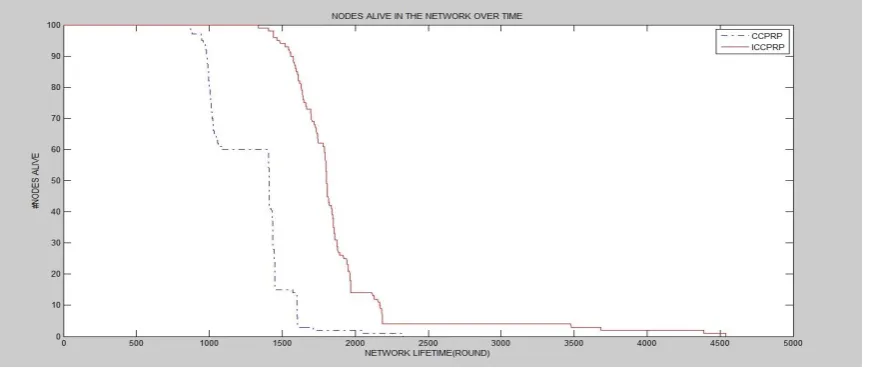
Both CCPRP and RPCC algorithms have been implemented in two level and three level heterogeneous network. Results show that RPCC perform better in both cases. In two level heterogeneous network ICCRP provides 68% more increase in service time with 100% sensing coverage ratio. In three level heterogeneous network ICCRP provides 21% more increase in service time with 100% sensing coverage ratio. Also the percentage of sensing coverage increases and connectivity is maintained till 5551th round in case of RPCC
as comparison to 2833th round in CCPRP.
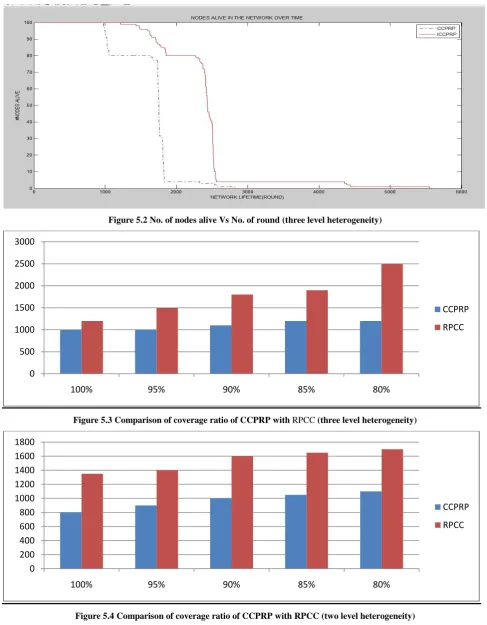
[image:5.595.83.518.540.725.2]In the following figures comparison is shown between CCPRP and RPCC algorithm. In both two level heterogeneity and three level heterogeneity it is evident that RPCC performs better than CCPRP. Coverage is calculated as number of nodes alive per round. Fig 5.3 and Fig 5.4 depicts no. of rounds upto which 100%,90%,80%,70% coverage is maintained. We can easily see RPCC perform better in both cases.
Figure 5.2 No. of nodes alive Vs No. of round (three level heterogeneity)
Figure 5.3 Comparison of coverage ratio of CCPRP with RPCC (three level heterogeneity)
Figure 5.4 Comparison of coverage ratio of CCPRP with RPCC (two level heterogeneity)
6.
CONCLUSION
In last we can conclude that Improved coverage and connectivity preserving routing protocol provides following
Advantages:
As Gateways are long distance communication nodes gateway must be towards sink. CHs must be
towards gateways as well as centre of cell. This will lessen the communication load on gateway and CHs.
3-level network heterogeneity is implemented which would definitely lessen communication load by using three different energy nodes.
0 500 1000 1500 2000 2500 3000
100% 95% 90% 85% 80%
CCPRP
RPCC
0 200 400 600 800 1000 1200 1400 1600 1800
100% 95% 90% 85% 80%
CCPRP
[image:6.595.57.541.71.280.2] Nodes with redundant coverage will be put in sleep modes hence coverage is maintained and connectivity can be preserved for longer time. The CCPRP algorithm is implemented with both two level heterogeneity and three level heterogeneity and results are compared with RPCC.In two level heterogeneity. RPCC provides 68% more increase in service time with 100%sensing coverage ratio. In three level heterogeneity RPCC provides 21% more increase in service time with 100%sensing coverage ratio. Also the percentage of sensing coverage increases and connectivity is maintained till 5551th round in case of ICCPRP as comparison to 2833th round in CCPRP. Hence in terms of a routing protocol that take into account coverage and connectivity RPCC performs better in both two level and three level heterogeneity case. In future the Routing protocol for coverage and connectivity(RPCC) can be adopted without knowing the exact location of the sensor nodes
7.
REFERENCES
[1] Amitabha ghosh and Sajal k. Das, Department of Computer Science and Engineering, University of Texas at Arlington, “Coverage and Connectivity Issues in Wireless Sensor Networks”, Mobile, Wireless, and Sensor Networks: Technology, Applications, 2006. [2] Habib M. Ammari and Raymond Mulligan, Wireless
Sensor and Mobile Ad-hoc Networks (WiSeMAN) Research Lab Department of Computer Science, Hofstra University, “Coverage in Wireless Sensor Networks: A Survey”, Network Protocols and Algorithms, ISSN 1943-3581, 2010, Vol. 2.
[3] Xin Liu, Department of Computer Science University of California, “Coverage with Connectivity in Wireless Sensor Networks”, NSF.
[4] Nurcan Tezcan, Wenye Wang, Department of Electrical and Computer Engineering North Carolina State University, “Effective Coverage and Connectivity Preserving in Wireless Sensor Networks”.
[5] Xiaorui Wang, Guoliang Xing, Yuanfang Zhang, Chenyang Lu, Robert Pless, christopher Gill, Department of Computer Science and Engineering, Washington University in St. Louis St. Louis, MO 63130-4899, “Integrated Coverage and Connectivity configuration in Wireless Sensor Networks” , Proceedings of the First ACM Conference on Embedded Networked Sensor Systems (SenSys'03).
[6] W. B. Heinzelman, et al., "An Application-Specific Protocol Architecture for Wireless Microsensor Networks," IEEE Transactions on Wireless Communications, vol. 1, pp. 660-670, 2002 .
[7] Georgios Smaragdakis, et al., "SEP: A Stable Election Protocol for Clustered Heterogenous Wireless Sensor Networks," in Proceedings of the 2nd International Workshop on Sensor and Actor Network Protocols and Applications, Boston, Massachusetts, 2004, pp. 121-129. [8] Dilip Kumar, et al., "EEHC: Energy Efficient
Heterogenous Clustered Scheme for wireless Sensor Networks," Computer Communications, vol. 32, 2009. [9] T. C. A. a. R. B. P. Dilip Kumar, "EECDA: Energy
Efficient Clustering and Data Aggregation Protocol for Heterogeneous Wireless Sensor Networks," International
Journal of computers, communications and control, vol. VI, pp. 113-124, 2011.
[10] Norah Tuah,Mohamod Ismail and Ahmad Razani Haron, “Energy consumption and lifetime analysis for Heterogenous Wireless sensor network “,IEEE 2013 Tencon –Spring.
[11] S. Meguerdichian, F. Koushanfar, M. Potkonjak, M.B. Srivastava, Coverage problem in wireless ad-hoc sensor networks, in: Proc. Of INFOCOM 2001.
[12] M. Cardei, J. Wu, Coverage in wireless sensor networks, in: M. Ilyas, L Magboub (Eds.), Handbook of Sensor Networks, CRC Press, 2004.
[13] Jamal N. Al-Karaki Ahmed E. Kamal, "Routing Techniques in Wireless Sensor Networks" ,IEEE Wireless Conununications,vol II,no .6,pp.6-28,2004. [14] H. Zhang and J. C. Hou, "Maintaining Sensing Coverage
and Connectivity in Large Sensor Networks," Journal onWireless Ad Hoc and Sensor Networks, vol. 1, pp. 89-123,2005.
[15] Ji Li , Lachlan L.H. Andrew, Chuan Heng Foh, Moshe Zukerman and Hsiao-Hwa Chen, Connectivity, Coverage and Placement in Wireless SensorNetworks ,Sensors 2009, 9,7664-7693.
[16] Chi-Fu Huang and Yu-Chee Tseng, The Coverage Problem in a Wireless Sensor Network, ACM MobiCom03,Sep. 2003,pp. 115-121.
[17] S. Kumar, T.-H. Lai, A. Arora, Barrier coverage with wireless sensors,in: Proceedings of the ACM/IEEE International Conference on Mobile Computing and Networking (MOBICOM) 2005, 2005, pp. 284-298. [18] B. Wang, W. Wang, V. Srinivasan, K. Chaing Chua,
Information coverage for wireless sensor networks, Cormnunications Letters, IEEE 9 (11) (2005) 967-969. [19] F. Ye, G. Zhong, S. Lu, L. Zhang, Energy efficient
robust sensing coverage in large sensor networks, UCLA Technical Report, 2002.
[20] T. Yan, T. He, John A. Stankovic, Differentiated SW'veillance for Sensor Networks, in: SenSys'03, Los Angeles, CA, USA, November 2003, pp. 5-7.
[21] M. Cardei, D. Du, Improving wireless sensor network lifetime through power aware organization, ACM Wireless Networks 11 (3) (2005) 333-340, May. [22] S. Slijepcevic, M. Potkonjak, Power efficient
optimization of wireless sensor networks, in: IEEE International Conference on Cormnunications, 2001. [23] S.-F. Hwang, Y.-y'Su,Y.-Y.Lin,C.-RDow,A
cluster-based coverage preserved node scheduling scheme in wireless sensor networks, in: IEEE The 3'd Annual International Conference on Mobile and Ubiquitous Systems, 2005, pp.I-7.
[24] K. Bae, H. Yoo n , Auton o m o us clustering scheme for wireless sensor networks using coverage estimation based self-proning, IEICE Trans. Commun . E88-8 (3)(2005) 973-980.
[26] Said B. Alla , Abdellah Ezzati ,” Coverage and connectivity preserving routing protocol for heterogeneous wireless sensor networks “,NGNS, (2012),ISSN : 2327-6533.
[27] S.Thiripura Sundari, P.Maheswara Venkatesh, Dr.A.Sivanantharaja ,” A Novel Protocol for Energy Efficient Clustering for Heterogeneous Wireless Sensor Networks “ , International Journal of Scientific & Engineering Research, Volume 4, Issue 8, August-2013 132 ISSN 2229-5518.
[28] Abdelkrim Haqiq, Driss Bouzidi, and Amine Berqia ,” Next Generation Networks and Services”, Vol.9 No.3&4 March1,2014.http://www.rintonpress.comjournals/jmm/ abstracts Jmm9-34.html
[29] V.K. Pandey and Dr. G.K. Upadhyay, “Impact of Wireless Communications Sensor Based Secure Networks “ , New York Science Journal 2012;5(11). [30] Norah Tuah, Mahamod Ismail and Kasmiran Jumari,”An
Energy-Efficient Node-Clustering Algorithm in Heterogeneous Wireless Sensor Networks: A Survey”, Journal of Applied Sciences, 12: 1332-1344
![Fig 1.Heterogeneous wireless sensor network architecture.[4]](https://thumb-us.123doks.com/thumbv2/123dok_us/8025090.767174/2.595.106.524.72.296/fig-heterogeneous-wireless-sensor-network-architecture.webp)